
Chapter 12. Microfluidics and Electrokinetic Flow Effects
12.1. Introduction
Microfluidics, as described here, refers to a fluidic regime (characterized by geometric length scales usually between 100 nm and 100 μm) in which the dominant transport physics change as compared to macroscopic fluid mechanics, due either to changes in Reynolds number, the relative importance of surface effects, or relative changes in the importance or character of different mixing and reaction processes. The tools used currently to understand microfluidic systems have historically been used to study flow in capillaries, both natural (in our circulatory system) and artificial (most commonly in glass capillaries), as well as flow through porous media such as soil. While the fluid mechanics tools have retained a similar structure, the applications have evolved, becoming more wide-ranging and more interesting with the development and ubiquity of microfabrication techniques.
Modern microfluidic systems are typically fabricated from glass, silicon, or a variety of ceramics and polymers. Initial systems were first developed in silicon and silica, owing to the prevalence of silicon micromachining expertise and the long history of using glass capillaries. More recently, a variety of polymeric substrates, including poly(dimethylsiloxane), polycarbonate, and poly(methylmethacrylate), have become more and more important due to their relatively low cost or their unique and useful properties.
Most microfluidic devices have been motivated by the desire to optimize fluidic handling for chemical, biological, and medical applications. Optimization can be achieved via massive parallelization or simply because the different fluidic regimes (e.g., surface-tension-dominated, electrokinetic) afford new techniques for manipulating and controlling fluids. Applications include protein crystallization as well as protein and DNA separation and identification, for which pictures of example devices are shown in Figure 12.1. Because of our interests in chemical/biological/medical applications, we will focus on primarily liquid-phase applications in this chapter.
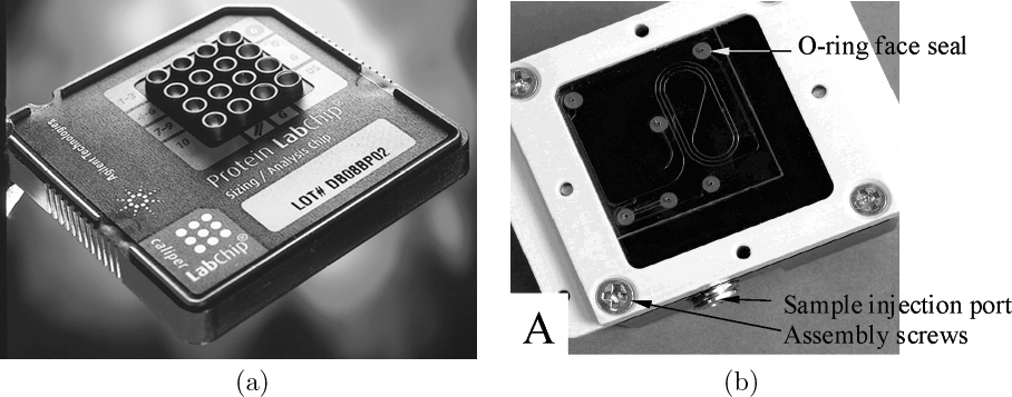
Fig. 12.1 Two examples of microfluidic chips. (a) Protein-sizing chip for use on Agilent 2100 Bioanalyzer. The 16 fluid reservoirs in the plastic caddy mate with the glass chip underneath. The microfluidic chip itself occupies just the area under the reservoirs. From A. Kopf-Sill Lab Chip, Vol. 2, pp. 42N–47N, 2002. Reproduced by permission of The Royal Society of Chemistry; (b) The microfluidic chip and fluidic compression manifold of the Sandia National Labs μChemLabTM microfluidic bioanalysis device. Reprinted with permission from R.F. Renzi et al., Analytical Chemistry, Vol. 77, pp. 435–441, 2005. Copyright 2005, American Chemical Society.
12.2. Physics of Microscale Fluid Mechanics
Dimensional analysis (Chapter 4) shows us that the character of flow through a given geometry depends only on the Reynolds number and not on the length scale per se. Similarly, scalar transport depends only on the Péclet number (defined using thermal diffusivity for heat-transfer problems or mass diffusivity for masstransfer problems). Why, then, discuss microfluidics separately from Stokes flow? The answer is that, despite the fact that many of the distinguishing aspects of microfluidic flows follow directly from their laminar, low-Re character, many others do not. Key differences in the relevant physics of microscale fluid transport include:
• Flows are typically laminar and have a low Reynolds number.
• Both pressure and electric fields are used to actuate flow, so the transport equations must be modified to include electroosmotic flow and electrophoresis of molecules or particles.
• Boundary conditions are often more difficult to define, since slip velocities need be included, depending on the length scale, and these slip velocities are often not well known or understood.
• If multiple phases exist, surface tension can dominate over pressure forces.
After a discussion specific to dispersion in pressure-driven flow in microscale tubes, this chapter will focus primarily on electrokinetic phenomena.
12.3. Pressure-Driven Flow Through Microscale Tubes
Recall the flow inside a circular pipe induced by a pressure gradient (Chapter 3). For a given pressure gradient and fluid, the character of the flow changes from laminar to transitional to turbulent as the diameter of the pipe is increased. Microfluidic channels have extraordinarily small diameters and therefore flow in microchannels typically occurs at low Re.
Example 12.1—Calculation of Reynolds Numbers
Calculate the Reynolds number Re for the following. Assume that the fluid has properties of water: density ρ = 1,000 kg/m3, viscosity μ = 10–3 kg/m s, and kinematic viscosity ν = 10–6 m2/s.
• Flow of drugs injected using thumb pressure (about 5 atm) on a 5-ml syringe through a ![]() -inch long, 27-gauge (internal diameter d approximately 300 μm) needle.
-inch long, 27-gauge (internal diameter d approximately 300 μm) needle.
• Flow of cell culture media at a mean velocity of 10 μm/s through a d = 20-μm diameter tube machined in a glass microchip, used to culture cells in what is called “continuous perfusion cell culture.”
• Flow of water at a mean velocity of 80 μm/s through d = 50-nm diameter tubes machined in silicon, used to sort and measure individual DNA molecules.
Solution
Syringe: Because of the high pressure drop, we anticipate that the flow is probably turbulent, in which case we can use Eqns. (3.33) for the pressure drop and (3.40) for the friction factor in a smooth tube:

Elimination of the friction factor and rearrangement gives the mean velocity:

thus verifying the assumption of turbulent flow.
DNA measurement:
12.4. Mixing, Transport, and Dispersion
Mixing is critical for countless chemical problems. Often, complete mixing is required to achieve a chemical reaction. In other cases, such as chemical separations, it is critical to minimize the extent to which different sections of fluid mix. Because microfluidic systems are used in both these situations, and because geometries of practical interest involve known solutions of the laminar Navier-Stokes equations, microfluidic systems serve as excellent model systems for discussing mixing and dispersion.
Taylor dispersion in a capillary tube. Consider the flow of two miscible liquids (for example, clear water and water with food dye mixed in). Specifically, consider a band of water with width w containing a species at concentration c0 amidst a flow of clear water (c = 0). As will be seen later, this flow is relevant to a number of chemical separations.
First we consider one-dimensional diffusion alone with no flow, and consider the radially averaged concentration ![]() . The equation governing the diffusion of the band is:
. The equation governing the diffusion of the band is:
And it can be shown that, for pure diffusion, the width of the concentration profile (which, for long times, is Gaussian in shape) grows as w α ![]() . Thus, as time proceeds, the width of the band increases proportional to the square root of time.
. Thus, as time proceeds, the width of the band increases proportional to the square root of time.
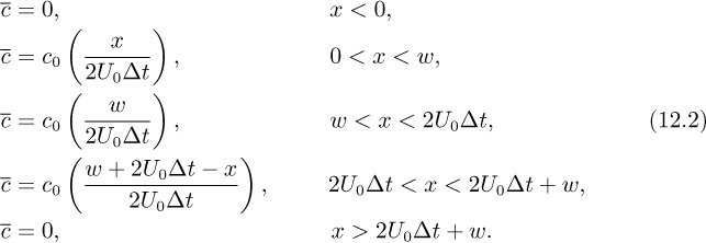
Consider now the opposite case. Ignoring diffusion and for the moment considering only convection, the parabolic velocity distribution distorts the interface between the two zones, as in Fig. 12.2.1 Given a parabolic velocity distribution with mean velocity U0 in a circular pipe, first note that the centerline velocity is 2U0; thus, a key quantity w/2U0 is the time taken for the liquid at the center to traverse a distance equal to the initial width w. It can be shown that for Δt>w/2U0, the radially averaged concentration c takes on a trapezoidal shape:
1 A short animation is available at http://www.fiu.edu/~thorned/LB/html/ani03poisseuille.html (yes, the website has the spelling “poisseuille”).
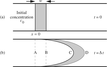
Fig. 12.2 Taylor dispersion caused by parabolic pipe flow: (a) initially; (b) at a later time Δt. See text for explanation.
From Eqns. (12.2) it is clear that, for this diffusionless flow, the maximum concentration c0 has been attenuated as the species are spread out by the flow; furthermore, the maximum height of the average concentration profile (c0w/2U0Δt) decreases linearly with time and the width of the profile increases linearly with time. The five segments of Eqn. (12.2) correspond to regions to the left of A, between A and B, between B and C, between C and D, and to the right of D.
Unsurprisingly, the two models (first, diffusion only; second, convection only) discussed above do not satisfactorily describe the observed sample band growth, since both omit a key aspect of the transport. Experimentally, it is observed that the growth of sample band width convected by parabolic pipe flow profiles increase proportional to the square root of time, but with a coefficient of proportionality larger than D1/2:

Here, the species diffusion Péclet number is defined as Pe = U0a/D, where a is the radius of the pipe. The Péclet number is analogous to the Reynolds number; whereas the Reynolds number expresses the ratio of advective fluxes of momentum to diffusive fluxes of momentum, the Péclet number expresses the ratio of advective fluxes of species concentration to the diffusive fluxes of species concentration.
As Pe becomes small (diffusion dominates), Eqn. (12.3) becomes equal to Eqn. (12.1). As Pe becomes large (diffusion can be neglected), the term 1 + Pe2/48 becomes large, and diffusion is rapid. Note that the applicability of Eqn. (12.3) does not extend to Pe = ∞, so the result in Eqn. (12.2) cannot be recovered by simple substitution in Eqn. (12.3). Since we expect to apply Eqn. (12.3) to microscale flows, Re is small. Note, however, that we often deal with samples with very large Schmidt numbers (Sc = Pe/Re) since their diffusivities are very low. Thus, Pe values as high as 1,000 are common, even in microfluidic applications.
12.5. Species, Energy, and Charge Transport
Before addressing the double layer per se, we must expand the transport equations from Chapter 5 to include chemical species, thermal energy, and charge. The discussion is by necessity brief, and much of the derivation is left for the reader.
Constitutive relations. Recall from Chapter 5 that the heat flux q defines the rate at which thermal energy is conducted due to temperature gradients and that Fourier’s law states:
This constitutive relation is the necessary link between the temperature field and the governing transport equation that expresses conservation of thermal energy fluxes, just as Newton’s law of viscosity is the necessary link between the velocity field and the governing transport equation for conservation of fluid momentum. Fick’s law of diffusion:
similarly relates the species diffusive mass flux Ji to the gradient of the species mass density ρi.
While the constitutive relations that govern diffusion for species and temperature are quite similar, we must consider different effects when we treat charged species in an electric field. If a gradient in the electrostatic potential is present, a force is exerted on a charged molecule. The electric field E is defined as the negative gradient of the electrostatic potential:
and the force exerted on a molecule is given by
where q is the charge number (the electrical charge normalized by the elementary charge, 1.602 × 10⁻¹⁹ coulombs) and e is the elementary charge (1.602 × 10⁻¹⁹ C). An electric field is thus seen to cause a force that is proportional to that field. The motion of ions is retarded, though, by collisions with the surrounding molecules. In the steady state, the ion motion (termed electrophoresis) takes on a velocity given by:
and the molar charge flux is
where c is the species concentration. The electrophoretic mobility μep is typically determined experimentally; values of μep for some small ions are given in Table 12.1.
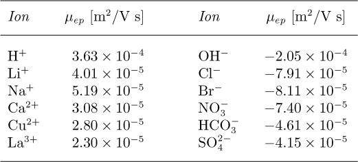
† Values calculated from G. Atkinson, 1972: “Electrochemical information,” in American Institute of Physics Handbook, 3rd ed., (ed. D.E. Gray), pp. 5-249–5-263, McGraw-Hill, New York.
Transport equations. In Chapter 5, the transport equations for momentum (i.e., the Navier-Stokes equations) were derived. The transport equations for temperature, species, and charge are similar. We will treat mass and thermal energy as conserved scalars, i.e., we will assume that they are transported by the fluid flow but are neither created nor destroyed. To make this approximation, our assumptions include: (a) that no chemical reaction occurs, and (b) that the heat generated by viscous dissipation can be assumed small. With these assumptions, and using the convective derivative D/Dt we can write a transport equation for a species concentration:
and temperature:
Note that Eqns. (12.9) and (12.10) are similar to the Navier-Stokes equations (Eqn. (5.68)) except that: (a) there is no pressure or gravity forcing term involved,
(b) species molar diffusivity D or thermal diffusivity α plays the same role as the kinematic viscosity μ/ρ, and (c) the equations are linear (the nonlinearity in the Navier-Stokes equations stems from the nonlinear convective term). Also note that the species and temperature transport equations, as written, do not couple back to the Navier-Stokes equations—that is, the fluid flow affects species and temperature transport but the species and temperature transport does not affect the flow. The same cannot be said for electrical charge, for which the laws of electrodynamics must be coupled to the flow equations.
If we assume that magnetic fields may be ignored (i.e., externally applied magnetic fields are small, current-induced magnetic fields are small, and the electric field is quasi-steady), then the system can be assumed electrostatic and the electrical potential φ is related to the local charge density via Poisson’s equation:
where ρe is the local net charge density, and ε is the electrical permittivity of the liquid. The electrical permittivity of free space, ε0, is equal to 8.85 × 10⁻¹² C/V m; the permittivity of various materials are typically described through their dielectric constant, ε/ε0. The dielectric constant of water at room temperature is approximately 80.
Just as a gravitational body force term ρg must be included in the Navier-Stokes equations when gravity plays a role (e.g., Eqn. (5.68)), so must the Lorentz body force term be included when there is a net charge density and an electric field. This term can be written as:
where fLorentz is the force (per unit volume) caused by the electrostatic force felt by the charge density ρe in the electric field. With this force, the Navier-Stokes equations relevant for microfluidic applications become:
Note that gravity has been ignored and incompressibility has been assumed. The effect of the Lorentz force will be of immediate impact when we discuss the electrical double layer and the microscopic derivation of the electroosmotic flow velocity.

12.6. The Electrical Double Layer and Electrokinetic Phenomena
If one drinks water from a glass, there is hardly any reason to think that electric fields play a prominent role in the motion as the water pours out into one’s mouth. However, we can infer from some simple experiments that electric fields do play a significant role in fluid transport at small scales. For example, if a pressure gradient of 5 atm is applied to water to induce Poiseuille flow through a glass capillary of, say, 100 μm diameter, a voltage difference of approximately 1 volt can be measured between the two ends of the capillary. Similarly, if the pressure is removed and a voltage gradient (say 10 kV/m) is applied across the same capillary, the water inside will be observed to move uniformly at approximately 1 mm/s. These phenomena stem from an electrochemical phenomenon known as the electrical double layer, discussed in this section.
Electroosmosis. Before discussing the detailed root cause of the electrical double layer, we will begin by describing its most obvious effect—electroosmotic flow. Experiments show that if an extrinsic electric field E is applied across a tube containing an electrolyte solution, a uniform flow will result, with a velocity given by:
Here, ζ is called the zeta potential, and μeo ≡εζ/μ is termed the electroosmotic mobility. Both of these values are functions of both the wall material and the nature of the liquid. Unlike Poiseuille flow through a tube, the velocity of this flow is not a function of the size of the tube, within certain limits (roughly speaking, for tube diameters above 100 nm or so). Figure 12.3 shows the velocity distribution for electroosmotic flow as compared to pressure-driven flow.
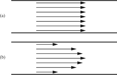
Fig. 12.3 (a) Electroosmotic flow in a tube can be approximated as uniform throughout; (b) laminar pressure-driven flow in a tube takes on the well-known parabolic form.
Example 12.2—Relative Magnitudes of Electroosmotic and Pressure-Driven Flows
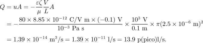
Consider a circular tube of diameter d = 5 μm (r = 2.5 μm) and length L = 10 cm filled with an aqueous solution. If ζ = –100 mV, calculate the pressure required to give the same total flow that would be generated by the application of 1 kV.
Solution
Electroosmotic flow:
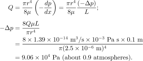
Pressure-driven flow:
Detailed structure of the electrical double layer. The simple preceding discussion is an accurate description of the majority of the flow field and predicts velocities and flow rates quite well; however, it is certainly dissatisfying from the standpoint of our intuition regarding the boundary conditions that apply to fluid flow. By describing electroosmotic flow as uniform, we are implying that the velocity at the wall is equal to the bulk velocity (i.e., full slip and a completely inviscid interface)! In the following paragraphs we will show that indeed the noslip condition applies, but the region in which the flow is retarded is remarkably thin and, for the purposes of mass flow rate, can be ignored.
From a fluid mechanics point of view, we consider the wall to be simply the location of the no-slip boundary condition; chemically, however, things are much less simple. The surface chemical groups on the wall undergo reactions with the liquid and achieve an equilibrium chemical state. The surface charge at the wall is in general nonzero since these reactions typically involve adsorption of charged ions or creation of charged groups by addition or removal of protons from the surface material. The details of the surface chemistry are beyond the scope of this discussion; however, in general we can assume that the surface has a nonzero charge. Further, we can assume that the aqueous solution has some concentration of electrolytes (even pure water has 10–7 M H3O+ and 10 –7 M OH –).
When an electrolyte solution comes into contact with a charged surface, the charged surface locally changes the ion distribution (which would otherwise be uniform). Ions with an opposite charge to the surface (termed counterions) are attracted to the surface, while ions with similar charge (termed coions) are repelled. An equilibrium is achieved between: (a) electrostatic attraction/repulsion and (b) Brownian (thermal) motion, which tends to distribute ions randomly in an exponential (Boltzmann) distribution, as in Fig. 12.4.

Fig. 12.4 Structure of the electrical double layer. The situation shown is for a negatively charged surface (O–), with a negative zeta potential. The monolayer with the occasional K+ion is the Stern layer. Note the preponderance of positive ions in the double layer.
The Boltzmann distribution can be derived from equilibrium arguments that say the likelihood of a system being in a state with molar potential energy E is proportional to e–E/RT. The potential energy of a mole of charge held at a potential φ is E = qF φ, where q is the ion charge (for example, q+ = 1 for Na+, q– = –1 for Cl–, q+ = 2 for Mg2+, etc.) and F is the Faraday constant, 9.65 × 10⁴ C/mol. If the molar concentration of ions in the electrolyte solution far from the wall (where the potential is zero) is c∞, the concentration of ions at a location with a potential φ conforms to Boltzmann’s equation:
As the potential becomes more positive, the concentration of positive ions will decrease and that of negative ions will increase.
If the counterions and coions have charges with the same magnitude (e.g., +1 and –1 or +2 and –2), the net charge density (see Problem 12.9) is given by:

where z = |q| is the valence of the ions (the magnitude of the charge normalized by the electron charge, for example, 1 for Na+ and Cl– and 2 for Mg2+ and ![]() ), c+ and c– are the concentrations of positive and negative ions, respectively, and φ is the local potential. The combination of the Poisson equation (Eqn. (12.11)) with the Boltzmann charge distribution of Eqn. (12.16) gives a relation termed the nonlinear Poisson-Boltzmann equation, which in a one-dimensional system (such as an infinite flat plate) is:
), c+ and c– are the concentrations of positive and negative ions, respectively, and φ is the local potential. The combination of the Poisson equation (Eqn. (12.11)) with the Boltzmann charge distribution of Eqn. (12.16) gives a relation termed the nonlinear Poisson-Boltzmann equation, which in a one-dimensional system (such as an infinite flat plate) is:
where x is the distance from the edge of the Stern layer.
Recall that the Poisson equation relates the Laplacian of the potential field to the charge density—here the charge density is directly related to the exponential distribution of both counter- and coions. Again, we have assumed a symmetric electrolyte, that is, that the charge of the positive ions is equal to the charge of the negative ions. Generalizing to multiply-valent ions is straightforward (but algebraically complex) and adds little to this discussion.
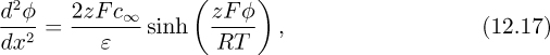
Equation (12.17) can be simplified considerably by defining the Debye length, followed by a suitable normalization of the potential. The Debye length θD is defined as ![]() this length is approximately equal to the thickness of the double layer and will later be shown to be the characteristic length of the exponential decay of the potential in certain situations. We can also normalize φ by RT/zF (φ* = φzF/RT);RT/zF is the potential at which a coion of valence z has potential energy equal to RT. With these definitions, Eqn. (12.17) can be rearranged to give:
this length is approximately equal to the thickness of the double layer and will later be shown to be the characteristic length of the exponential decay of the potential in certain situations. We can also normalize φ by RT/zF (φ* = φzF/RT);RT/zF is the potential at which a coion of valence z has potential energy equal to RT. With these definitions, Eqn. (12.17) can be rearranged to give:

If φ* ≪ 1 (the so-called Debye-Huckel limit), the one-dimensional nonlinear Poisson-Boltzmann equation can be simplified (by using the approximation sinh x ![]() x) to give (the asterisks can be removed from both sides):
x) to give (the asterisks can be removed from both sides):
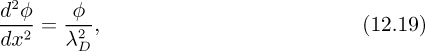
which, for a flat plate in an infinite reservoir, leads to exponential solutions:
The zeta potential, ζ, is the potential at the wall (x = 0), and the Debye length is the 1/e decay distance of the potential as the distance from the wall increases. For univalent electrolytes, θD is approximately 10 nm at 1 mM concentration.
We now consider electroosmosis in detail. Modeling the flow in the double layer as unidirectional and one-dimensional, and combining the Navier-Stokes equations (with the Lorentz source term, Eqn. (12.13)) with the Poisson equation (Eqn. (12.11)), a relation can be derived (see Problem 12.10) between the flow and the potential in the double layer:
This relation has separated the potential field into two components: (1) the intrinsic potential due to the surface charge, denoted by φ, and (2) the extrinsic potential applied to drive the electroosmotic flow, denoted by the externally applied electrostatic field Ey.
Equation (12.21) may be integrated. For a flat wall in an infinite reservoir of fluid, this is straightforward analytically; requiring that the velocity is bounded at x = ∞ and zero at the wall, we can show that
which is valid for all x. From Eqn. (12.22) we note that, for a flat surface, the fluid velocity and the intrinsic potential in the double layer are similar, i.e., they have the same functional form. Thus the velocity and potential can be graphed simultaneously, as done in Fig. 12.5.
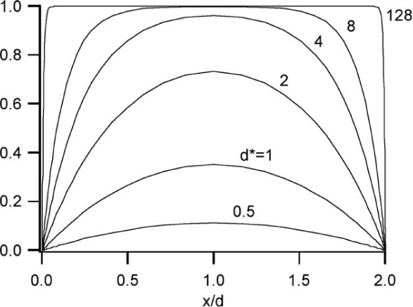
Fig. 12.5 Electroosmotic flow and potential distributions between two infinite parallel plates separated by a distance 2d. Spatial profiles of nondimensionalized velocity u* = u(εζE/μ)–1 are shown as a function of d* = d/λD, the ratio of the half width to the Debye length. Calculations are shown in the Debye-Huckel limit (i.e., solutions to Eqn. (12.19)).
One particularly illustrative solution of Eqn. (12.19) (or, more generally, Eqn. (12.18)) is the solution between two infinite parallel plates. This solution (Fig. 12.5) shows the impact of wall spacing on the character of the potential distribution and, as we will see in the following paragraph, electroosmotic flow. For large wall spacings (as compared to the double layer thickness, which can be characterized using the Debye length), the potential is uniform throughout most of the fluid, decaying rapidly to the zeta potential in thin layers near the walls. Such a profile is typified by wall spacings roughly 100 times the double layer thickness, or > 1 μm at 1 mM concentration. This is the regime described by the introductory discussion. When the wall spacing is no longer much greater than the double layer, the potential can no longer be described as largely uniform, and the resulting average electroosmotic velocity is no longer given by u = –εζE/μ.
Similitude between the velocity field and the extrinsic electric field. Recall from Chapter 7 that, absent electrokinetic effects, vorticity is generated at fluid-wall interfaces and propagates from the interfaces into the flow. The vorticity transport equation, though, has no source term, i.e., vorticity is not generated within the flow field. In Chapter 7 it was noted that, far from solid boundaries, the vorticity is often small and can be neglected. One of the more interesting results of electroosmotic flow is that the flow is irrotational outside the electrical double layer, and thus the flow field is given by a solution of Laplace’s equation. In fact, it can be shown that if ζ is constant, double layers are thin compared to the geometry or the radius of curvature of any geometric features, and if electrokinetic forces are the only flow effects (i.e., no pressure gradient exists) the simple relation in Eqn. (12.14) applies to the entire flow field (except the double layer) regardless of the complexity of the geometry.
Thus, the electrical potential and the velocity potential differ only by the multiplier εζ/μ. The formal proof of this requires substantial vector operations, and will not be covered here. Equation (12.14) thus shows that, outside the double layer, the extrinsic electric field and the velocity are similar (i.e., proportional to each other). This similitude and the ability of Laplace’s equation to produce the flow solution has several results. First of all, Laplace’s equation is much more easily solved than the Navier-Stokes equations, both analytically (for which the Navier-Stokes equations typically have no solution) and numerically (for which the Navier-Stokes equations require more computing power). Second, the uniform flow allows fluid samples to be moved throughout a microchannel without dispersing the sample.
Example 12.3—Electroosmotic Flow Around a Particle
Assume a spherical particle of diameter a ≫ λD is suspended and held stationary inside a microchannel with diameter d ≫ a and that the particle and channel are made from the same material and have the same surface potential. An electric field E∞ is applied to the system. Calculate the flow solution (in terms of velocity potential φ) around this particle.
Solution
Recall from Eqns. (7.71)–(7.74) and Fig. 7.17 that potential flow around a sphere can be modeled as the superposition of a uniform stream (φ = Ur cos θ) with a doublet of strength s = –Ua3/2, for which φ = Ua3 cos θ/2 r2. This solution identically solves the electroosmotic flow around a particle, with U given by εζE∞/μ. Since d ≫ a, it is correct to model the electroosmotic flow as a uniform stream.
Example 12.4—Electroosmosis in a Microchannel (COMSOL)
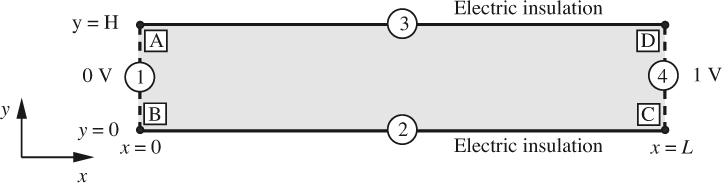
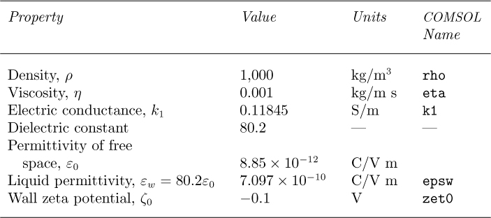
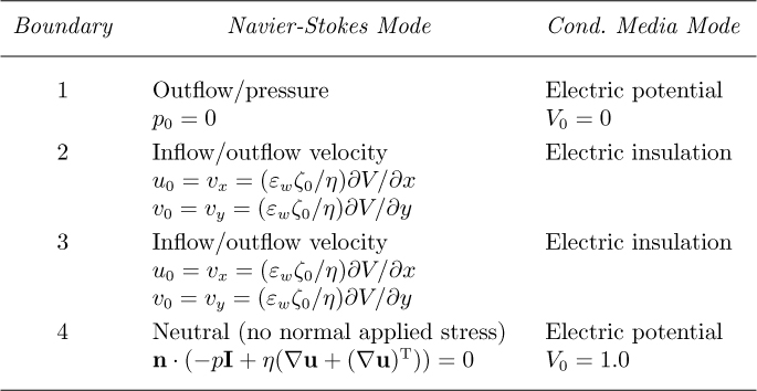
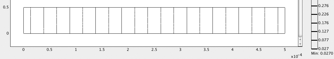
The microchannel ABCD in Fig. E12.4.1, with length L = 5 × 10⁻⁴ m and width H = 5 × 10⁻⁵ m, contains an electrically conducting liquid whose physical properties are given in Table E12.4.1, in which “S” denotes units of Siemens, also equivalent to ohm –1. Note also that a coulomb (C) equals an ampere-second (A s), and that the dielectric constant is also known as the relative permittivity. Electric potentials of zero and 1 V are applied at the left and right ends AB and CD, respectively, and we wish to find the resulting liquid velocities and electric potential distribution.
Solution
This problem falls into the multiphysics category, in that it involves both simultaneous motion of fluid and electric charge. In the Model Navigator, make sure the New tab is highlighted. Then, under Fluid Dynamics, select Incompressible Navier-Stokes, followed on the right-hand side by Multiphysics, and Add. Repeat the procedure for Electromagnetics, Conductive Media DC, Add, followed by OK, so the stage is all set in the graphical user interface for multiphysics—which you can check by pulling down the Multiphysics menu, which will display both modes:
1. Incompressible Navier-Stokes (ns).
2. Conductive Media DC (dc).
Later, when media properties and boundary conditions are being set, we can toggle between the two modes.
Now execute the following steps:
1. Draw the rectangle ABCD.
2. Under Options/Constants, store the values from Table 12.4.1 for rho, eta, k1, epsw, and zet0, followed by OK. As usual, you make the appropriate entries in the “Name” and “Expression” columns (the latter may contain arithmetic operators), and the “Value” column is automatically computed.
3. Under Physics/Subdomain Settings, for the two modes, indicate that rho and eta are the expressions for the density and dynamic viscosity, and that k1 is the conductivity. To switch from one mode to the other, use the Multiphysics pulldown menu.
4. Under Physics/Boundary Settings, for the two modes, set the boundary conditions given in Table E12.4.2, noting for example that Vx is the COMSOL designation for ∂V/∂x, the x-derivative of the electric potential. Thus, the entry for u0 will be (epsw*zet0/eta)*Vx. Cutting, pasting, and editing expressions will save time.
5. Initialize and refine the mesh twice, as in Fig. E12.4.2, noting the number of elements and degrees of freedom.

6. Under Solve/Solver Parameters, click on the Advanced tab, and change Scaling of variables from Automatic to None—an essential step for the following none-too-obvious reason. Namely, for accuracy in solving simultaneous equations, COMSOL tries to scale the dependent variables so that they are all of order 1. The scaling is accomplished by dividing each variable by a reference quantity. But in our present problem, because there is no applied potential difference in the y direction, there is no flow in that direction, so that υy = 0 and the scaling is impossible. If this precaution were not taken, the attempted solution would not converge.
7. Solve the problem.
Results and Discussion
1. Generate and print an arrow plot of the velocities, shown in Fig. E12.4.3. Note that in line with electroosmotic theory, the velocity is constant everywhere, and that the liquid, which has a negative zeta-potential ζ0 (and hence an excess of positive ions next to the walls), flows uniformly in the direction of decreasing electric potential—from right to left.
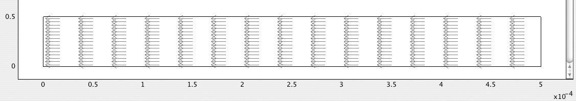
2. Generate and print a streamline plot—Fig. E12.4.4 shows the streamlines as parallel straight lines pointing in the negative x-direction. To obtain full control, begin with Plot Parameters/Streamline/Specify start point coordinates, and specify x: linspace(0,0,10) and y: linspace(0,5e-5,10), which will ensure ten streamlines, all starting along AB (x = 0) and then being equally spaced along AB (between y = 0 and y = 0.00005).
3. Generate a surface plot of the velocity distribution (not reproduced here) and note—by both observing the color bar at the right and also clicking on various points and looking at the lower left-hand corner—that the velocity is everywhere essentially uniform, with a value of 1.42 ×10 –4 m/s (in the negative x direction, as evidenced by the arrow plot).
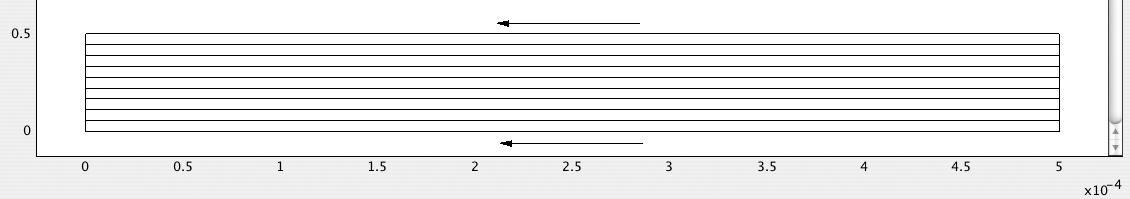
4. Generate and print a contour plot of the electric potential—Fig. E12.4.5 shows a series of equally spaced equipotentials, varying from 1 V at the right-hand boundary CD to zero at the left-hand boundary AB.
Example 12.5—Electroosmotic Switching in a Branched Microchannel (COMSOL)
This example investigates the possibility of using electroosmosis as a “switching” mechanism for controlling the flow of liquids in microchannels.
Modify Example 12.4 so that it now includes a “vertical” branch of width 5 × 10⁻⁵ m, extending in “height” as far as y = 2.5 × 10⁻⁴ m, as shown below. Investigate the streamlines and equipotentials for the two sets of applied voltages shown in Figs. E12.5.1 and E12.5.2. All physical properties are identical with those given in Example 12.4.
Solution
The solution is very similar to that of Example 12.4, and most of the basics will not be repeated. The easiest approach is to make of copy of the *.fl file from the previous example and modify it. The additional rectangular channel extending in the y direction is easily added to the existing rectangle of Example 12.4 by forming a composite object, unchecking Keep interior boundaries. To smooth the corners where the two rectangles join, observe the following steps:
1. Select the Fillet/Chamfer drawing tool (the bottom tool at the left of the screen) and highlight the Fillet option.
2. Under Vertex selection, click on the composite object icon, and note that eight vertices are listed.
3. Find the vertex that corresponds to the coordinates (2.25 × 10 –4,0.5 × 10 –4), enter a radius of 0.25 × 10 –4, and click OK.
4. Repeat for the vertex a little further to the right.
No changes are needed to the Physics/Subdomain settings. For boundary conditions, under the Physics/Boundary Settings, first enter the three electric potentials, –1, 0, and 1 V, shown in Fig. E12.5.1, and, for the Navier-Stokes boundaries, note that the right and upper channel entrances will be “neutral.” Otherwise, the boundary conditions are very similar to those of Example E12.4 shown in Table E12.4.2, namely, “electric insulation” for the conductive media mode and “inflow/outflow velocity” for the Navier-Stokes mode.
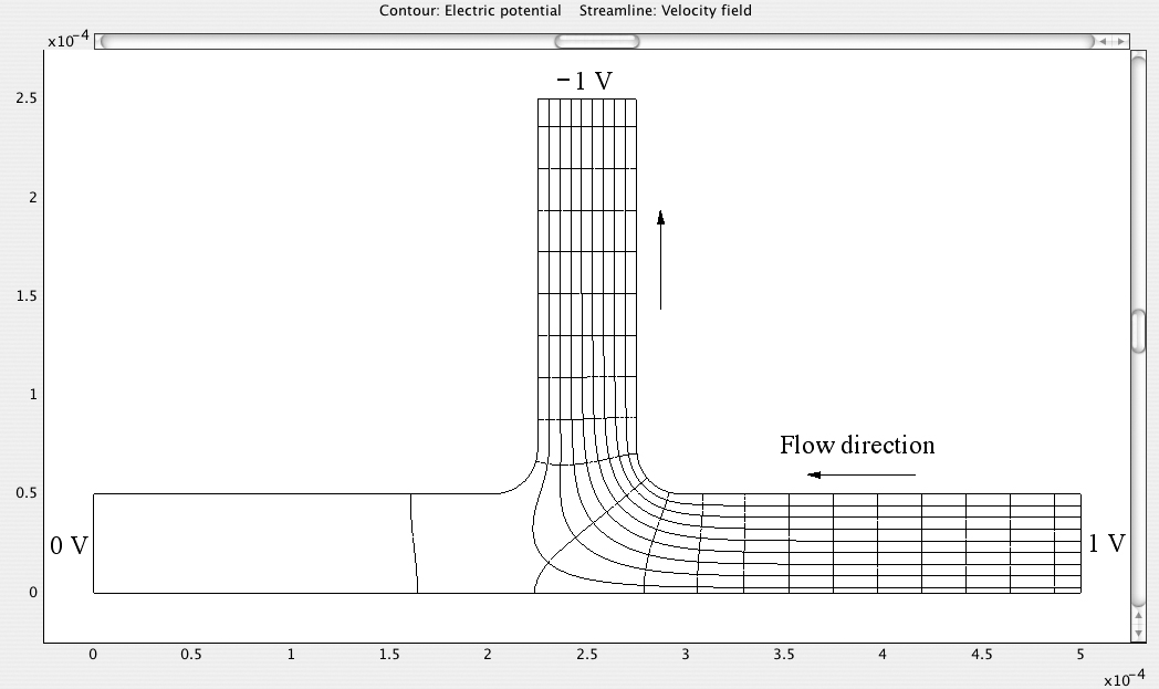
Fig. E12.5.1 Streamlines and equipotentials for applied potentials of 0, 1, and –1 V at the left, right, and upper ends of the branch, respectively.
Initialize the mesh (no refinement is needed) and solve the problem. Because there is now a flow in the y-direction, under Solve/Solver Parameters the scaling of variables can be left as Automatic under the Advanced tab.
Finally, display the results as a superposition of streamlines and equipotentials, as in Fig. E12.5.1. To accomplish this, under Postprocessing/Plot Parameters:
1. Under General, check both Contour and Streamline.
2. Under Contour/Predefined quantities, select Electric potential (dc). Repeat the process for the three electric potentials shown in Fig. E12.5.2.
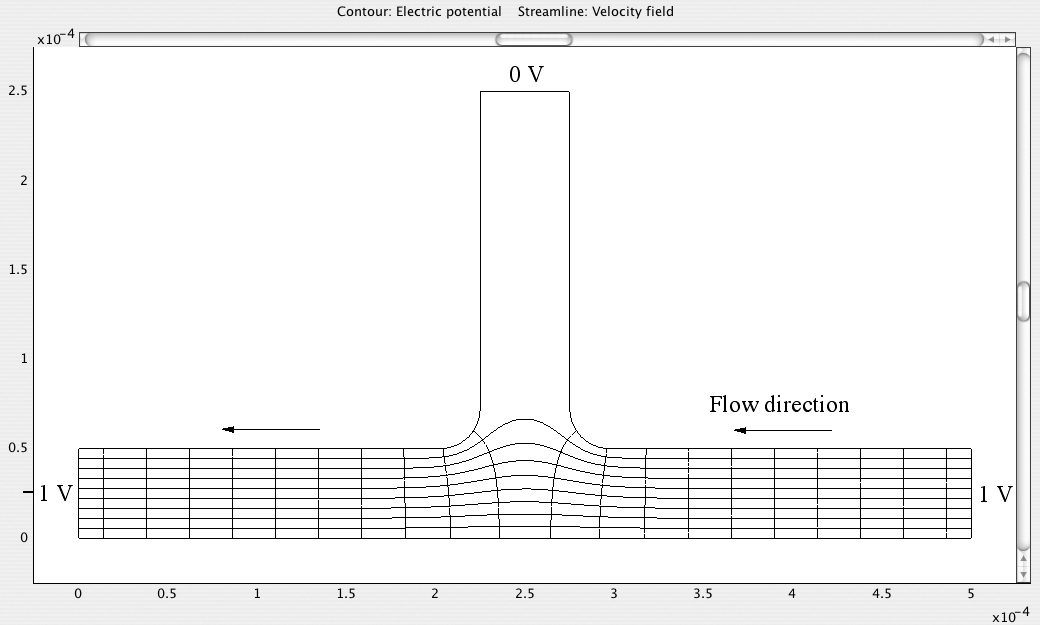
Fig. E12.5.2 Streamlines and equipotentials for applied potentials of –1, 1, and 0 V at the left, right, and upper ends of the branch, respectively.
3. We wish to ensure ten streamlines, all starting along the right-hand entrance (x = 5 × 10⁻⁴) equally spaced between y = 0 and y = 0.5 × 10 –4. Under Streamline/Specify start point coordinates, specify x: linspace(5e-4,5e-4,10) and y: linspace(0,5e-5,10).
Discussion of Results
From the two diagrams, it is very apparent that the direction of liquid flow can be controlled by suitable adjustment of the applied voltages. Observe that in both cases the entrance to the system that has no flow has an electric potential (of zero) that is midway between those of the entrances between which there is a flow. Note also that the streamlines are everywhere orthogonal to the electric equipotentials.
By a similar adjustment of electric potentials, liquid flows can be controlled in a much more complex arrangement of microchannels.
12.7. Measuring the Zeta Potential
Two major techniques exist to determine the zeta potential experimentally:
1. Measuring electroosmotic velocities.
2. Measuring the streaming potential.
Electroosmotic velocities. The measurement of electroosmotic velocities is the most straightforward and intuitive technique for measuring the zeta potential. Recall from Eqn. (12.14) that the electroosmotic velocity is proportional to the applied electric field. If the electroosmotic velocity is measured under a known applied electric field, the zeta potential may be calculated directly. Electroosmotic velocities can be measured by optically tracking uncharged fluorescent tracers, weighing a volume of electroosmotically driven fluid to determine the mass flow rate and therefore the average velocity, or by tracking changes in electrical current as fluids with different conductivity are moved through a channel.
Streaming potential. Streaming-potential techniques are a less obvious but effective experimental means for measuring the zeta potential. Consider pressure-driven flow through a capillary with radius a and zeta potential ζ. Assume that the double-layer thickness is small compared to a and that the Debye-Huckel approximation may be made. In this case, the charge density near the wall is given by:
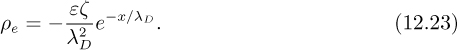
The Hagen-Poiseuille flow through this capillary will tend to displace this charge density and transport it along the capillary. This net charge transport (i.e., current) is given by the integral of the velocity/charge-density product:
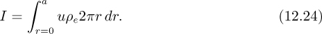
This current leads to a potential buildup at the downstream end of the capillary. At equilibrium, the current induced by the fluid flow is balanced by the current due to this potential. It can be shown (see Problem 12.15) that for a fluid with conductivity σ, the equilibrium potential difference is given by:
in which ΔV = Voutlet – Vinlet and Δp = poutlet – pinlet. Eqn. (12.25) is a rather remarkable result. The streaming potential, in the thin-double-layer, Debye-Huckel limit, is not a function of the geometry of the capillary, nor is it a function of the double layer thickness!
Example 12.6—Magnitude of Typical Streaming Potentials
Above, we asserted that streaming potential can be used to measure the zeta potential. Of interest is the magnitude of these streaming potentials. Consider a capillary subjected to a pressure difference of 5 atmospheres (this is easy to generate with a handheld syringe), inducing flow of an aqueous solution with a conductivity of 180 μS/cm. If the surface zeta potential is –20 mV, what will the measured streaming potential be? Will these voltages be easy to measure?
Solution
The Helmholtz-Smoluchowski equation gives:

in which the outlet (low pressure) will have the more positive voltage. Voltages on the order of 1 volt are quite easy to measure!
12.8. Electroviscosity
An additional consequence of the streaming potential described in the previous section is a phenomenon known as electroviscosity. When pressure is used to induce flow through small capillaries, the observed flow rate is at times below that value calculated using the Hagen-Poiseuille solution for flow in a circular tube. The reason for this is that the streaming potential generated by a pressure-driven flow induces a counterpropagating electroosmotic flow that tends to reduce the net flow rate. If one does not account for electrokinetic effects, this reduction in flow rate appears to result from an increase in viscosity in the fluid, hence the term electroviscosity; however, this phenomenon has nothing to do with changes in viscosity.
A detailed treatment of electroviscosity can involve quite detailed and extensive integration; however, we will consider electroviscosity in a simple manner only. In general, pressure applied to a circular pipe or capillary will induce a flow rate from the Hagen-Poiseuille solution:

Eqns. (12.14) and (12.25) can be combined to give the counterpropagating flow due to streaming potential-induced electroosmosis:

For low-conductivity solutions (e.g., deionized water) and small channels (< 1 μm), the counterpropagating flow can become significant. For electrolyte solutions at 0.1 mM or higher concentration and channels larger than 1 μm, electroviscosity can safely be neglected.
12.9. Particle and Macromolecule Motion in Microfluidic Channels
In this section we are concerned with the motion of particles and macromolecules in microfluidic channels. The particles of interest include:
• Solid microspheres, typically made from latex or silica, often used for a variety of biochemical assays.
• Insoluble colloids.
• Cells.
The macromolecules of interest are typically polymers, and include:
• Synthetic polymers (e.g., polyacrylamide, polyethylene glycol).
• Proteins (polymers of amino acids).
• Ribonucleic acids (e.g., DNA and RNA, polymers of ribonucleotides).
• Carbohydrates (polymers of sugars).
We will start by considering particles. The particles of interest in microscale flows typically have sizes ranging from 10 nm to 10 μm; if we assume typical velocities of 10–5 to 10–3 m/s, typical Reynolds numbers (in water) will range from 10–2 to 10–7. Thus, the flow around these particles is well within the low Reynolds number Stokes limit.
First, consider the Stokes drag on a particle. Recall the following from Chapter 4:
1. The flow regime (laminar vs. turbulent) is based on the particle Reynolds number Re = ρμd/μ, where d is the particle diameter.
2. The transition from laminar to turbulent occurs gradually, and only flows with Re < 1 are completely laminar.
3. The drag coefficient ![]() is used for correlating the drag with the Reynolds number.
is used for correlating the drag with the Reynolds number.
4. For Re < 1, CD = 24/Re and Stokes law gives FD = 3πμu∞D.
5. Particles settle when a body force such as gravity is applied. The terminal velocity is reached when the drag force equals the body force.
Example 12.7—Gravitational and Magnetic Settling of Assay Beads
Problem Statement (Part 1)
Numerous biochemical assays use solutions of magnetic beads. Typically, a solution of beads is flushed into a system where a chemical reaction takes place at the surface of the beads (perhaps chemical binding due to antibodies). Magnets are used to control whether beads flow freely or are held stationary, as in Fig. E12.5. Two characteristic settling times are important:
1. The gravitational settling time (i.e., how long can a solution of beads be stored before the beads fall to the bottom of the container?).
2. The magnetic trapping time (i.e., how quickly will a magnet pull the particles into a wall?).
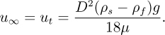
Given that Re < 1 for a microsphere, derive the terminal velocity for a microsphere. Estimate the settling time in hours for 1-μm diameter magnetic microspheres in water in a container of height L = 1 cm by calculating the time required for particles at the terminal velocity to travel 0.5 cm. Assume that the magnetic microspheres have a density of 4 g/ml.
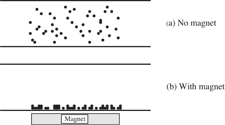
Fig. E12.5 Magnets can be used to control the movement of particles. This is typically used to facilitate flushing steps for chemical assays.
Solution
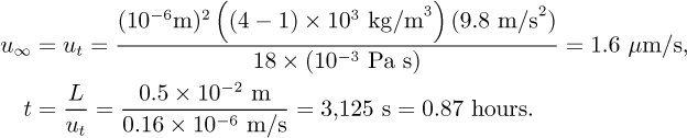
For Re < 1, FD = 3πμu∞D. Since the drag force must balance the gravitational body force (πD3/6)(ρs –ρf)g):
Then evaluate:
Problem Statement (Part 2)
Assume that a magnet is used to apply a magnetic force FM of approximately 1 pN to these microspheres, which is a typical value for polystyrene beads with ~15% ferrite and typical rare-earth magnets. How many seconds would it take for these microspheres to move from one end of a 20-μm diameter channel to the other? As before, use the terminal velocity to estimate the elapsed time.
Solution
Electrokinetic forces. Having discussed the impact of Stokes flow solutions on particle motion in a flow with body forces, let us now turn to particle migration with surface forces, namely electrokinetic forces. As was indicated earlier, voltage is often used in microfluidic systems to actuate ions, particles, or fluids. Electrophoresis is the term used to denote the motion of an electrically charged molecule or particle in response to an electric field.
The electrophoretic velocity of a particle can be predicted using arguments similar to those used to derive the electroosmotic velocity of flow past an immobile surface. Presuming the double layer is thin compared to the diameter of the particle, the one-dimensional relations derived earlier hold, and the electrophoretic velocity of the particle—relative to any other liquid motion—is again given by:
where ζp is the zeta potential of the particle surface. Note the absence of a minus sign in Eqn. (12.28)—in electrophoresis a negative particle (for example) is attracted to a positive electrode, while in electroosmosis the positive ions near a negative wall are attracted to a negative electrode. Eqn. (12.28) further assumes that the electric field is not perturbed by the presence of the double layer nor is the double layer perturbed by the particle motion. Both of these assumptions often do not hold rigorously.
In the limit where the double layer is very thick compared to the particle size, a relation similar to Eqn. (12.28) can be derived, which differs only by a factor of two-thirds:
Henry’s equation (not shown here) can be used to derive the electrophoretic velocity for double layers that are of similar order to the particle diameter; however, since Eqns. (12.28) and (12.29) are only approximately correct, the detailed solution of Henry’s equation typically does not greatly improve the accuracy of these relations.
Electrophoretic separations. One common application of microfluidic channels, particularly commercially, is for electrophoresis separations of chemical species or particles. Recall from earlier in the chapter that chemical species each have an electrophoretic mobility that, when multiplied by the electric field, gives the motion of the species. Similarly, we can define an electrophoretic mobility of a particle from Eqns. (12.28) and (12.29):
where the factor A has unity value for thin double layers, two-thirds for thick double layers, and is otherwise given by Henry’s equation. For ions, μep is typically defined phenomenologically by uep = μepE and cannot be related directly to fundamental parameters.
A capillary electrophoresis separation entails applying an electric field to a microchannel containing a short bolus of fluid (e.g., Fig. 12.2) containing multiple chemical species. The electric field in general induces two phenomena, namely electroosmotic fluid flow and electrophoretic molecular migration. Since the flow can be assumed uniform if the channel is large compared to the double layer thickness, electroosmosis transports all chemical species equivalently down the microchannel. Electrophoresis induces electromigration of each chemical species j such that its velocity is the vector sum of the electroosmotic flow and the electrophoretic migration of that species:
Further, assuming the electrophoretic mobilities of the different species are different, species will in general move away from each other with a velocity equal to the electric field times the difference in electrophoretic mobilities.
Band broadening and resolution. The resolution of a capillary electrophoresis system is a quantitative measure of the ability of the system to resolve different chemical species. Typically, electrophoresis separations are monitored via an electropherogram, which is a measurement of some phenomenon related to the passage of each chemical species past a detector near the end of the channel (e.g., laser-induced fluorescence detector, electrochemical detector, absorbance detector). Each chemical species thus appears as a peak in the signal level. The resolution R of a chemical separation is defined for two peaks, and is given (for peaks m and n) by the peak separation Δtmn normalized by the width w of the peaks:
If electroosmotic flow is used and the chemical bands widen only due to diffusion, w is proportional to ![]() while Δtmn is proportional to t, so the resolution of a capillary electrophoresis system is proportional to
while Δtmn is proportional to t, so the resolution of a capillary electrophoresis system is proportional to ![]() . If there is any pressuredriven flow, though (recall Taylor-Aris dispersion from earlier in this chapter), the resolution may not improve with time.
. If there is any pressuredriven flow, though (recall Taylor-Aris dispersion from earlier in this chapter), the resolution may not improve with time.

Problems for Chapter 12
1. Taylor-Aris dispersion—M. Derive Eqns. (12.2).
2. Chromatographic separations—D. Chromatographic separations take advantage of the fact that different chemical species will travel at different speeds through a tube if they have a varying chemical affinity for a wall. In general, if the average flow velocity is U0, then the velocity of species i is given by:
where ki is the retardation coefficient for species i. For species that do not stick to the wall, ki = 1. For species that do stick to the wall, ki > 1.
Chemical separations require that two or more species be separated by a distance d that is greater than the width of each sample band, where the width of each sample band is dictated by the effective diffusion coefficient.
Assume that a band of two species with k1 = 1 and k2 = 2 is forced through a capillary tube of diameter 5 μm and length L = 30 cm with a pressure of 3 MPa. Assume species 1 has a diffusivity of 5 × 10 –11 m2/s and species 2 has a diffusivity of 2 × 10 –11 m2/s.
(a) Calculate the diffusion Péclet number for species 1 and 2.
(b) Calculate the effective diffusion coefficient for species 1 and 2.
(c) Using the relation ![]() —that is, assuming the injected bands are infinitesimally thin at time zero—derive relations for the widths of each band as a function of time.
—that is, assuming the injected bands are infinitesimally thin at time zero—derive relations for the widths of each band as a function of time.
(d) Define the time at which the two species are separated as the time when the band separation due to differential retardation is equal to the sum of the two band widths. Calculate this time.
(e) Rework the above calculations for an unknown pressure (or average velocity). What velocity is optimal to minimize the separation time?
Hint: Work mainly in terms of symbols and insert numbers when required.
3. Derivation of the species transport equation—M. Taking Fick’s law as given, derive Eqn. (12.9) in rectangular coordinates. Either consider the fluxes across the faces of a rectangular control volume (e.g., Fig. 5.5) or invoke the properties of the divergence of a vector. What additional assumptions are required?
4. Derivation of the heat transport equation—M. Taking Fourier’s law as given, derive Eqn. (12.10) in rectangular coordinates. Either consider the fluxes across the faces of a rectangular control volume (e.g., Fig. 5.5) or invoke the properties of the divergence of a vector. What additional assumptions are required?
5. Response time of electrophoresis—E. Assume a hydrogen ion is floating in an aqueous solution, and an electric field is applied. When the field is first applied, the velocity of the ion relative to the surrounding fluid is zero, and the ion begins to accelerate due to the force given by Eqn. (12.6). The ion’s averaged final velocity can be calculated from the ion mobility. Given these two relations, and neglecting fluid drag, estimate how long it takes for an ion to accelerate to steady-state under application of an electric field.
6. Electrokinetic pressure generation I—M. Stokes-flow solutions are linear and superposable, meaning that solutions satisfying various boundary conditions can be solved separately and added. For flows through tubes in the presence of both electric fields and pressure gradients, this means that the total flow rate Qtot can be calculated by adding the flow rate caused by the electric field Qeo and the flow rate caused by the pressure gradient Qp. Consider an aqueous solution in a closed tube (Qtot = 0) with an electric field applied (Fig. P12.6). Example 12.2 effectively shows how the pressure generated by electroosmotic flow in a closed tube can be calculated.
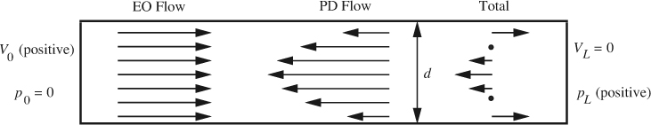
Fig. P12.6 Electroosmotic pressure generation in a closed tube. Directions are shown for a negative wall charge. Left: uniform electroosmotic flow is caused by the electric field. Middle: since the closed tube forces a net mass flow of zero, a pressure is generated at right that causes a parabolic flow from right to left. Right: the net flow is a linear sum of the two flows, which integrates to zero but shows net rightward flow near the wall and net leftward flow at center.
(a) Rework Example 12.2 in the general case. Work in terms of symbols and determine the generated pressure pL in terms of any or all of ζ, ε, μ, V0, L, and d.
(b) If our goal is to generate the largest pressure possible, how should the tube size be selected?
(c) What key parameters are not in this relation?
7. Electrokinetic pressure generation II—D. Expand the analysis in the previous problem to allow the net flow rate (Qtot = Qeo –Qp) to be a variable (the tube is no longer closed). Assume the solution has a conductivity σ, i.e., that the electrical current I through the flow field is given by I = VσA. Derive expressions for the following:
(a) The pressure pL at the outlet as a function of Qtot.
(b) The mechanical output work pLQtot.
(c) The electrical input work V0I.
(d) The thermodynamic efficiency pLQtot/V0I.
(e) Evaluate the thermodynamic efficiency for the conditions in Example 12.2, assuming a conductivity of 100 μS (S = Siemens = ohm –1). Take Qtot to be half of the forward electroosmotic flow in Example 12.2.
8. Ion fluxes and current—E. Consider a 10-cm long channel of diameter d = 50 μm fabricated in glass with a 1-mM solution (M = mol/l) of sodium nitrate (μ = 0.001 kg/m s) at pH = 7 ([H+] = 10 –7, [OH –] = 10 –7). Assume the glass surface has a zeta potential of –60 mV at this condition. Assume a voltage of VL = 1 kV is applied at x = 10 cm and the location x = 0 is grounded (V = 0). Calculate:
(a) The steady-state velocity of all four ions if the fluid velocity is assumed small compared to the ion velocities.
(b) The velocity of the bulk fluid motion—is the assumption made in (a) a good one?
(c) The net charge flux.
(d) The current I and power dissipation rate VLI.
9. Charge density in the electrical double layer—E. The Boltzmann distribution of concentration of an ion in a potential field is given by c = c∞e– qF φ/RT, where q is the ion charge (the valence z = |q|). Assuming that the ions come from NaCl, write the concentration distributions of Na+ and Cl– ions as a function of the potential φ. Given that the local charge density ρe is defined as the sum of the charge density of all species i (ρe = ∑ iqiFci), show that the charge density is:

10. Derivation of electroosmotic flow in the double layer—M. Derive the one-dimensional steady, uniform pressure flow equation in the double layer:
from the relevant full momentum equations (i.e., Navier-Stokes with the Lorentz body force term) and the Poisson equation.
11. Debye lengths—E. Calculate λD for the following conditions (T = 300 K):
(a) Deionized water (z = 1, c = 10 –7 M).
(b) Water at equilibrium with air, which has dissolved CO2 and HCO –3 at equilibrium (z = 1, c = 2 × 10 –6 M).
(c) 1 mM Epsom salts (z = 2, c = 2 × 10 –3 M).
(d) Phosphate-buffered saline, which is often used for biochemical analysis or temporary cell storage (z = 1, c = 0.18 M).
12. Derivation of electroosmotic flow outside the double layer—M. Integrate the one-dimensional boundary-layer equation derived in Problem 12.10 to derive the relation in Eqn. (12.14) for the electroosmotic flow velocity.
13. Nonlinear Poisson-Boltzmann solutions: infinite reservoir—D. Using software such as MATLAB, Excel, or Mathematica, integrate the nonlinear Poisson-Boltzmann equation at c∞ = 10–3 M with boundary conditions: (a)φx= 0 = ζ = –100 mV, (b)φx=∞ = 0, corresponding to a surface in an infinite reservoir of fluid. Take z = 1 and T = 300 K, and plot φ against the distance x from the wall.
14. Nonlinear Poisson-Boltzmann solutions: parallel plates—D. Repeat the previous problem, but use the boundary conditions: (a)φx= 0 = ζ = –100 mV, (b) (dφ/dx)x= 10 nm = 0, corresponding to two parallel plates separated by 20 nm.
15. Streaming potential/streaming current—D. Assume pressure is used to induce laminar flow in a cylindrical tube with diameter 2d and surface potential ζ. Assume d ≫ λD. Since there is a net excess of counterions in the double layer, the net charge flux ∫ uρedA caused by the flow is nonzero, i.e., a net current is induced by this flow. Make the Debye-Huckel approximation and perform the following calculations:
(a) Calculate the net charge flux (streaming current) caused by the flow as a function of the applied pressure, surface potential, viscosity, and permittivity.
(b) Assume the system reaches equilibrium, i.e., that a potential is generated by the net advective charge flux so that the total flux (advective plus conductive) is zero. Assuming that the conductive charge flux is –σAV/L (i.e., that excess conductivity in the double layer can be ignored), show that the resulting potential is given by the Helmholtz-Smoluchowski equation:
16. Electroviscosity I—M. Using Eqns. (12.26) and (12.27), derive a relation for the net flow in a capillary as a function of a, σ, ζ, ε, μ, and dp/dx (assuming thin Debye layers and using the Debye-Huckel approximation). Use this relation to derive a relation for the ratio of the apparent fluid viscosity (i.e., what fluid viscosity would be needed to generate the same net flow rate, ignoring electrokinetic effects) to the true viscosity. Evaluate this ratio for deionized water (σ = 0.1 μS/cm) and a surface potential of –20 mV.
17. Electroviscosity II—E. A simple way to measure the internal diameter of a capillary is to measure the flow rate of fluid with a known viscosity upon application of a known pressure gradient. Suppose you were using a microcapillary system and water to make such a measurement. What would be the simplest and most effective way to ensure that electroviscous effects did not affect your experiment?
18. Scaling laws for electrophoretic separations—E. Assume that two chemical species with electrophoretic mobilities μep1 and μep2 are separated in a channel of length L using an applied field E. How is the resolution affected by the following:
(a) Doubling the electric field at constant L.
(b) Doubling the voltage at constant E.
(c) Doubling the length at constant V.
19. True/false. Check true or false, as appropriate:
(a) Electroosmosis is the motion of fluid caused by an electric field.
T ![]() F
F ![]()
(b) Electroosmotic flow is irrotational everywhere in the flow field.
T ![]() F
F ![]()
(c) Electrophoretic separations can be used to separate uncharged molecules.
T ![]() F
F ![]()
(d) Most of the ions in the electrical double layer are counterions.
T ![]() F
F ![]()
(e) The Debye-Huckel approximation may be made only when the potential is small.
T ![]() F
F ![]()
(f) The electroosmotic velocity is not a function of the size of the channel.
T ![]() F
F ![]()
(g) In a channel with d ≫ λD, there is an electroosmotic velocity at the center of the channel, but there is no electrostatic force there.
T ![]() F
F ![]()
(h) Pressure-driven flows in microchannels are more dispersive than electroosmotic flows.
T ![]() F
F ![]()
(i) Streaming potential measurements require sensitive voltmeters that can measure tiny potentials.
T ![]() F
F ![]()
(j) In an electrolyte solution with a Debye length of 100 nm, particles of 10 nm and particles of 1000 nm will have the same electrophoretic velocity.
T ![]() F
F ![]()
(k) Péclet numbers for microscale flows are always < 1.
T ![]() F
F ![]()
(l) The width of the electrical double layer is independent of the charge of the ions.
T ![]() F
F ![]()