
Chapter 4. Flow in Chemical Engineering Equipment
4.1. Introduction
This chapter concludes the presentation of macroscopic topics, by discussing important applications of fluid mechanics to several chemical engineering processing operations. Since the variety of such operations is fairly large, it will be impossible to cover everything; therefore, the focus will be on a representative set of topics in which the application of fluid mechanics plays a fundamental role in chemical processing. In fact, the general theme is the basic theory that underlies a selection of the so-called “unit operations.” Certain other applications—including those involved in polymer processing, two-phase flow, and bubbles in fluidized beds—depend more on microscopic fluid mechanics for their interpretation, and will be postponed until Chapters 6–11.
In most cases the theory is necessarily simplified, sometimes leading to approximate predictions. However, the reader should thereby gain a knowledge of some of the important issues, which will then enable him or her to make a critical examination of articles in equipment handbooks, process design software, etc., which will generally be needed if serious designs of chemical plants are to be made.
The design and use of process equipment lies at the heart of chemical engineering. Students are encouraged to take every opportunity to see the wide variety of such equipment firsthand, by visiting chemical engineering laboratories, chemical plants, oil refineries, sugar mills, paper mills, glass bottle plants, polymer processing operations, pharmaceutical production facilities, breweries, and waste-treatment plants, etc. Until such visits can be made, an excellent substitute is available on a compact disk produced by Dr. Susan Montgomery and her coworkers.1 The CD can be used on either a PC or a Macintosh computer and consists of many photographs with accompanying descriptions of equipment, arranged under the following headings: materials transport, heat transfer, separations, process vessels, mixing, chemical reactors, process parameters, and process control. The visual encyclopedia is very easy to navigate, and four representative windows are reproduced, with permission, in Figs. 4.1–4.4.
1 Material Balances & Visual Equipment Encyclopedia of Chemical Engineering Equipment, CD produced by the Multimedia Education Laboratory, Department of Chemical Engineering, University of Michigan, Susan Montgomery (Director), 2002.


Fig. 4.3 A typical introductory overview of an item of equipment—cyclones and hydrocyclones in this instance.

4.2. Pumps and Compressors
A fluid may be transferred from one location to another in either of two basic ways:
1. If it is a liquid and there is a drop in elevation, allowing it to fall under gravity.
2. Passing it through a machine such as a pump or compressor that imparts energy to it, typically increasing its pressure (sometimes its velocity), which then enables it to overcome the resistance of the pipe through which it subsequently flows.
Devices that increase the pressure of a flowing fluid usually fall into one of the following two main categories, the first of which is subdivided into two sub-categories:
1. Positive displacement pumps, whose nature is either reciprocating or rotary.
2. Centrifugal pumps, fans, and blowers.
Reciprocating positive displacement pumps. Fig. 4.5 shows how a piston moving to and fro in a cylinder is used for pumping a fluid. The pump is double-acting—the four valves allow fluid to be pumped continuously, whether the piston is moving to the right or the left. The particular instant shown is when the piston is moving to the right. Valve D is closed and fluid is being pumped from the right-hand side of the cylinder through the open valve C to the outlet; simultaneously, valve B is open and fluid is being sucked from the inlet into the left-hand side of the cylinder. In the return stroke, only valves A and D would be open, pumping fluid from the left-hand side to the outlet while filling up the right-hand side from the inlet.

Reciprocating pumps may be used for both liquids and gases, and are excellent for generating high pressures. In the case of gases—for which the pump is called a compressor—there is a significant temperature rise, and intercoolers will be needed if several pumps are used in series in order to produce very high pressures. A variation that avoids friction between the piston and cylinder in order to make a tight seal is to have a pulsating flexible diaphragm. To avoid damage to reciprocating pumps, a provision must be made for automatic opening of a relief valve or recycle line if a valve on the outlet side is inadvertently closed.
Rotary positive displacement pumps. Fig. 4.6 shows how two counter-rotating double lobes inside a casing can be used for boosting the pressure of a fluid between inlet and outlet. A variety of other configurations is possible, such as two triple lobes or two intermeshed gears. The rotary pump is good for handling viscous liquids, but because of the close tolerances needed, it cannot be manufactured large enough to compete with centrifugal pumps for coping with very high flow rates.

Centrifugal pumps. As shown in Fig. 4.7, the centrifugal pump typically resembles a hair drier without the heating element. The impeller usually consists of two flat disks, separated by a distance d by a number of curved vanes, that rotate inside the stationary housing. Fluid enters the impeller through a hole (location “1”) or “eye” at its center, and is flung outward by centrifugal force into the periphery of the housing (“2”) and from there to the volute chamber and pump exit (“3”). Centrifugal pumps are particularly suitable for handling large flow rates, and also for liquids containing suspended solids. The following is only an approximate analysis, the key to which lies in understanding the various velocities at the impeller exit, as follows:
1. The impeller, which has an outer radius r2 and rotates with an angular velocity ω, has a linear velocity u2 = ωr2 at its periphery.

2. Because the fluid is guided by the vanes, which make an angle β with the periphery of the impeller, the relative velocity of the fluid to the impeller, υ2, must also be in this direction.
3. The actual fluid exit velocity, as would be seen by a stationary observer, is c2, the resultant of u2 and υ2.
4. This fluid velocity, c2, has a radially outward component f2, related to the flow rate through the pump by Q = 2πr2df2.
5. Further, the actual velocity c2 has a component w2 tangential to the impeller, and this is known as the “swirl” velocity.
There is a similar set of velocities at the impeller inlet, but they are significantly smaller and may be disregarded in an introductory analysis.
From Eqn. (2.75), the torque needed to drive the impeller and hence the power transmitted to the fluid are:
where m is the mass flow rate through the pump; note the use of the swirl velocity. The additional head Δh imparted to the fluid is the energy it gains per unit mass, divided by the acceleration of gravity:

Within the impeller, this increased head is reflected largely by an increase in the fluid velocity from its entrance value to c2. However, in the volute chamber, there is subsequently a decrease in the velocity, so that the kinetic energy just gained is converted to pressure energy. Thus, the overall pressure increase is:
in which the last approximation—assuming w2 ![]() u2—will be seen from Fig 4.3(d) to be realistic at low flow rates, for which f2 is small. Note that Eqn. (4.2) predicts that Δh should decline linearly with increasing flow rate, which is proportional to f2. This declining head/discharge characteristic is a direct result of the “swept-back” vanes (β < 90°), and is a desirable feature in preserving stability in some pumping and piping schemes; swept-forward vanes are generally undesirable.
u2—will be seen from Fig 4.3(d) to be realistic at low flow rates, for which f2 is small. Note that Eqn. (4.2) predicts that Δh should decline linearly with increasing flow rate, which is proportional to f2. This declining head/discharge characteristic is a direct result of the “swept-back” vanes (β < 90°), and is a desirable feature in preserving stability in some pumping and piping schemes; swept-forward vanes are generally undesirable.
In practice, because of increased turbulence and other losses, Δh is found not to decline linearly with increasing flow rate Q, but in the manner shown in Fig. 4.8. In many cases, the curve is satisfactorily represented by the following relation, where a, b, and n are constants, with n often approximately equal to two:

In addition, the above simplified analysis suggests two dimensionless groups that can be used for all pumps of a given design that are geometrically similar—that is, apart from size, they look alike. If N denotes the rotational speed of the impeller:
The pressure increase at low flow rates is then approximately:

so that the dimensionless group Δp/(ρD2N2) should be roughly constant at low flow rates.
The volumetric flow rate is obtained by multiplying the area πDc1D between the disks of the impeller (the gap width c1D increases linearly with D for a given pump design) by the radially outward velocity c2u2 (this simple theory proposes that the flow rate is roughly proportional to the tangential velocity of the impeller), where c1 and c2 are constants, so that:
Substitution of u2 from (4.5) gives:
Thus, the dimensionless group Q/(ND3) should be roughly constant at low flow rates. In practice, the assumptions made above fail progressively as the flow rate increases. Nevertheless, the two dimensionless groups derived above—for the pressure increase and flow rate—are usually adequate to characterize all pumps of a given design, no matter what the flow rate. Thus, all such pumps can be characterized by the single curve shown in Fig. 4.9; it is the values of the two groups that count, not the individual values of Δp, ρ, D, Q, and N.

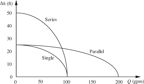
Example 4.1—Pumps in Series and Parallel
For a certain type of centrifugal pump, the head increase Δh (ft) is closely related to the flow rate Q (gpm) by the equation:
where a and b are constants that have been determined by tests on the pump. Two identical such pumps are now connected together, as shown in Fig. E4.1(a), either in series or in parallel.

Fig. E4.1(a) Centrifugal pump arrangements: (i) a single pump, (ii) two in series, (iii) two in parallel.
Derive expressions for the head increases Δhs and Δhp for these two arrangements in terms of the total flow rate Q through them. Also, display the results graphically for the values a = 25 ft and b = 0.0025 ft/(gpm)2.
Solution
When the pumps are in series, the head increases are additive, and the total increase is double that for the single pump:
For the parallel configuration, the flow through each pump is only Q/2. The overall head increase is the same as that for either pump singly:

For the given values of the constants, the results are shown in Fig. E4.1(b). Observe that the series and parallel configurations are useful for allowing operation with increased head and flow rate, respectively.
4.3. Drag Force on Solid Particles in Fluids
Fig. 4.10(a) shows a stationary smooth sphere of diameter D situated in a fluid stream, whose velocity far away from the sphere is u∞ to the right. Except at very low velocities, when the flow is entirely laminar, the wake immediately downstream from the sphere is unstable, and either laminar or turbulent vortices will constantly be shed from various locations around the sphere. Because of the turbulence, the pressure on the downstream side of the sphere will never fully recover to that on the upstream side, and there will be a net form drag to the right on the sphere. (For purely stable laminar flow, the pressure recovery is complete, and the form drag is zero.) In addition, because of the velocity gradients that exist near the sphere, there will also be a net viscous drag to the right. The sum of these two effects is known as the (total) drag force, FD. A similar drag occurs for spheres and other objects moving through an otherwise stationary fluid—it is the relative velocity that counts. And if both the fluid and the solid object are moving with respective velocities Vf and Vs, the drag force is in the direction of the relative velocity Vf – Vs.

In Part II of this book we shall include several examples in which flow patterns can be simulated on the computer—a field known as computational fluid dynamics or CFD. One of these examples appears at the end of Chapter 13, but since it involves flow past a cylinder (somewhat similar to a sphere) it is appropriate to reproduce part of it here, in Fig. 4.10(b). For the case here (Re = 100) the flow is laminar but unsteady, and the diagram shows contours of equal velocities at one instant. As time progresses, the pattern oscillates as the vortices are shed from alternate sides of the cylinder.
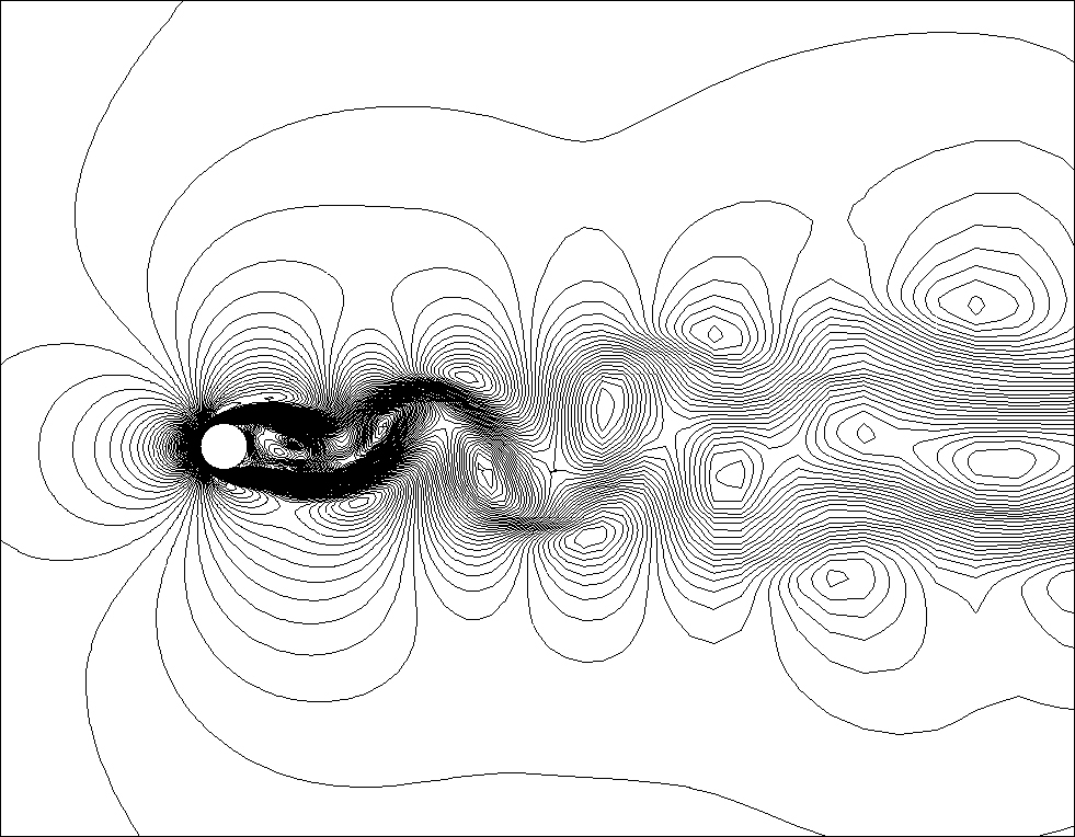
Fig. 4.10(b) Instantaneous velocity contour plots for flow past a cylinder, produced by the FlowLab computational fluid dynamics program at Re = 100. After being shed from the cylinder, the vortices move alternately clockwise (top row) and counterclockwise (bottom row). Courtesy Chi-Yang Cheng, Fluent, Inc.
The analysis is facilitated by recalling that there is a correlation for flow in smooth pipes between two dimensionless groups—the friction factor (or dimensionless wall shear stress) and the Reynolds number:
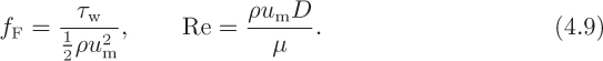
In the same manner, the experimental results for the drag on a smooth sphere may be correlated in terms of two dimensionless groups—the drag coefficient CD and the Reynolds number:

in which Ap = πD2/4 is the projected area of the sphere in the direction of motion, and ρ and μ are the properties of the fluid.
The resulting correlation for the “standard drag curve” (SDC) is shown in Fig. 4.11 for the curve marked ψ = 1 (the other curves will be explained later), in a graph that has certain resemblances to the friction factor diagram of Fig. 3.10. There are at least three distinct regions, as shown in Table 4.1.

Fig. 4.11 Drag coefficients for objects with different values of the sphericity ψ; the curve for ψ = 1 corresponds to a sphere.4

Also, D.G. Karamanev has recalled2 that the entire curve up to the “critical” Reynolds number of about 200,000 can be represented quite accurately by the single equation of Turton and Levenspiel3:

2 Private communication, March 18, 2002.
3 R. Turton and O. Levenspiel, “A short note on the drag correlation for spheres,” Powder Technology, Vol. 47, p. 83 (1986).
Karamanev has also developed an ingenious alternative approach for determining the velocity at which a particle settles in a fluid—presented near the end of this section, together with an important observation on the rise velocities of spheres whose density is significantly less than that of the surrounding liquid.
4 Based on values published in G.G. Brown et al., Unit Operations, Wiley & Sons, New York, 1950, p. 76.
In connection with Fig. 4.11, note:
1. The transition from laminar to turbulent flow is much more gradual than that for pipe flow. Because of the confined nature of pipe flow, it is possible for virtually the entire flow field to become turbulent; however, for a sphere in an essentially infinite “sea” of fluid, it would require an impossibly large amount of energy to render the fluid turbulent everywhere, so the transition to turbulence proceeds only by degrees.
2. The upper limit for purely laminar flow is about Re = 1, in contrast to Re = 2,000 for pipe flow. A prime reason for this is the highly unstable nature of flow in a sudden expansion, which is essentially occurring in the wake of the sphere.
3. There is a fairly sudden downward “blip” in the drag coefficient at about Re = 200,000, because the boundary layer on the sphere suddenly changes from laminar to turbulent. Dimples on a golf ball encourage this type of transition to occur at even lower Reynolds numbers. (Also see Section 8.7 for a more complete explanation.)
For the laminar flow region, the law CD = 24/Re easily rearranges to:
which is known as Stokes’ law,5 which can also be proved theoretically (but not easily!), starting from the microscopic equations of motion (the Navier-Stokes equations).
5 G.G. Stokes, “On the effect of the internal friction of fluids on the motion of pendulums,” Cambridge Philosophical Transactions, Part II, Vol. IX, p. 8 (1850).
Nonspherical particles. For particles that are not spheres, two quantities must first be defined:
1. The sphericityψ of the particle:

It is easy to show that ψ = 1 corresponds to a sphere. Further, sphericities of all other particles must be less than one, because for a given volume a sphere has the minimum possible surface area.
2. The equivalent particle diameter, Dp, defined as the diameter of a sphere having the same volume as the particle.
The corresponding drag coefficient, again defined by Eqn. (4.10), can then be obtained from Fig. 4.11, in which Dp is involved in the Reynolds number, and ψ is the parameter on a family of curves. The value of Ap is nominally the projected area normal to the direction of flow, but this definition lacks precision in the case of a moving particle, which could rotate and lack a constant orientation.
Settling under gravity. Consider the spherical particle of diameter D and density ρs shown in Fig. 4.12, which is settling under gravity in a fluid of density ρf and viscosity μf. A downward momentum balance equates the downward weight of the sphere minus the upward buoyant force, minus the upward drag force, to the downward rate of increase of momentum of the sphere:
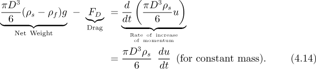

The simplification of constant mass holds in many situations—but not, for example, for a liquid sphere that is evaporating. Integration of (4.14) enables the velocity u to be obtained as a function of time.
Terminal velocity. An important case of Eqn. (4.14) occurs when the sphere is traveling at its steady terminal velocity ut. In this case, the net weight of the sphere is exactly counterbalanced by the drag force and there is no acceleration, so that du/dt = 0 and:
The corresponding drag coefficient is:

A typical problem will specify the value of ut and ask what is the corresponding value of D, or vice versa. Equation (4.16) is not particularly useful, since both the left- and right-hand sides contain unknowns. Alternative forms, whose validity the reader should check, are:


Clearly, the right-hand side of Eqn. (4.17) is independent of ut, and this equation will be useful if ut is sought. In such an event, the product CDRe2 is known and the drag coefficient and Reynolds number (and hence ut) can then be computed with reference to Fig. 4.11. Likewise, the right-hand side of Eqn. (4.18) is independent of D, and this equation will be useful if D is sought. Appropriate values for CD can be obtained from Table 4.1, Fig. 4.11, or Eqn. (4.11).
Karamanev method for rapid calculation of falling and rising terminal velocities. Additionally, D.G. Karamanev has developed a method based on the Archimedes number6:

6 D.G. Karamanev, “Equations for calculation of the terminal velocity and drag coefficient of solid spheres and gas bubbles,” Chemical Engineering Communications, Vol. 147, pp. 75–84 (1996).
in which the absolute value |(ρs – ρf)| allows for the sphere to be either heavier (downwards terminal velocity) or lighter (upwards terminal velocity) than the surrounding fluid. Karamanev shows that the entire curve up to the “critical” Reynolds number of about 200,000 can be represented quite accurately by the single equation:
Thus, if the particle diameter and density and fluid properties are known, the Archimedes number and hence the drag coefficient can be calculated explicitly and quickly, in a form ideally suited for spreadsheet application.
Downward terminal velocity. After Ar and CD have been computed, the terminal velocity for downward settling—that is, when ρs >ρf, is given by:
Upward terminal velocity. For the case in which the solid density is significantly less than that of the surrounding liquid, that is, ρs ≪ ρf, Karamanev summarizes the results of extensive experiments that show:
1. For Re < 135 (corresponding to Ar < 13,000), the SDC (standard drag curve) still applies, and the upward terminal velocity can still be computed from Eqns. (4.20) and (4.21).
2. For Re > 135 (corresponding to Ar > 13,000), the SDC no longer applies. Instead, the drag coefficient shows a sudden upward “jump” to a constant value of CD = 0.95, and this value is then used in Eqn. (4.21) to obtain the upward terminal velocity. At this higher value for CD, the spheres followed a perfect spiral trajectory; the angle between the spiral tangent and the horizontal plane was always very close to 60°. A similar result holds for bubbles rising in liquids.
Applications. Four representative applications of the above theory of particle mechanics are sketched in Fig. 4.13, and are explained as follows:
(a) Separation between particles of different size and density may be achieved by introducing the particles into a stream of liquid that flows down a slightly inclined channel. Depending on the relative rates of settling, different types of particles may be collected in compartments A, B, etc. Clearly, the interaction between particles complicates the issue, but the simple theory presented above should be adequate to make a preliminary design.
(b) Electrostatic precipitators cause fine dust particles or liquid droplets (positively charged, for example) in a fast-moving stream of stack gas to be attracted to a negatively charged electrode. Whether or not the particles actually reach the electrode, from which they can be collected, depends on the drag exerted on them by the surrounding gas.
(c) Spray driers are used for making dried milk, detergent powders, fertilizers, some instant coffees, and many other granular materials. In each case, a solution of the solid is introduced as a spray into the top of a column. Hot air is blown up through the column in order to evaporate the water from the droplets, so that the pure solid can be recovered at the bottom of the column. In this case, the diameter of the particles is constantly changing, and considerations of mass and heat transfer are also needed for a full analysis.

Fig. 4.13 Applications of drag theory: (a) particle separation, (b) electrostatic precipitator, (c) spray drier, and (d) falling-sphere viscometer.
(d) Falling-sphere viscometers can be used for determining the viscosity of a polymeric liquid. By timing the fall of a sphere, chosen to be sufficiently small so that the Stokes’ law regime is observed, the viscosity can be deduced from Eqn. (4.12).
Example 4.2—Manufacture of Lead Shot
Lead shot of diameter d and density ρ is manufactured by spraying molten lead from the top of a “shot tower,” in which the hot lead spheres are cooled by the surrounding air as they fall through a height H, solidifying by the time they reach the cushioning pool of water at the base of the tower. To assist your colleague, who is an expert in heat transfer, derive an expression for the time of fall t of the shot, as a function of its diameter. High accuracy is not needed—make any plausible simplifying assumptions.

Solution
Start with Eqn. (4.14) divided through by πD3ρs/6, and neglect ρf in comparison with ρs:

But, from Eqn. (4.10), since Ap = πD2/4:
so that Eqn. (E4.2.1) becomes:

in which c = 3ρf CD/4 ρsD.
Assume that after a short initial period the drag coefficient is uniform, so that c is approximately constant. Separation of variables and integration between the spray nozzle and the bottom of the tower gives:

or, using Appendix A to determine the integral:
Solution of (E4.2.4) for the velocity gives:
in which:

Integration of Eqn. (E4.2.5) yields:
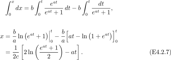
After substituting x = H, Eqn. (E4.2.7) gives the time t taken for the spheres to fall through a vertical distance H. By using standard expansions for ex and ln(1 + x), several lines of algebra show that in the limit as c and/or t become small, Eqn. (E4.2.7) gives:
in which the first term corresponds to a free fall in the absence of any drag, and the second term accounts for the drag.7
7 I thank my colleague Robert Ziff for using Mathematica to check Eqn. (E4.2.8).
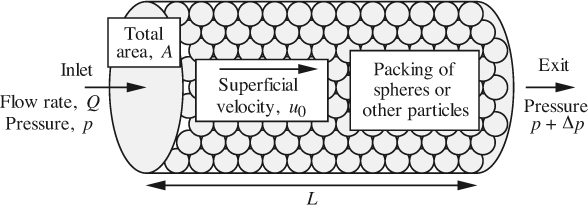
4.4. Flow Through Packed Beds
Flow through packed beds occurs in several areas of chemical engineering. Examples are the flow of gas through a tubular reactor containing catalyst particles, and the flow of water through cylinders packed with ion-exchange resin in order to produce deionized water. The flow of oil through porous rock formations is a closely related phenomenon; in this case, the individual particles are essentially fused together. In all cases, it is usually necessary for a certain flow rate to be able to predict the corresponding pressure drop, which may be substantial, especially if the particles are small.
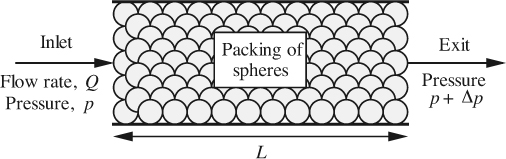
The analysis is performed for the case of a horizontal packed bed, shown in Fig. 4.14, in order to avoid the complicating effect of gravity. Table 4.2 lists the relevant notation.
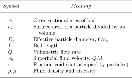
The reader should check that Dp, as defined in Table 4.2, reproduces the actual diameter for the special case of a spherical particle.
The situation may be analyzed to a certain extent by referring to Fig. 4.15(a), which shows the tortuous path taken by the fluid as it negotiates its way through the interstices or pores between the particles. Fig. 4.15(b) shows unit length of an idealized pore, with cross-sectional area A and wetted perimeter P. For a given total volume V, the corresponding hydraulic mean diameter is:


Fig. 4.15 Flow through pores: (a) the tortuous path between particles; (b) an idealized pore (the cross section can be any shape—not necessarily rectangular).
For a horizontal pore, the pressure drop is therefore:

Rearrangement of (4.24) yields:

Thus, theory indicates for turbulent flow, in which fF is essentially constant, that the somewhat unusual dimensionless group on the left-hand side of Eqn. (4.25) should be constant. This prediction is completely substantiated by experiment, and the value of the constant is 1.75.
More generally, however, allowance should be made for a laminar contribution, which will prevail at low Reynolds numbers. The resulting Ergun equation, which is one of the most successful correlations in chemical engineering, is:

in which the Reynolds number is:

The Ergun equation is shown in Fig. 4.16; the limiting cases for low and high Reynolds numbers are called the Blake-Kozeny and Burke-Plummer equations, respectively. Observe that these two forms (one proportional to the reciprocal of the Reynolds number, and the other a constant) are analogous to our previous experience for the friction factor in pipes, first in laminar and then in highly turbulent flow.

Frictional dissipation term for packed beds. So far, we have been concerned only with horizontal beds, for which the overall energy balance is:
Thus, from Eqn. (4.22), the frictional dissipation term per unit mass flowing is:

Although F from Eqn. (4.29) has been derived for the horizontal bed (in order to isolate the purely frictional effect), this relation can then be substituted into the appropriate energy balance for an inclined or vertical packed bed.
d’Arcy’s law. The above theory can be applied to a consolidated or porous medium, in which the particles are fused together, such as would occur in a sandstone rock formation through which oil is flowing. Since the flow rate is likely to be small, and again considering horizontal flow (that is, ignoring changes in pressure caused by hydrostatic effects), the turbulent term in Eqn. (4.26) can be neglected as a good approximation, giving:

Rearranging, the superficial velocity is given by d’Arcy’s law:
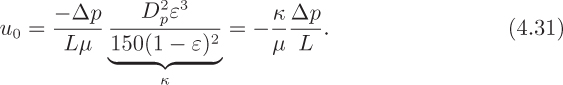
Note that since the concept of an individual particle diameter no longer exists, the fraction κ shown in Eqn. (4.31) with an underbrace is collectively considered to be another physical property of the porous medium, known as its permeability. If u0 is measured in cm/s, Δp in atm, μ in cP, and L in cm, the unit of permeability is known as the darcy, which is equivalent to:

The differential form of d’Arcy’s law in one dimension is:
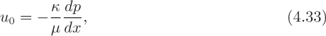
which is a classical type of relation, in which a flux (here a volumetric flow rate per unit area) is proportional to a conductivity (κ/μ) times a negative gradient of a potential driving force (dp/dx). A more general, vector form of d’Arcy’s law, v = –(κ/μ)∇p, is given in Eqn. (7.76).
Example 4.3—Pressure Drop in a Packed-Bed Reactor
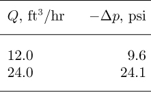
A liquid reactant is pumped through the catalytic reactor shown in Fig. E4.3, which consists of a horizontal cylinder packed with catalyst spheres of diameter d1 = 2.0 mm. Tests summarized in Table E4.3 show the pressure drops –Δp across the reactor at two different volumetric flow rates Q.
If the maximum pressure drop is limited by the pump to 50 psi, what is the upper limit on the flow rate? After the existing catalyst is spent, a similar batch is unfortunately unavailable, and the reactor has to be packed with a second batch whose diameter is now d2 = 1.0 mm. What is the new maximum allowable flow rate if the pump is still limited to 50 psi?
Solution
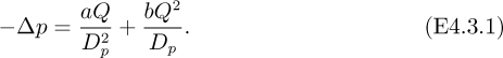
From Eqn. (4.29), for constant μ, L, ε, and ρ, noting that u0 is proportional to Q and that all conversion factors can be absorbed into the constants a and b:
Inserting values from Table E4.3:

Solution of these two simultaneous equations gives a = 2.38 and b = 0.0340, so the maximum flow rate Qmax is given by the quadratic equation:
from which Qmax = 39.5 ft3/hr.
For the new catalyst, Dp is now only 1.0, so the new maximum flow rate obeys the equation:
yielding Qmax = 16.9 ft3/hr. Note that the flow rate declines appreciably for the finer size of packing.
4.5. Filtration
Introduction and plate-and-frame filters. A filter is a device for removing solid particles from a fluid stream (often from a liquid). Examples are:
1. In the paper industry, to separate paper-pulp from a water/pulp suspension.
2. In sugar refining, either to clarify sugar solutions or to remove wanted saccha-rates from a slurry.
3. In the recovery of magnesium from seawater, to separate out the insoluble magnesium hydroxide.
4. In metallurgical extraction, to remove the unwanted mineral residues from which silver and gold have been extracted by a cyanide solution.
5. In automobiles, to clean oil and air.
6. In municipal domestic water plants, to purify water.
The basic elements of a filter are shown in Fig. 4.17.
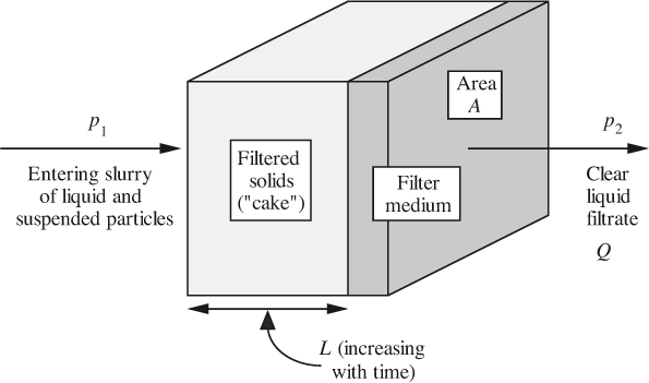
A slurry, containing liquid and suspended particles at an inlet pressure p1, flows through the filter medium, such as a cloth, gauze, or layer of very fine particles. The clear liquid or filtrate passes at a volumetric rate Q through the medium into a region where the pressure is p2, whereas the suspended particles form a porous semisolid cake of ever-increasing thickness L.
A plate-and-frame filter consists of several such devices operating in parallel. The cloth is supported on a porous metal plate, and successive plates are separated by a frame, which also incorporates various channels to supply the slurry and remove the filtrate. When the cake has built up to occupy the entire space between successive plates, the filter must be dismantled in order to remove the cake, wash the filter, and restart the operation. Detailed views are given in Fig. 4.18.

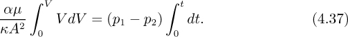
In many cases, the resistance of the filter medium can be neglected. If A is the area of the filter, and if V denotes the total volume of filtrate passed since starting with L = 0 at t = 0, d’Arcy’s law gives:

But the thickness of the cake increases linearly with the volume of filtrate, so that:
in which α is the volume of cake deposited by unit volume of filtrate. Hence,
Depending largely on the characteristics of the pump supplying the slurry under pressure, two principal modes of operation are now recognized.
1. Constant-pressure operation occurs approximately if a centrifugal pump, not operating near its maximum flow rate, is employed. With the pressure drop (p1 – p2) thereby held constant, integration of Eqn. (4.36) up to a time t yields:
That is, the volume of filtrate varies with the square root of elapsed time according to:
2. Constant flow-rate operation occurs when a positive displacement pump is used, in which case the inlet pressure simply adjusts to whatever is needed to maintain the flow rate Q at a steady value. Since V = Qt, differentiation yields:
Substitution for dV/dt from Eqn. (4.36) then gives the relation between the pressure drop and the flow rate:
Rotary vacuum filters. A disadvantage of the plate-and-frame filter is its intermittent operation—it must be dismantled and cleaned when the cake has built up to occupy the entire space between the plates. Generally, chemical engineers prefer continuous processing operations, which in the case of filtration can be achieved by the rotary vacuum filter shown in Fig. 4.19.

The slurry to be filtered is supplied continuously to a large bath, in which a partly submerged perforated drum is rotating slowly at an angular velocity ω.
The drum is divided internally into several separate longitudinal segments, and by a complex set of valves (not shown here) each segment can be maintained either below or above atmospheric pressure. Thus, a partial vacuum applied to the submerged segments causes filtration to occur, the cake building up on the surface of the drum, and the filtrate passing inside the drum, where it is removed at one end by piping (also not shown). The partial vacuum also causes the wash water to pass through the cake, and it too is collected by additional piping at one end of the drum. The washed cake is finally detached by a scraper or “doctor knife,” assisted by a small positive pressure inside the segment just approaching the scraper.
The analysis of the rotary vacuum filter is similar to that of the plate-and-frame filter, in which the time of operation is the period for one complete rotation (2π/ω) multiplied by the fraction of segments under vacuum that are in contact with the slurry. The operation is essentially constant pressure, because of the steady vacuum inside the drum relative to the atmosphere.
Centrifugal filters. One type of centrifugal filter is shown in Fig. 4.20. It consists of a cylindrical basket with a perforated vertical surface (as in a washing machine), covered with filter cloth, that is rotated at a high speed. Slurry sprayed on the inside is flung outwards by centrifugal action and soon starts to deposit a lining of cake on the inside of the wall. The filtrate discharges through the perforations and is collected in an outer casing. After a suitable amount of cake has been deposited, the slurry feed is stopped and the basket is slowed down, during which period the cake is washed and scraped off the wall. The cake is then deposited into a receptacle through openable doors in the base.

The analysis of the centrifugal filter follows standard lines. In the slurry, the pressure increases because of centrifugal action, from atmospheric pressure at r = r1 to a maximum at r = a. In the cake, centrifugal action again tends to increase the pressure, but friction dissipates this effect, so that the discharge at r = r2 has reverted to atmospheric pressure. The liquid will “back up” to the appropriate radius r1 that suffices to provide the necessary driving force to overcome friction in the cake.
The basic equations governing pressure in the slurry and in the cake are:
Here, κ is the cake permeability, and the superficial velocity for d’Arcy’s law has been recognized as u0 = Q/(2πrH), where Q is the filtrate flow rate. Unless otherwise stated, the resistance of the filter medium is usually neglected, and the slurry and filtrate densities ρS and ρF have essentially the same value, ρ. The slurry equation can be integrated forward, from r1, where p = 0, to give the pressure in the slurry. The cake equation can be integrated backward, from r2, where p = 0, to give the pressure in the cake. The two expressions for the pressure must match, of course, at the slurry/cake interface, r = a.
Considerations of the rate of cake deposition show that the inner radius a of the cake gradually decreases as solids are deposited, according to:
in which α is the volume of cake per unit volume of filtrate.
4.6. Fluidization
Fig. 4.21(a) illustrates upwards flow of a fluid through a bed of initial height h0 that is packed with particles of diameter Dp. Fig. 4.21(b) shows the relation between the actual bed height h and the superficial velocity u.

Fig. 4.21 Fluidization: (a) upward flow through a packed bed, and (b) variation of bed height with superficial velocity.
For low u, h is almost unchanged from its initial value. However, as u is increased, the pressure drop p1 – p2 also increases, and will eventually build up to a value that suffices to counterbalance the downward weight of the particles. At this point, when u has reached the incipient fluidizing velocity u0, the particles are essentially weightless and will start circulating virtually as though they were a liquid. Further increases in u will cause the bed to expand (still in a fluidized state), whereas the pressure drop now increases only slightly.
Fluidized beds are excellent for providing good contact and mixing between fluid and solid, as is required in some catalytic reactors. (See also Section 10.6 for further details of fluidized beds—particularly relating to particulate and aggregative modes of operation.) The value of the incipient fluidizing velocity may be obtained by the following treatment. An energy balance applied between the bed inlet and exit gives:
The pressure drop can now be extracted and equated to the downward weight of particles and fluid per unit area:

where ε0 is the void fraction when the bed is on the verge of fluidization. Isolation of the frictional dissipation term gives:
But F is given by the right-hand side of Eqn. (4.29):

Thus, from Eqns. (4.45) and (4.46), after canceling (1 – ε0)h0, the incipient fluidizing velocity u0 is given in terms of all other known quantities by:

A much more complete discussion of fluidized beds is given in the latter part of Chapter 10.
4.7. Dynamics of a Bubble-Cap Distillation Column
The basic principles learned so far can be employed to insure the satisfactory operation of a distillation column, a cross section of which is shown in Fig. 4.22(a). Such a column is used to separate or fractionate a mixture, based on the different boiling points or volatilities of the components in a feed stream, which could typically consist of ethanol and water, or a mixture of “light” (low boiling point) and “heavy” (high boiling point) hydrocarbons. The most volatile components become concentrated toward the top of the column, and the least volatile toward the bottom.

Fig. 4.22 Distillation column: (a) overview; (b) detail of liquid on three successive trays; (c) plan of one tray.
The essential parts of the column are:
1. A reboiler, typically steam-heated, that boils the liquid from the bottom of the column, part of which is withdrawn as the bottoms product, rich in the heavy components. The rest of the liquid is vaporized and returned to the column.
2. A series of trays on which the liquid mixture is boiling. Vapor somewhat enriched in the lighter components rises to the tray above, and liquid somewhat enriched in the heavier components falls to the tray below.
3. A condenser, typically cooled by water, liquefies the vapor from the top tray. Part of the liquid is returned to the top tray as reflux, and the rest is withdrawn as the overhead product, rich in the light components.
As seen from Fig. 4.22(b), boiling liquid is continuously spilling over a weir at one side of every tray, from there flowing via a downcomer and through a constriction to the tray below. Vapor, boiling from the liquid on each tray, is simultaneously flowing upward through bubble caps (which act as liquid seals, and only a few of which are shown in the diagram) into the boiling liquid on the tray immediately above. We wish to insure that the arrangement is stable.
Adopt the notation shown in Table 4.3. The pressure of the vapor leaving a tray must be high enough to overcome the hydrostatic pressure of the liquid on the tray above, and hence to enable the vapor to flow through the bubble caps. The excess pressure required is approximately:

which corresponds to a liquid head of (d + D). A further refinement, not made here, would be to include a small extra pressure loss as the vapor follows the tortuous path through the bubble cap.
Next consider the flow of the liquid over the weir, where the pressure is everywhere uniform (equal to p, for example). Liquid at a depth y below the upper surface will have come from an upstream location where the pressure is p + ρLgy and, on account of the greater depth, the velocity is smaller and may be neglected. Thus, applying Bernoulli’s equation, the velocity at the weir location is approximately:
Integration gives the liquid flow rate:

Here, a coefficient of discharge CD, typically about 0.62, has been introduced to allow for deviations from the theory, mainly because of a further contraction of the liquid stream as it spills over the weir.
The available driving head h has to overcome two resistances:
1. The head (d + D) needed to cause the gas to flow.
2. The loss of kinetic energy as the liquid jet at the bottom of the downcomer is dissipated as it enters the tray.
Thus, equating these two effects:

For sufficiently high liquid flow rates, the level in any downcomer can only back up to the level of the tray above before it starts interfering with the flow from the weir above. In such event, the tray spacing is the sum of the three individual heights shown in Fig. 4.22(b):
Under these conditions, also using Eqn. (4.51):

Note from Eqn. (4.50) that:
and eliminate the unknown d from Eqns. (4.53) and (4.54), finally giving:
Hence, the maximum liquid flow rate Lmax under which the column can operate successfully is given by Eqn. (4.55). Any attempt to increase the liquid flow rate beyond Lmax will cause liquid to occupy the entire column, a phenomenon known as “flooding.” Under these circumstances, there is no space left for the vapor, and normal operation as an effective distillation column ceases.
4.8. Cyclone Separators
Solid particles—even dust—may be separated from a fluid stream—usually a gas—by means of a cyclone separator, the elements of which are shown in Fig. 4.23. The notation for the analysis appears in Table 4.4.

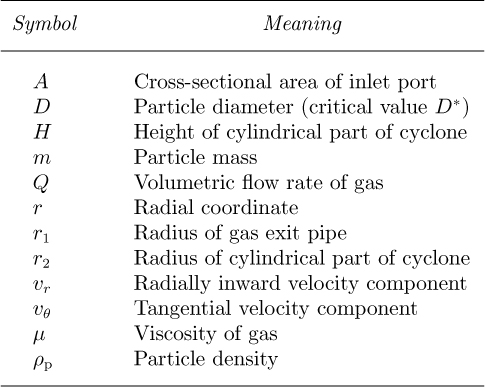
A volumetric flow rate Q of particle-containing gas enters tangentially through an inlet port, of cross-sectional area A, into the top of a virtually empty cylinder, of radius r2. The swirling motion tends to cause the particles to be flung out to the wall of the cyclone, from which they subsequently fall by gravity into the lower conical portion for collection. The particle-free gas discharges upward through a large pipe of radius r1.
The effectiveness of the cyclone may be approximated by a simple analysis, by considering both the centrifugal force and fluid drag acting on the particles. The velocity of the gas in the cylindrical portion has three components:
1. An inward radial velocity, υr, as the gas travels from the inlet to the exit. For a cylinder height H, continuity gives as a first approximation:
2. A tangential velocity, υθ, which—again to a first approximation—is inversely proportional to the radius, as in a free vortex (see Section 7.2). Since the inlet value of υθ is Q/A at a radius r2, its value at any smaller radius r is:
Equation (4.57) also follows from the principle of conservation of angular momentum (see Section 2.6), in which ωr2 is constant, where ω = υθ/r is the angular velocity.
3. A vertical component, υz, first descending from the inlet (even into the conical portion) and eventually changing direction and rising into the gas exit. In the present simplified analysis, υz will be ignored, but it could be accommodated by treating the situation as a potential flow problem according to the methods given in Chapter 7, in which case a relatively complex computer-assisted numerical solution would be needed to obtain a proper description of the entire flow pattern.
Consider the forces acting on a representative particle of density ρp, which is assumed to be so small that Stokes’ law applies. (For larger particles, an appropriate drag coefficient would have to be incorporated into the analysis.) A particle will remain at a radial location r when the radially outward centrifugal force is counterbalanced by an inward drag, giving:
Substitute for the two velocity components from Eqns. (4.56) and (4.57), and note the particle mass is m = ρpπD3/6. The inward drag and outward centrifugal force will then be in balance at a radius r for a particle of diameter:
Taking the most pessimistic view, the diameter D* of the largest particle that we are sure will not be attracted toward the gas exit is obtained by setting r = r2:

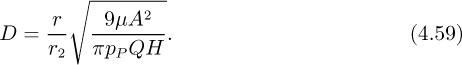
A particle whose diameter equals or exceeds D* will be trapped at the outer wall and will fall by gravity so that it is separated from the gas. However, a particle with D < D* will tend to be dragged toward the exit tube and may not be separated from the gas. Observe that small values of A and large values of Q will serve to reduce D* and hence enable smaller particles to be collected.
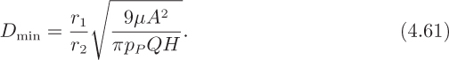
If we set r = r1 in Eqn. (4.59), we obtain a diameter Dmin below which all particles will tend to reach the exit tube:
We emphasize that motion in the vertical direction has been neglected and that the above results are only approximate.
4.9. Sedimentation
Section 4.3 dealt with the relative motion of a single particle in a fluid. In particular, a method was discussed for obtaining the terminal velocity ut of a single particle settling under gravity in a fluid. Some chemical engineering operations involve many such particles that are sufficiently close together so that the previous theory no longer applies.
Fortunately, the Richardson/Zaki8 correlation is available to give the settling velocity u of a group of particles as a function of the void fraction ε (the fraction of the total volume that is occupied by the fluid):
8 J.F. Richardson and W.N. Zaki, “Sedimentation and fluidisation,” Transactions of the Institution of Chemical Engineers, Vol. 32, p. 35 (1954).
Here, the value of exponent n is primarily a function of the Reynolds number Re = ρf uD/μ, as shown in Table 4.5. (Richardson and Zaki also found that n depends to a much smaller extent on the ratio of the particle diameter to that of the containing vessel—a fact that can reasonably be ignored here.) Note that Eqn. (4.62) correctly reduces to u = ut (the terminal velocity of a single particle) when the void fraction is ε = 1.

Now examine the sedimentation in a liquid of a large cluster of particles in a container, as shown in Fig. 4.24. Initially, the particles are uniformly distributed throughout the liquid, as in (a). At some later time, as in (b), they will tend to congregate toward the bottom of the container. That is, the void fraction will vary from a relatively high value at the top of the container to a relatively low value at the bottom. We wish to derive the differential equation that governs the variation of the void fraction ε with both height z and time t.

Consider a differential element of cross-sectional area A and height dz, as in Fig. 4.24(d). Since the fraction of volume occupied by the particles is (1 – ε), the rate at which particle volume leaves the element through its lower surface is u(1 – ε) per unit area. The rate at which particle volume enters the element through its upper surface is differentially greater, as shown in the diagram. Next, equate the net rate of particle volume entering the element to the rate of increase of particle volume inside the element, giving:
Substitution of the particle velocity from Eqn. (4.62) yields the following differential equation:
Unfortunately, there is no ready analytical solution of Eqn. (4.64), but—starting at t = 0 with a known initial distribution of ε—numerical methods could be employed to determine how the void fraction ε varies with elevation z and time t.
4.10. Dimensional Analysis
Dimensional analysis is important because it enables us to express relations between variables—whether analytical solutions or experimental correlations—very concisely. Instead of attempting to establish a relation that may involve several variables independently, a much simpler relation is typically established between a relatively small number of groups of variables. With proper planning, the technique also often reduces the number of experiments that are needed in certain investigations. There are two main approaches in determining the appropriate dimensionless groups, depending whether or not an analytical solution or similar model is already available.
1. Four examples of the first approach, which rearranges an existing solution into dimensionless groups, are available from material already studied:
(a) Consider Eqn. (4.38), for the constant-pressure operation of a batch filter:
Rearrangement in terms of a dimensionless group Π, gives:

which states that no matter what the individual values of V, μ, etc., the performance of all filters can be expressed by the equation:
(b) The shape of the free surface of a rotating liquid is:
Observe that both the group of variables on the left-hand side, and the fraction on the right-hand side, are dimensionless.
(c) For the evacuation of the tank in Example 2.1, the dimensionless pressure ratio p/p0 is a function of the dimensionless time vt/V.
(d) Finally, consider Eqn. (3.40), the semi-empirical Blasius relation that expresses the dimensionless wall shear stress for turbulent flow in a smooth pipe in terms of the (dimensionless) Reynolds number:
which can be written out fully as:

Again note that the correlation in terms of the dimensionless groups is much more concise than that with the individual variables.
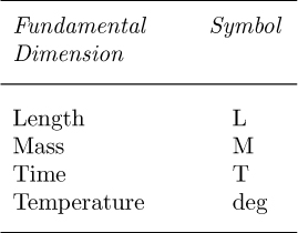
2. The second approach, in which appropriate dimensionless groups have to be found, is useful when there is no existing model or solution. First, four fundamental dimensions are identified, as shown in Table 4.6; temperature is given for completeness, but is generally unnecessary for most fluid mechanics work.
Now express the dimensions of other variables, known as derived quantities, in terms of the fundamental dimensions, as shown in Table 4.7. There, “deg” denotes Kelvins, degrees Fahrenheit, etc., as appropriate.

Wall shear stress for pipe flow. The general approach is illustrated for a specific case. Assume, based on experience, that the wall shear stress τω in pipe flow is likely to depend only on the distance x from the inlet, D, um, ρ, μ, and the wall roughness ε. That is,
where ψ denotes a functional dependency—as yet unknown. Hence, there exists some relation between all the seven variables, written as:
Observe that the functions ψ are different in (4.68) and (4.69); since both are unknown, it is pointless to use a different symbol each time, so ψ is really a “generic” functional dependency. The dimensions of the various quantities are given in Table 4.8.

Next, choose as many primary quantities as there are fundamental dimensions (three in this case), as long as they contain all the relevant fundamental dimensions explicitly among them. For example, we can choose D, ρ, and um (L, M/L3, and L/T) as primary quantities because the dimensions L, M, and T are available in D, ρD3, and D/um. However, x, D, and μ (L, L, M/LT) would be an improper choice because there is no combination of these variables that generates M and T individually (the ratio M/T persists). Having chosen D, ρ, and um, form dimensionless ratios, given the general symbol Π, for the remaining quantities τω, μ, x, and ε, as follows:
For τω, the first group is formulated as:
Next, choose the exponents a, b, and c so that Π1 is dimensionless:

Considering each of the fundamental dimensions M, L, and T in turn, three simultaneous equations result:

for which the solution is a = 0, b = 1, and c = 2. The first dimensionless group is therefore:
A similar procedure for μ, x, and ε gives the following dimensionless groups:
It is then a fundamental postulate, known as the Buckingham Pi Theorem, that there exists some relation among the dimensionless groups thus formed:
Note that the original problem of developing a correlation among seven variables has now been simplified enormously to that of finding a correlation among just four dimensionless groups.
Substituting for the Π groups in (4.75):

Since the wall shear stress is the quantity of greatest interest, an obvious rearrangement of (4.76) is:

That is, given experimental values of τω, x, D, um, ρ, μ, and ε, dimensional analysis indicates that all pipe flow data can be correlated by a series of plots, each for a known value of x/D, of ![]() versus ρumD/μ, with ε/D as a parameter. This conclusion is completely verified and quantified by experiment. In practice, except near the pipe entrance in laminar flow, x/D is found to be of secondary importance only and is often ignored, in which case the friction factor plot of Fig. 3.10 is obtained.
versus ρumD/μ, with ε/D as a parameter. This conclusion is completely verified and quantified by experiment. In practice, except near the pipe entrance in laminar flow, x/D is found to be of secondary importance only and is often ignored, in which case the friction factor plot of Fig. 3.10 is obtained.
Table 4.9 gives the dimensionless groups (including those involved in heat transfer) of greatest interest to the chemical engineer. In almost all cases, each group corresponds to the ratio of two competing effects, N (numerator) divided by D (denominator). For example, the Reynolds number is the ratio of an inertial effect, ![]() , to a viscous effect, μum/D.
, to a viscous effect, μum/D.

The following terms are often used in dimensional analysis:
1. Dynamical similarity, which indicates equality of the appropriate dimensionless groups in two cases that are being compared. Translated in terms of a Reynolds number, for example, this means that the balance between inertial and viscous forces is the same in the two situations.
2. Geometrical similarity, which means that except for size, the geometrical appearance is the same. For example, if the performance of a full-size oceangoing oil tanker were to be predicted by performing tests on a scale model, then—fairly obviously—the model should be that of an oil tanker and not a rowing boat!
Example 4.4—Thickness of the Laminar Sublayer
Fig. E4.4 shows an idealized version of the velocity profile for turbulent flow in a pipe of diameter D. The central turbulent core, which occupies almost all of the cross section, has a uniform (time-averaged) velocity u. Additionally, there is a thin laminar sublayer of thickness δ, adjacent to the wall, in which the velocity builds up linearly from zero at the wall to u at the junction with the turbulent core.

From experiment, the dimensionless shear stress (friction factor) is found to be constant at high Reynolds numbers, independent of the flow rate:
Determine, in dimensionless terms, how the thickness δ of the laminar sublayer varies with the velocity u.
Solution
The wall shear stress is the product of the viscosity and the velocity gradient in the laminar sublayer:
Elimination of τω between Eqns. (E4.4.1) and (E4.4.2) gives:
By solving for δ and dividing by D, Eqn. (E4.4.3) yields the desired result, as a relation between two dimensionless groups:
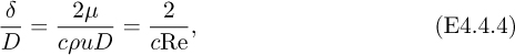
in which Re is the Reynolds number, ρuD/μ. Thus, the thickness of the laminar sublayer is inversely proportional to the Reynolds number. That is, as Re increases, the flow in the central portion becomes more turbulent, confining the laminar sublayer to a thinner region next to the wall. Eqn. (E4.4.4) enables δ/D to be estimated: for example, taking c = fF = 0.00325 and Re = 50,000 as representative values, we find that δ/D = 0.0123.
Finally, note that the present result compares favorably with Eqn. (3.62), which holds if a more sophisticated model (the one-seventh power law) is taken for the velocity profile in the turbulent core:
Problems for Chapter 4
Unless otherwise stated, all piping is Schedule 40 commercial steel, and the properties of water are: ρ = 62.3 lbm/ft3, μ = 1.0 cP.
1. Pumping air and oil—E. Ideally, what pressure increases (psi) could be expected across centrifugal pumps of 6-in. and 12-in. impeller diameters when pumping air (ρ = 0.075 lbm/ft3) and oil (ρ = 50 lbm/ft3)? Four answers are expected. The impellers run at 1,200 rpm.
2. Pump and pipeline—M. The head/discharge curve of a centrifugal pump is shown in Fig. P4.2. The exit of the pump is connected to 1,000 ft of nominal 2-in. diameter horizontal pipe (D = 2.067 in.). What flow rate (ft3/s) of water can be expected? Assume atmospheric pressure at the pump inlet and pipe exit, and take fF = 0.00475.

3. Pump scale model—E. A centrifugal pump operating at 1,800 rpm is to be designed to handle a liquid hydrocarbon of specific gravity 0.95. To check its performance, a half-scale model is to be tested, operating at 1,200 rpm, pumping water. The scale model is found to deliver 200 gpm with a head increase of 22.6 ft. Assuming dynamical similarity (equality of the appropriate dimensionless groups), what will be the corresponding flow rate (gpm) and head increase (ft) for the full-size pump?
4. Dimensional analysis of pumps—M. Across a centrifugal pump, the increase in energy per unit mass of liquid is gΔh, where g is the gravitational acceleration and Δh is the increase in head. This quantity gΔh (treat the combination as a single entity) may be a function of the impeller diameter D, the rotational speed N, and liquid density ρ (but not the viscosity), and the flow rate Q. Perform a dimensional analysis from first principles, in which gΔh and Q are embodied in two separate dimensionless groups.
A centrifugal pump operating at 1,450 rpm is to be designed to handle a liquid hydrocarbon of s.g. (specific gravity) 0.95. To predict its performance, a half-scale model is to be tested, operating at 725 rpm, pumping a light oil of s.g. 0.90. The scale model is found to deliver 200 gpm with a head increase of 20 ft. Assuming dynamical similarity, what will be the corresponding flow rate and head increase for the full-size pump?
5. Pumps in series and parallel—M. Two different series/parallel arrangements of three identical centrifugal pumps are shown in Fig. P4.5. The head increase Δh across a single such pump varies with the flow rate Q through it according to:
Δh = a – bQ2.

Derive expressions for the head increases Δh(a) and Δh(b), in terms of a and b and the total flow rate Q, for these two configurations. Sketch your results on a graph, also including the performance curve for the single pump. Note: In case (b), it might be possible for the two pumps in series in the one branch to overpower the third pump and cause a reversal of flow through it. Such a possibility is prevented by the check valve, which permits only forward flow.
6. Solar-car performance—E. A solar car has a frontal area of 12.5 ft2 and a drag coefficient of 0.106.9 If the electric motor is delivering 1.2 kW of useful power to the driving wheels, estimate the corresponding maximum speed near Alice Springs in the Australian “outback.”
9 This problem was inspired by the success of the Sunrunner solar-powered car designed and built in 12 months by University of Michigan engineering students. In General Motors Sunrayce USA in July 1990 against 31 other university teams, Sunrunner placed first in an 11-day race from Epcot Center, Florida, to the General Motors Technical Center in Warren, Michigan. In October 1990, Sunrunner was again first among university teams (and third overall among 36 contestants, including professional teams) in the World Solar Challenge race from Darwin to Adelaide. Sunrunner’s motor was rated at 3 HP, so it could actually deliver more than 1.2 kW if it drew additional electricity from the storage battery.
7. Terminal velocity of hailstones—M. Occasionally, 1.0-in. diameter hailstones fall in Ann Arbor. What is their terminal velocity in ft/s? Take CD = 0.40 as a first approximation and assume anything else that is reasonable. Data: densities (lbm/ft3): ice, 57.2; air, 0.0765; viscosity of air: 0.0435 lbm/ft hr.
8. Hot-air balloon emergency—E. Uninflated, the total mass of a hot-air balloon, including all accessories and the balloonist, is 500 lbm. Inflated, it behaves virtually as a perfect sphere of diameter 80 ft, and rises in air at 50 °F, whose density is 0.0774 lbm/ft3. Unfortunately, the burner fails, the air in the balloon cools, the balloon loses virtually all of its buoyancy, and soon reaches a steady downward terminal velocity, fortunately still retaining its spherical shape.
The balloonist is yourself. Having taken a fluid mechanics course, you are accustomed to making quick calculations, and are prepared to endure a 10 ft/s crash, but will use a parachute otherwise. You know that for very high Reynolds numbers the drag coefficient is constant at about 0.44. Based on the above, would you use the parachute? Why?
9. Viscosity determination—M. This problem relates to finding the viscosity of a liquid by observing the time taken for a small ball bearing to fall steadily through a known vertical distance in the liquid.
A stainless steel sphere of diameter d = 1 mm and density ρs = 7,870 kg/m3 falls steadily under gravity through a polymeric fluid of density ρf = 1,052 kg/m3 and viscosity μ = 0.1 kg/m s (Pa s). What is the downward terminal velocity (cm/s) of the sphere?
10. Ascending hot-air balloon—M. A spherical hot-air balloon of diameter 40 ft and deflated mass 500 lbm is released from rest in still air at 50 °F. The gas inside the balloon is effectively air at 200 °F. Assuming a constant drag coefficient of CD = 0.60, estimate:
(a) The steady upward terminal velocity of the balloon.
(b) The time in seconds it takes to attain 99% of this velocity.
The density of air (lbm/ft3) is 0.0774 at 50 °F and 0.0598 at 200 °F. The table of integrals in Appendix A should be helpful.
11. Baseball travel—M. The diameter of a baseball is 2.9 in, and its mass is 0.32 lbm. If the drag coefficient is CD = 0.50, obtain an expression in terms of u2 for the drag force of the air (ρ = 0.075 lbm/ft3) on the baseball. If it leaves the pitcher on the mound at 100 mph, estimate its velocity by the time it crosses the plate, 60 ft away. Hint: Eventually use the relation u = dx/dt to change the standard momentum balance into a differential equation in which the variables are u and x (not u and t), before integrating.
12. Packed bed flow—M. Outline briefly the justification for supposing that the energy-equation frictional dissipation term for flow with superficial velocity u0 through a packed bed of length L is of the form:
in which a and b are constants that depend on the nature of the packing and the properties of the fluid flowing through the bed.
As shown in Fig. P4.12, a bed of ion-exchange resin particles of depth L = 2 cm is supported by a metal screen that offers negligible resistance to flow at the bottom of a cylindrical container. Liquid (which is essentially water with μ = 1 cP and ρ = 1 g/cm3) flows steadily down through the bed. The pressures at both the free surface of the water and at the exit from the bed are both atmospheric.

The following results are obtained for the liquid height H as a function of superficial velocity u0:
First, obtain the values of the constants a and b for the packed bed. (Hint: Perform overall energy balances between the liquid entrance and the packing exit, ignoring any exit kinetic energy effects.) Second, what is the d’Arcy’s law permeability (cm2) for the packed bed at very low flow rates?
Third, a prototype apparatus is to be constructed in which the same type of ion-exchange particles are contained between two metal screens in the form of a hollow cylinder of outer radius 5 cm and inner radius 0.5 cm. What pressure difference (bar) is needed to effect a steady flow rate of 10 cm3/s of water per cm length of the hollow cylinder? (If needed, assume the flow is from the outside to the inside.) Hint: Start from equation (P4.12.1) and obtain a differential equation that gives dp/dr.
13. Performance of a water well—M. Fig. P4.13 shows the horizontal cross section of a well of radius r1 in a bed of fine sand that produces water at a volumetric flow rate Q per unit depth and at a pressure p1. The water flows radially inwards from the outlying region, with symmetry about the axis of the well. A pressure transducer enables the pressure p2 to be monitored at a radial distance r2.

Prove that the superficial velocity u0 radially inwards of the water varies with radial position r according to:
The following data were obtained for r1 = 3 in. and r2 = 300 in.:
Calculate p2 – p1 for Q = 300 gpm/ft. Also, for Q = 100 gpm/ft and p1 = 0 psi, what would the pressure be at r = 6 in?
Start from the Ergun equation, which has the following appropriate form:

14. Pressure drop in an ion-exchange bed—E. A horizontal water purification unit consists of a hollow cylinder that is packed with ion-exchange resin particles. Tests with water flowing through the unit gave the following results:
If the available pump limits the pressure drop over the unit to a maximum of 54 psi, what is the maximum flow rate of water that can be pumped through it?
15. Plate-and-frame filter—M. The following data were obtained for a plate-and-frame filter of total area A = 500 cm2 operating under a constant pressure drop of Δp = 0.1 atm:
The filtrate is essentially water. The volume of the cake is one-tenth the volume of the filtrate passed. The resistance of the filter medium may be neglected.
(a) Make an appropriate plot and estimate the permeability κ (darcies) of the cake.
(b) At a certain time t after start-up, the filter is shut down. There follows a cleaning time tc, in which the accumulated cake is removed, the cloth is cleaned, and the filter is reassembled. This cyclical pattern of productive operation, followed by cleaning, etc., is continued indefinitely. If tc = 30 min, what value of t will maximize the average volume of filtrate produced per unit time?
(c) What is the value (liter/min) of this maximum average volumetric flow rate of filtrate?
16. Dimensional analysis for ship model—M. The total force F resisting the motion of a ship or its scale model depends on the density ρ of the liquid, its viscosity μ, the gravitational acceleration g, the length L of the ship, and its velocity u. In what phenomenon that accompanies ship motion is g involved? If tests are to be performed to determine F for several models (each with a different L) of a ship of given design, using several different liquids, show that F/ρu2L2 is one of the appropriate groups for correlating the results. What are the other groups?
In practice, what liquid is likely to be used for the tests? Is it feasible to maintain the values of all the dimensionless groups constant between the models and the full-size ship? What would you recommend if the effect of viscosity were of secondary importance? Explain your answers.
17. Dimensional analysis for pump power—E. The power P needed to drive a particular type of centrifugal pump depends to a first approximation only on the rotational speed N, the volumetric flow rate Q, the impeller diameter D, and the density ρ of the fluid being pumped, but not its viscosity. What dimensionless groups could be used for correlating P in terms of Q?
18. Dimensional analysis for disk torque—E. The torque T required to rotate a disc submerged in a large volume of liquid depends on the liquid density ρ, its viscosity μ, the angular velocity ω, and the disc diameter D. Use dimensional analysis to find dimensionless groups that will serve to correlate experimental data for the torque as a function of viscosity. Choose D, ρ, and ω as primary variables. Which, if any, of the groups is equivalent to a Reynolds number?
19. Power of automobile—E. On the I-68 highway just west of Cumberland, MD, there are two inclines, one uphill and the other downhill, both with a 5.5% grade.10 Your car, which has a mass of 1,800 lbm, achieves a steady speed of 63 mph when freewheeling downhill, and (under power) can ascend the incline at a steady speed of 57 mph. What is the effective HP of your car?
10 I-68 opened on August 2, 1991.
20. Drainage ditch capacity—M. A drainage ditch alongside a highway with a 3% grade has a rectangular cross section of depth 4 ft and width 8 ft, and—to prevent soil erosion—is fully packed with rock fragments of effective diameter 5 in., sphericity 0.8, and porosity 0.42. During a rainstorm, what is the maximum capacity of the ditch (gpm) if the water just reaches the top of the ditch?
21. Dimensional analysis of centrifugal pumps—M. For centrifugal pumps of a given design (that is, those that are geometrically similar), there exists a functional relationship of the form:
ψ(Q, P, ρ, N, D) = 0,
where P is the power required to drive the pump (with dimensions ML2/T3), Q is the volumetric flow rate (L3/T), ρ is the density of the fluid being pumped (M/L3), N is the rotational speed of the impeller (T–1), and D is the impeller diameter (L).
By choosing ρ, N, and D as the primary quantities, we wish to establish two groups, one for Q, and the other for P, that can be used for representing data on all pumps of the given design. Verify that the group for Q is Π1 = Q/ND3, and determine the group Π2 involving P.
A one-third scale model pump (D1 = 0.5 ft) is to be tested when pumping Q1 = 100 gpm of water (ρ1 = 62.4lbm/ft3) in order to predict the performance of a proposed full-size pump (D2 = 1.5 ft.) that is intended to operate at N2 = 750 rpm with a flow rate of Q2 = 1, 000 gpm when pumping an oil of density ρ2 = 50 lbm/ft3.
If dynamical similarity is to be preserved (equality of dimensionless groups):
(a) At what rotational speed N1 rpm should the scale model be driven?
(b) If under these conditions the scale model needs P1 = 1.20 HP to drive it, what power P2 will be needed for the full-size pump?
22. Burning fuel droplet—D. A droplet of liquid fuel has an initial diameter of D0. As it burns in air, it loses mass at a rate proportional to its current surface area. If the droplet takes a time tb to burn completely, prove that its diameter D varies with time according to:

If the droplet falls in laminar flow under gravity, prove that the distance x it has descended is governed by the differential equation:
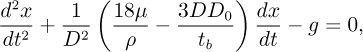
where ρ is the droplet density (much greater than that of air) and μ is the viscosity of the air. (Since D depends on t, this differential equation is fairly complicated, and its solution would most readily be obtained by a numerical method.)
If the droplet is always essentially at its terminal velocity, prove that the distance L it will fall before complete combustion is given by:

23. Particle ejection from fluidized bed—M (C). Fig. P4.23 shows a particle of mass M that is ejected vertically upward from the surface of a fluidized bed with an initial velocity υs. The velocity of the fluidizing gas above the bed is υg, and the resulting drag force on the particle is D = c(υg – v), where c is a constant and υ is the current velocity of the particle.

Prove that the maximum height h to which the particle can be entrained above the bed is given by:
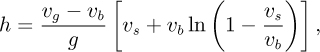
in which υb is the steady upward velocity of the particle when the drag and gravitational forces are balanced. Hint: You can take either of two approaches to develop the necessary differential equation in υ and z:
(a) Perform a conventional momentum balance and then involve the identity υ = dz/dt.
(b) Realize that a differential decrease in the kinetic energy of the particle equals the work done by the downward forces on the particle as it travels through a differential distance dz.
24. Plate-and-frame and rotary vacuum filters—D (C). Filtrate production from a compressible sludge is maintained by using both a plate-and-frame filter and a continuously operating rotary vacuum filter. The plate-and-frame filter produces 50 gpm of filtrate averaged over a day, using a slurry pump with a capacity of 100 gpm fitted with a relief valve to insure that the pressure does not exceed 60 psig. The time needed to clean the filter is 25 min.
The rotary vacuum filter has a diameter of 5 ft and a width of 5 ft, and the internal segments are arranged so that 20% of the total filtering surface is effective at any time. The filter drum rotates at half a revolution each minute, and the filtrate is produced at 25 gpm when the pressure inside the drum equals 8.2 psia, and at 30 gpm when the drum pressure is reduced to 3.2 psia. The slurry trough is at atmospheric pressure.
What is the minimum surface area required for the plate-and-frame filter? Assume that the rate of filtration is given by:
where V is the amount of filtrate produced per unit area of filter in time t, Δp is the pressure difference across the filter, and c and n are constants.
25. Pressure in a centrifugal filter—D. Consider the filter shown in Fig. 4.20, with the notation and equations given there. By starting from Eqns. (4.41), prove that the pressure in the cake and slurry are given in dimensionless form by:

Here, ![]() , R = r/r2, and subscripts 1 and a correspond to radii of r1 and a, respectively.
, R = r/r2, and subscripts 1 and a correspond to radii of r1 and a, respectively.
For a filter operating at Ra = 0.8, plot P versus R on a single graph for R1 = 0.7, 0.75, 0.78, and 0.8. Comment on your findings.
26. Transient effects in a centrifugal filter—D. Consider the centrifugal filter shown in Fig. 4.20, with the notation and equations given there.
If the flow rate of filtrate is steady and there is initially no cake, prove that after a time t the inner radius of the slurry is given by:

Hint: Start by using the relations for dp/dr in Eqn. (4.41) to obtain two expressions for the pressure pa at the slurry/cake interface; then eliminate pa and obtain an expression for r1.
A centrifugal filter operates with the following values: r2 = 0.5 m, ρ = 1,000 kg/m3, ω = 40π rad/s, κ = 3.2 × 10⁻¹³ m2, H = 0.5 m, Q = 0.005 m3/s, ε = 0.1, and μ = 0.001 kg/m s. After five minutes, what are the values of r1 and a?
27. Porous medium flow—D (C). Fig. P4.27 shows an apparatus for studying flow in a porous medium. Fluid of high viscosity μ flows between two parallel plates PP under the influence of a uniform pressure gradient dp/dx. Midway between the plates is a slab S of porous material of void fraction ε and permeability κ. The diagram shows the velocity profile in the fluid, the velocity within the slab being the interstitial velocity:
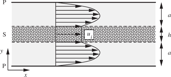
Explain why the velocity profile is of the form indicated, with particular attention to the boundary conditions at the slab surfaces. Show that the total flow rate Q per unit width is:

28. Plate-and-frame filtration—M (C). Derive the general filtration equation for a constant-rate period followed by a constant-pressure period:

where t is the total filtration time, tr is the time of filtration at constant rate, V is the total filtrate volume, Vr is the filtrate volume collected in the constant-rate period, A is the total cross-sectional area of the filtration path, r is the specific resistance of the filter cake, c is the resistance coefficient of the filter cloth, Vc is the volume of filter cake formed per unit volume of filtrate collected, and Δp is the pressure drop across the filter.
A plate-and-frame filter is to be designed to filter 300 m3 of slurry in each cycle of operation. A test on a small filter of area 0.1 m2 at a pressure drop of 1 bar gave the following results:
Assuming negligible filter-cloth resistance, estimate the filtration area required in the full-scale filter when the cycle of operation consists of half an hour at a constant rate of 2 × 10⁻³ m3/s m2, followed by one hour at the pressure attained at the end of the constant-rate period. Also evaluate this pressure.
29. Centrifugal pump efficiency—M (C). A single-stage centrifugal pump has swept-back vanes, which at the outlet make an angle β with the tangent to the outer diameter, whose value is D. The axial width at the outer periphery is b, and the rotational speed is N revolutions per unit time. There is no recovery of kinetic energy in the volute chamber, and the actual whirl velocity is the ideal value. Assuming the flow to be radial at the entry, show that the output head is:

in which u = πDN and f is the radial velocity of flow at the exit. Derive an expression for the power input, and show that the maximum efficiency is 1/(1 + sin β).
30. Distillation column flooding—E. Following the notation of Section 4.7, a bubble-cap distillation column has values H = 1 ft, CD = 0.62, D = 0.1 ft, W = 2 ft, and δ = 0.1 ft. If flooding is just to be avoided, what is the maximum liquid flow rate L (ft3/s) that can be accommodated? What are then the liquid velocity through the opening at the bottom of a downcomer and the height of the liquid above the weir?
31. Cyclone separator performance—E. Following the notation of Section 4.8, a cyclone separator has values A = 0.2 ft2, H = 2 ft, Q = 5 ft3/s, μ = 0.034 lbm/ft hr, and ρp = 120 lbm/ft3. What is the diameter of the smallest spherical particle that can be separated by the cyclone? Express your answer in both feet and microns (μm).
32. How fast did that dinosaur go?—M. Chemical engineers are often expected to be versatile, as in this problem, suggested by an article in the April 1991 issue of Scientific American, “How Dinosaurs Ran,” by R. McNeill Alexander. Assume that the speed u of a walking, running, or galloping animal depends on its leg length ℓ, its stride length s, and g (this because such locomotion involves some up-and-down motion). Perform standard dimensional analysis to show that the ratio s/l should be a function of the Froude number u2/gl.
Based on observations of different quadrupeds from cats to rhinoceroses, and two species of bipeds (humans and kangaroos), the article showed that with some experimental scatter, ln(s/l) ![]() 0.618 + 0.308 ln(Fr) + 0.035 [ln(Fr)]2.11 For most animals, the leg length is approximately four times the foot length or diameter.
0.618 + 0.308 ln(Fr) + 0.035 [ln(Fr)]2.11 For most animals, the leg length is approximately four times the foot length or diameter.
11 The article also showed a transition from a trotting to a galloping gait at Fr = 2.55, equally true whether the animal was a ferret or a rhinoceros!
Fossilized dinosaur tracks in a Texan gully showed footprints with an approximate diameter of 0.95 m and a stride length of 4.5 m. What was the speed of the dinosaur on that day?
33. Pressure drop in spherical reactor—M. Fig. P4.33 shows a spherical reactor of internal diameter D that is packed to a height H (symmetrically disposed about the “equator”) with spherical catalyst particles of diameter d and void fraction ε. A volumetric flow rate Q of a liquid of density ρ and viscosity μ flows through the packing.

How would you determine the resulting pressure drop? Give sufficient detail so that somebody else could perform all necessary calculations based on your plan.
34. Pumping into a filter—E. Fig. P4.34 shows a centrifugal pump with pressure increase p2 – p1 = a – bQ2 atm, where a and b are known constants, pumping a slurry into a plate-and-frame filter. The filter has a cross-sectional area A cm2, cake permeability κ darcies [(cm/s) cP/(atm/cm)], filtrate viscosity μ cP, and cake-to-filtrate volumetric ratio ε. A total volume V cm3 of filtrate has been passed. The pump inlet and filter exit pressures are equal.

If a = 0.2, b = 10–5, A = 100, κ = 100, μ = 1, ε = 0.1, and V = 104, all in units consistent with the above definitions, calculate the current volumetric flow rate Q cm3/s. Ignore the slight difference between slurry and filtrate volumes.
35. Equipment encyclopedia—M. Examine the Material Balances & Visual Equipment Encyclopedia of Chemical Engineering Equipment CD, discussed in Section 4.1, to answer the following ten questions:
(a) In the animation of the plate distillation column, how many trays are there?
(b) Above what value of the diameter is the plate distillation column the most cost efficient?
(c) What is the fluid medium in a hydrocyclone?
(d) In a cyclone, does the overflow contain the smaller or the larger particles?
(e) In a filter, what is the maximum ratio of volume of wash liquid to filtrate volume?
(f) In a rotary vacuum filter, approximately what fraction of the drum is submersed in the slurry?
(g) How many shapes of collectors can be used in electrostatic precipitators?
(h) In a packed-bed reactor, what is the two-word phrase for the variation of product concentration in the reactor?
(i) In the centrifugal pump section, how many head/flow rate curves are shown on a single graph?
(j) In a fluidized-bed reactor, what is the typical range in size of the catalyst particles?
36. Approximation for falling sphere—M. Referring to Example 4.2, prove for small times that Eqn. (E4.2.7) can be approximated by Eqn. (E4.2.8).
37. True/false. Check true or false, as appropriate:
(a) In a centrifugal pump, the major portion of the pressure increase occurs as the fluid passes through the vanes of the impeller.
T ![]() F
F ![]()
(b) For most designs of centrifugal pumps, the head increases as the flow rate increases because of the greater kinetic energy.
T ![]() F
F ![]()
(c) Data for centrifugal pumps of a given design may be correlated by plotting Δp/(ρD2N2) against Q/(ND3).
T ![]() F
F ![]()
(d) If two centrifugal pumps are placed in parallel, the overall pressure increase for a given total flow rate Q will be twice what it is for a single pump with the same flow rate Q.
T ![]() F
F ![]()
(e) Rotational speed N is related to the angular velocity of rotation ω by the equation N = 2πω.
T ![]() F
F ![]()
(f) The drag coefficient is a dimensionless force per unit area.
T ![]() F
F ![]()
(g) Flow around a sphere is laminar for a Reynolds number of 1,000.
T ![]() F
F ![]()
(h) Stokes’ law for the drag force on a sphere is F = 3πμu∞D.
T ![]() F
F ![]()
(i) For flow around a sphere, there is a transition region from laminar to turbulent flow in which the value of the drag coefficient is quite uncertain.
T ![]() F
F ![]()
(j) Consider a sphere settling at its terminal velocity in a fluid. If the following dimensionless group is known to have the value of 10,000:
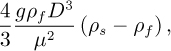
then the corresponding value of the drag coefficient is approximately 2.5.
T ![]() F
F ![]()
(k) When a descending sphere has reached its terminal velocity, Stokes’ law is always satisfied.
T ![]() F
F ![]()
(l) Analysis of the performance of a spray-drying column involves a knowledge of the drag on particles.
T ![]() F
F ![]()
(m) The sphericity of a cube is greater than that of a sphere of the same volume because the cube has more surface area.
T ![]() F
F ![]()
(n) Turbulent flow through a packed bed can be modeled as flow through a noncircular duct.
T ![]() F
F ![]()
(o) The Ergun equation applies for both laminar and turbulent flow.
T ![]() F
F ![]()
(p) The Burke-Plummer and Blake-Kozeny equations are limiting forms of the Ergun equation, for low and high values of the Reynolds number, respectively.
T ![]() F
F ![]()
(q) A tubular reactor is packed with catalyst particles, each of which is a cylinder of diameter 1 cm and length 2 cm. The effective particle diameter is 0.5 cm.
T ![]() F
F ![]()
(r) A high permeability means that a porous medium offers a high resistance to flow through it.
T ![]() F
F ![]()
(s) For flow through a porous material, the pressure drop is usually proportional to the square of the flow rate.
T ![]() F
F ![]()
(t) After a frictional dissipation term F has been established for flow in a packed bed, it may be used in an energy balance for flow in either horizontal, vertical, or inclined directions, provided the flow rate is not changed.
T ![]() F
F ![]()
(u) To convert from darcies to cm2, multiply by 1.06 ×10⁻¹¹ approximately.
T ![]() F
F ![]()
(v) In constant-pressure operation of a filter, the amount of filtrate passed is directly proportional to the elapsed time.
T ![]() F
F ![]()
(w) If a plate-and-frame filter is operated at a constant flow rate, the pressure drop across it is proportional to the square root of the elapsed time.
T ![]() F
F ![]()
(x) Fluidized particles behave essentially as though they were a liquid.
T ![]() F
F ![]()
(y) A person who can swim in water could probably also swim in a fluidized bed of sand particles, assuming the bed were large enough.
T ![]() F
F ![]()
(z) Dynamical similarity means that a scale model looks exactly like a full-size object (pump, ship, etc.), except only for differences in size.
T ![]() F
F ![]()
(A) Geometrical similarity means that a scale model (of a pump, ship, etc.) has exactly the same values of the dimensionless groups (Reynolds number, for example) as the corresponding full-size object.
T ![]() F
F ![]()
(B) A friction factor is essentially a ratio of shear forces to viscous forces.
T ![]() F
F ![]()
(C) The Stokes number is essentially a ratio of gravitational forces to inertial forces.
T ![]() F
F ![]()
(D) The Grashof, Nusselt, Peclet, and Prandtl numbers are related to heat transfer.
T ![]() F
F ![]()
(E) The Froude number is a measure of the ratio of inertial forces to gravitational forces.
T ![]() F
F ![]()
(F) The Froude number is important in determining the drag on ships because it represents the ratio of viscous forces to gravitational forces.
T ![]() F
F ![]()
(G) A plate-and-frame filter has the disadvantage that it is subject to intermittent operation.
T ![]() F
F ![]()
(H) For constant-pressure operation of a plate-and-frame filter, the volume of filtrate is proportional to the elapsed time.
T ![]() F
F ![]()
(I) Progressing radially outward in a centrifugal filter, the pressure typically increases in the slurry and decreases in the cake.
T ![]() F
F ![]()
(J) There is a definite upper limit on the liquid throughput that a bubble-cap distillation column can handle.
T ![]() F
F ![]()
(K) Between the gas inlet and exit in a cyclone, a forced vortex exists, in which the tangential velocity υθ is proportional to the radial distance from the centerline.
T ![]() F
F ![]()
(L) A cyclone can separate particles from a gas more easily at low flow rates.
T ![]() F
F ![]()