
Chapter 8. Boundary-Layer and Other Nearly Unidirectional Flows
8.1. Introduction
Although the Navier-Stokes equations apply to the flow of a Newtonian fluid, they are—in general—very difficult to solve exactly. There is also the problem that an apparently correct solution may be physically unrealistic for high Reynolds numbers, because of turbulence or other instabilities.
Two particular types of simplifying approximations may be made, depending on the Reynolds number (the ratio of inertial to viscous effects), in order to make the situation more tractable:
1. Omit the inertial terms, as was done in the examples of Chapter 6. The resulting equations are typically appropriate for the flow near a fixed boundary, where viscous action is particularly important. (Another example, not given there, leads to the Stokes’ solution for “creeping” flow round a sphere, but is valid only for Re < 1.)
2. Omit the viscous terms, as was done in Chapter 7. The resulting equations for inviscid flow are often fairly easy to handle, and are frequently adequate for applications away from boundaries, where viscous action is relatively unimportant.
Generally, however, there will be a region in which both viscous and inertial terms are of comparable magnitude; even for a low-viscosity fluid, such a region will occur near a solid boundary, where there is a high shear rate. These regions are called boundary layers, and are important in some chemical engineering operations because diffusion of heat or mass across them frequently controls the rate of some heat- and mass-transfer operations. Also, in aerospace engineering and naval architecture, a knowledge of boundary-layer theory is essential for determining the drag on airplane bodies and wings and on ship hulls.
A key feature of boundary-layer analysis is the existence of a primary flow direction, whose velocity component υx is considerably larger than that in a trans-verse or secondary direction, such as υy. The fact that υx ≫ υy typically implies essentially no pressure variation in the transverse direction—a substantial simplification. The same simplification also applies to lubrication problems, polymer calendering, paint spreading, and other “nearly unidirectional” flows.
8.2. Simplified Treatment of Laminar Flow Past a Flat Plate
The full analytical solution of the Navier-Stokes equations for boundary-layer flow is virtually impossible, so that in Sections 8.2–8.5 we are content to make simplifications and still obtain realistic solutions by the following two approaches:
1. Perform mass and momentum balances on an element of the boundary layer, then assume a reasonable shape for the velocity profile, and finally solve by the method outlined in this section for laminar flow and in Section 8.5 for turbulent flow.
2. For laminar boundary layers only, perform the classical Blasius solution, starting with the Navier-Stokes equations and dropping those terms that are expected to be small (see Section 8.3). As discussed in Section 8.4, a suitable change of variables leads to a third-order ordinary differential equation, which can be solved numerically in order to obtain the velocities.
Additionally, in Examples 8.3 and 8.5, we show how computational fluid dynamics can solve the full Navier-Stokes equations for boundary-layer and lubrication flows.
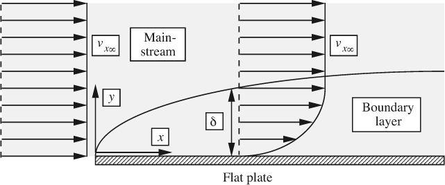
For the present, consider steady two-dimensional laminar flow past a flat plate, shown in Fig. 8.1, and assume the existence of a boundary layer, being a thin region in which the velocity changes from zero at the plate to practically its value υx∞ in the mainstream. The velocity υx∞ in the mainstream (where viscous effects are negligible) will be considered constant for the present; therefore, from Bernoulli’s equation, the pressure in the mainstream does not vary. Further, since there is likely to be a negligible pressure variation across the boundary layer (see Section 8.3 for a rigorous proof), the pressure in the boundary layer is also constant.
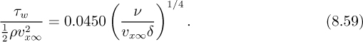
The almost exact Blasius solution, to be treated in Section 8.4, will show that the shear force τω exerted on the plate at any distance x from its leading edge is given in dimensionless form by the drag coefficient, cf, as:

In this section, we shall obtain a comparable result much more easily, by performing mass and momentum balances on an element of the boundary layer, as shown in Fig. 8.2.
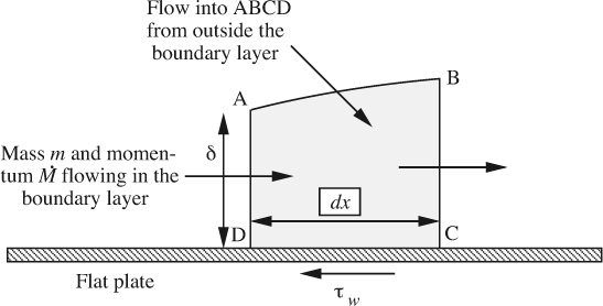
Let the length of the element be dx, and consider unit width normal to the plane of the diagram. The y velocity component υy arises because the plate retards the x velocity component; thus, ∂υx/∂x is negative, and—from continuity—∂υy/∂y must be positive; since υy is zero at the wall, it becomes increasingly positive away from the wall. By integration over the thickness of the boundary layer, the following total fluxes of mass (m) and momentum (![]() ) entering through the left-hand face AD are obtained1:
) entering through the left-hand face AD are obtained1:

1 There is no need for a dot over m, which has already been defined as the rate of transfer of mass, M.
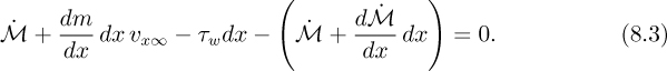
By the usual arguments, the mass flux leaving through the face BC will be m + (dm/dx)dx. That is, a mass flux of (dm/dx)dx must be entering from the mainstream across the interface AB into the control volume ABCD. Since its velocity is υx∞, it will be bringing in with it an x-momentum flux of (dm/dx)dx υx∞. A momentum balance on ABCD in the x direction yields:
Note that both inertial and viscous terms (the latter via the wall shear stress τω) are involved, consistent with the definition of a boundary layer expressed in Section
8.1. There are no terms involving pressure, since this is constant everywhere. Substitution of m and ![]() from Eqn. (8.2), and division by ρ, gives:
from Eqn. (8.2), and division by ρ, gives:

Equation (8.4) will enable the wall shear stress and the boundary-layer thickness to be predicted as a function of x if the velocity distribution υx = υx(x, y) is known.
The simplified approach pursued here assumes that the velocity profile obeys the law:
Equation (8.5) is assumed to hold at all distances x from the leading edge, even though the boundary-layer thickness δ depends on x; that is, the velocity profiles have similar shapes, but are “stretched” more in the y direction the further the distance from the leading edge, as shown in Fig. 8.3. Note that ζ is a dimensionless distance normal to the plate. The principle employed is that of “similarity of velocity profiles”; that is, at a particular distance from the plate—expressed as a fraction of the local boundary-layer thickness—the velocity will have built up to a certain fraction of the mainstream velocity, independent of the distance x from the leading edge.

The next step is to make a reasonable speculation about the form of f(ζ), which should conform to the following conditions at least:
1. f(0) = 0 (zero velocity at the wall, where ζ = 0).
2. f(1) = 1 (the mainstream velocity υx∞ is regained at the edge of the boundary layer, where ζ = 1).
3. f ′(1) = 0 (the velocity profile has zero slope at the junction between the boundary layer and the mainstream).
If required, higher-order derivatives can be obtained at y = 0 and y = δ by successive differentiations of the simplified x momentum balance (see Section 8.3 for details):
For example,


The present choice will be:
which not only conforms to conditions 1, 2, and 3 above, but also yields the indicated values for the following integrals:

Differentiation of both Eqns. (8.10) with respect to x, followed by multiplication by υ2x∞, gives:

which can then be substituted into the momentum balance of Eqn. (8.4):
Equation (8.12) is an ordinary differential equation governing variations in the boundary-layer thickness with distance from the leading edge, and which can be integrated as soon as the wall shear stress is known. Differentiation of the velocity profile of Eqn. (8.9) leads to:

Equation (8.12) then becomes:
Separation of variables and integration gives:
That is, the thickness of the boundary layer varies with distance from the leading edge as:
The wall shear stress can now be obtained from Eqns. (8.13) and (8.16). After some algebra, there results:
In view of the highly simplified approach taken, this last result compares very favorably with the Blasius solution of Section 8.4.
Of course, other approximations can be made for the velocity profile, such as υx/υx∞ = aζ + bζ2 + cζ3+.... Similar results follow, and Table 8.1 indicates the corresponding numerical coefficients that will appear in Eqn. (8.17).

Example 8.1—Flow in an Air Intake (C)
The device shown in Fig. E8.1 is used for measuring the flow of air of density ρ into the circular intake port of an engine. Basically, it uses Bernoulli’s equation between two points: (a) far upstream of the intake, where the velocity is essentially zero and the pressure is p1, and (b) the pressure tapping at a distance x from the inlet, where the pressure is measured to be p2.
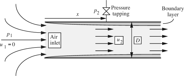
The situation is complicated by the formation of a boundary layer as the air impinges against the inlet of the port, so the velocity profile at the location of the tapping consists of: (a) a central core, in which the velocity is uniformly u2, and (b) a boundary layer in which the velocity declines from its mainstream value υx∞ = u2 to zero at the wall.
Bernoulli’s equation can be applied, starting from the outside air (where u1 ![]() 0) and continuing into the core (where viscosity is negligible), leading to:
0) and continuing into the core (where viscosity is negligible), leading to:

However, the ultimate goal is to be able to determine the mean velocity um (defined as the total flow rate divided by the total area), which necessitates the introduction of a discharge coefficient CD, so that:
The total mass flow rate of air is then:
where A is the cross-sectional area of the pipe, which has an internal diameter D.
If D = 2 in., x = 1 ft, ν = 1.59 × 10⁻⁴ ft2/s, and um = 20 ft/s, estimate CD.
First, estimate the properties of the boundary layer. The largest value of the Reynolds number occurs opposite the pressure tapping, where x = 1 ft. Also, a rough estimate of the mainstream velocity is um, so that υx∞ ![]() 20 ft/s. Thus, to a first approximation:
20 ft/s. Thus, to a first approximation:
From Section 8.5, the flow in the boundary layer is therefore laminar all the way from the inlet to the pressure tapping, and the result of Eqn. (8.16), which was based on the assumed velocity profile υx/υx∞ = sin(πy/2δ), applies:

giving a first approximation of the thickness of the boundary layer:
Thus, the boundary layer has an outer diameter of 2.000 in. and an inner diameter of (2.000 –2 × 0.162) = 1.676 in., for a mean diameter of Dm =(2.000+1.676)/2 = 1.838 in.
Although the intake has circular geometry, the boundary layer can be approximated as that on a flat plate of width πDm. The corresponding mass flow rate in the boundary layer is:

The total mass flow rate, which is based on the mean velocity, equals the sum of the mass flow rates in the core and in the boundary layer:
which gives the improved estimate υx∞ ![]() 22.4 ft/s. The calculations can be repeated iteratively; convergence essentially occurs after just one more iteration, giving a final value υx∞
22.4 ft/s. The calculations can be repeated iteratively; convergence essentially occurs after just one more iteration, giving a final value υx∞ ![]() 22.29 ft/s. Since the pressure drop based on Bernoulli’s equation gives υx∞
22.29 ft/s. Since the pressure drop based on Bernoulli’s equation gives υx∞ ![]() 22.29, and the actual mean velocity is a lower value, um = 20.0, the required discharge coefficient is:
22.29, and the actual mean velocity is a lower value, um = 20.0, the required discharge coefficient is:
8.3. Simplification of the Equations of Motion
Here, we start with the Navier-Stokes and continuity equations, and inquire as to which terms are likely to be insignificant, so that they may be dropped and the equations thereby simplified. In two dimensions, assuming steady flow and the absence of gravitational effects, the starting equations are:


Now investigate the relative orders of magnitude of the various terms in Eqns. (8.18), (8.19), and (8.20). Let “O” denote “order of”; for example υx = O(υx∞), because for much of the boundary layer, the x velocity component υx is a significant fraction (0.1 or more, for example) of the mainstream velocity υx∞; nowhere is υx larger than υx∞. Also, make the following two key (and realistic) assumptions at any location x:
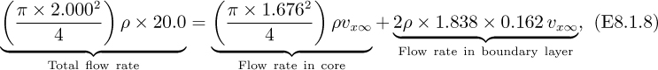
1. The derivative ∂υx/∂x is of the same order of magnitude as the corresponding mean gradient from the origin to x. The situation is illustrated in Fig. 8.4(a), which shows for a given y how υx declines from υx∞ at the leading edge (x = 0) to a much smaller value for significant values of x. The magnitude of the slope of the chord, which represents the mean velocity gradient, is approximately υx∞/x, and the diagram shows that the slope of the velocity profile at two representative points is not vastly different from υx∞/x. That is, ∂υx/∂x = O(υx∞/x).
Fig. 8.4 Illustration of orders of magnitude: (a) for ∂υx/∂x, with two representative intermediate tangents, and (b) for ∂υx/∂y. Note that the slope is much higher in (b) than in (a), because υx changes from zero to υx∞ over a very short distance, δ.
2. The velocity gradient of υx in the y direction is of the same order as the corresponding mean gradient from y = 0 to y = δ. The situation is illustrated in Fig. 8.4(b), which shows for a given x how υx increases from zero at the wall (y = 0) to υx∞ at the edge of the boundary layer (y = δ). The magnitude of the slope of the chord, which represents the mean velocity gradient, is approximately υx∞/δ. Further reflection shows that the slope of the velocity profile at a few representative locations between the wall and the edge of the boundary layer is nowhere vastly different from υx∞/δ. That is, ∂υx/∂y = O(υx∞/δ). Because δ is much smaller than x, the slope in Fig. 8.4(b) is much greater than that in Fig. 8.4(a), and representative intermediate slopes cannot be drawn clearly.
Orders of magnitude of individual derivatives. Based on the above two assumptions, and by following similar arguments and also invoking the continuity equation in Eqn. (8.20), we obtain the following orders of magnitude:

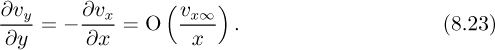
Since υy = 0 at y = 0, Eqn. (8.23) leads to:

The various derivatives of υy therefore have the following orders of magnitude:

Examination of the x momentum balance. Based on the above, all of the terms in Eqn. (8.18), except the pressure gradient, may be assigned their appropriate orders of magnitude:
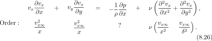
By hypothesis, the thickness of the boundary layer is much less than the distance from the leading edge. Hence, δ ≪ x, and on the right-hand side of Eqn. (8.26) the second-order derivative of υx with respect to x is negligible compared to the derivative with respect to y. Also, because inertial and viscous terms are both important in the boundary layer, their orders of magnitude can be equated, giving:

Hence, since δ ≪ x, Rex = υx∞x/ν must be large, which excludes the analysis from applying very close to the leading edge. Also note that:

This last equation gives the order of the pressure gradient ∂p/∂x if it is important; however, in certain cases—notably when the mainstream velocity is constant—this pressure gradient may be zero.
Examination of the y momentum balance. Similar considerations apply to the terms in Eqn. (8.19), except for the pressure gradient, whose order of magnitude is again unknown: Order:
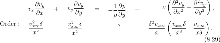
Note that the ∂2υy/∂x2 term is of a lower order than the others and can be neglected. It therefore follows that:
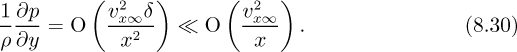
That is, the variation of pressure p across the boundary layer in the y direction is small in comparison to that in the x direction [see Eqn. (8.28)], so that p is (at most) a function of x only:
The simplified equations of motion are therefore:

Pressure variation in the mainstream. In the mainstream, where by hypothesis the effect of viscosity is negligible:
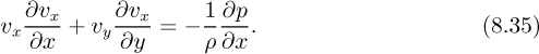
Thus, if appreciable velocity gradients exist in the mainstream, it follows that (∂p/∂x)/ρ is of the same order as υx(∂υx/∂x), namely ![]() , and must therefore be retained in the x momentum balance, Eqn. (8.18). An alternative viewpoint in the mainstream, which is removed from the plate and hence has negligible viscous effects, is to apply Bernoulli’s equation and then differentiate it:
, and must therefore be retained in the x momentum balance, Eqn. (8.18). An alternative viewpoint in the mainstream, which is removed from the plate and hence has negligible viscous effects, is to apply Bernoulli’s equation and then differentiate it:

which is the same result as obtained from Eqn. (8.35) if the term involving υy is neglected.
8.4. Blasius Solution for Boundary-Layer Flow
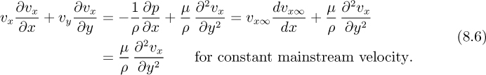
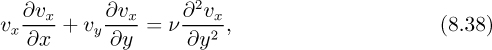
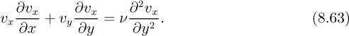
In Section 8.3, by considering the relative magnitudes of the various derivatives, we had greatly simplified the equations of motion. If the additional assumption is made that the mainstream velocity is constant, the pressure is also everywhere constant, leaving only the simplified x momentum balance and the continuity equation for consideration:
In addition, the boundary conditions are that both velocity components are zero at the plate, and that the mainstream velocity is attained well away from the plate:
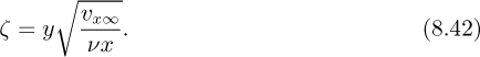
The key to the solution of this simplified problem is to introduce a new space variable, ζ, which combines both x and y, and is motivated by observing that the simplified integral momentum balance led to δ being proportional to ![]() :
:
Also introduce a stream function (see also Section 7.3) ψ, such that:
which automatically satisfies the continuity equation, (8.39). Also try a separation of variables of the form:
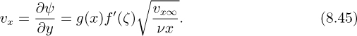
Next, try to make υx/υx∞ a function of ζ only, by choosing:
which gives:


Substitution of υx and υy and the derivatives of υx from Eqns. (8.47) and (8.48) into Eqn. (8.38) leads to the following ordinary differential equation:
subject to the boundary conditions:
The original Blasius solution divided ζ = 0 to ∞ into two regions and obtained approximate solutions (involving an infinite series and a double integral) for each such region. Three arbitrary constants appeared in the solution, and these were evaluated by requiring continuity of f, f ′, and f ″ at the junction between the two regions.
With computer software readily available for solving simultaneous ordinary differential equations, we have opted for a numerical solution of Eqns. (8.49)– (8.51), first giving f as a function of ζ, and then the velocity components from Eqns. (8.47) and (8.48). The values shown in Fig. 8.5 agree completely with the original Blasius solution. The reader who wishes to check these results can do so fairly readily (see Problem 8.14).2
2 The values shown in Fig. 8.5 were computed by a numerical solution of Eqn. (8.49), by B. Carnahan, H.A. Luther, and J.O. Wilkes, as shown on page 414 of their book, Applied Numerical Methods, Wiley & Sons, New York, 1969.

As a by-product, the solution yields the following value for the second derivative of f at the wall:
which then enables the wall shear stress to be deduced:

The drag coefficient, which is a dimensionless shear stress, is then:
Experiments of Nikuradse (Rex from 1.08 × 10⁵ to 7.28 × 10⁵) verify the predicted velocity profile. There is a transition from laminar into turbulent flow at higher Reynolds numbers.
8.5. Turbulent Boundary Layers
The preceding analysis in Sections 8.2–8.4 was for laminar flow in the boundary layer. However, it is found experimentally that the boundary layer on a flat plate becomes turbulent if the Reynolds number, Rex, exceeds approximately 3.2 × 10⁵, which is next investigated. Assume for simplicity that the flow is everywhere turbulent—from the leading edge of the plate (x = 0) onward. In reality, the boundary layer will be laminar in the vicinity of the leading edge and would, for large enough x, undergo a transition to turbulent flow; thus, if the accuracy of the situation warranted it, the separate portions of the layer (laminar and turbulent) could be analyzed individually and then combined.
The analysis begins exactly as previously, in which a momentum balance on an element of the boundary layer leads to Eqn. (8.4):

From experience with turbulent velocity profiles in pipe flow, assume (reasonably) that the one-seventh power law holds for the time-averaged x velocity in the turbulent boundary layer:
This last relation will be adequate for substitution into the two integrals of Eqn. (8.55) but it cannot be used for obtaining the shear stress at the wall—as was done previously in Eqn. (8.13)—since it predicts an infinite velocity gradient at the wall (y = 0).
For the shear stress we again have to draw an analogy with the shear stress for turbulent pipe flow. Recall the Blasius equation, (3.40), which is based on experiment and holds for smooth pipe up to a Reynolds number of about 105:
which, by substituting for the mean velocity υm in terms of the centerline or maximum velocity υmax, may be rephrased as:
where ν is the kinematic viscosity and a is the pipe radius. Therefore, for the wall shear stress for the boundary-layer case, assume essentially the same law, namely:
From Eqns. (8.55), (8.56), and (8.59), there results:

which, upon integration, gives:

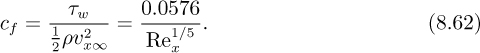
with a corresponding local skin friction coefficient of:
Example 8.2—Laminar and Turbulent Boundary Layers Compared
Compare the relative thicknesses and drag coefficients of laminar and turbulent boundary layers at the transition Reynolds number, Rex = 3.2 × 10⁵.
Solution
1. Thicknesses. The relevant equations for the ratio δ/x and their values at the indicated Reynolds number are:

so that the turbulent boundary layer is about 3.52 times thicker than the laminar boundary layer at the transition.
2. Drag coefficient. The relevant equations for cf and their values at the indicated Reynolds number are:

so that the turbulent boundary layer has a drag coefficient about 3.93 times that of the laminar boundary layer at the transition.
However, note that turbulence in the wake of a nonstreamlined object (see Section 8.7) can postpone separation of the boundary layer and lead to a reduced drag.
8.6. Dimensional Analysis of the Boundary-Layer Problem
Much information relating to the Blasius solution can be obtained by an intriguing dimensional analysis of the governing differential equations and boundary conditions.3 From Eqns. (8.38) and (8.39):
3 A good summary of the approach is given by J.D. Hellums and S.W. Churchill, “Simplification of the mathematical description of boundary and initial value problems,” American Institute of Chemical Engineers Journal, Vol. 10, No. 1, pp. 110–114 (1964).
x Momentum:
Continuity:
Boundary conditions:
First, introduce dimensionless coordinates and velocities as follows:
Here, xr and yr are reference distances, and υxr and υyr are reference velocities. At this stage it is important not to equate xr and yr, nor υxr and υyr, as this may limit our options by being too restrictive. Note that we also resist for the present the temptation to equate either υxr or υyr to the mainstream velocity, υx∞.
In terms of the dimensionless variables, the governing equations become:
x Momentum:

Continuity:
Boundary conditions:
Since these equations completely specify the problem, the dependent variables U and V must be functions of the independent variables X and Y and of the dimensionless groups that appear in the equations:


Here, f and g are two functions, unknown as yet.
Since the reference quantities are arbitrary, we may equate each dimensionless group to a constant, taken as unity for simplicity:
Equation (8.74) gives the following expressions for the three reference quantities υxr, yr, and υyr, in terms of the fourth reference quantity, xr:

The functional relationship for the x-velocity component now becomes:

Since xr did not appear in the problem statement, it must disappear from Eqn. (8.76). Hence, f must be some function of the first group divided by the square of the second group, resulting in:

Strictly speaking, the second function in Eqn. (8.77) should be distinguished from the first, but since both of them are unknown, we have used the common designation of “f.” In proceeding from Eqn. (8.76) to (8.77), it looks as though we have merely set xr = x, but this is not the case.
Similarly, the functional relationship for the y velocity component is:


Again, since xr did not appear in the problem definition, it must cancel out from both sides of Eqn. (8.79), whose form is therefore:

so that:

Note the following important points from the above development:
1. Equations (8.77) and (8.81) indicate how experimental data may be correlated most economically—that is, by constructing plots of:

2. The reference distances and velocities were not the same, leading to a more precise result than if we had insisted on xr = yr = ν/υx∞ and υxr = υyr = υx∞ at the outset.
3. The analysis clearly suggests the introduction of a new space variable,
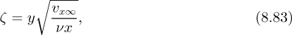
and indeed this was employed in Blasius’s solution.
The expression for the wall shear stress is:

which gives, in dimensionless form:

Observe that apart from the single unknown coefficient c, dimensional analysis has predicted a form that is in complete agreement with Eqn. (8.54) from the Blasius solution. In principle, a single precise experiment then gives the solution, c ![]() 0.332.
0.332.
8.7. Boundary-Layer Separation
Previous sections have discussed both laminar and turbulent boundary layers on a flat plate, in which there was a constant mainstream velocity and hence a constant pressure. Now consider Eqn. (8.32) applied close to the wall, where both υx and υy are small, so that:
Since ∂p/∂x = 0, the second derivative of the velocity is also zero, so the velocity gradient ∂υx/∂y is a constant near the wall, as in Fig. 8.6(a).
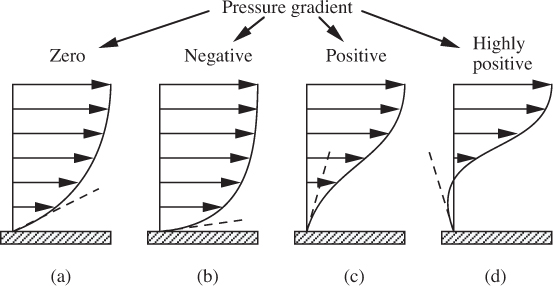
For more complex situations, the flow in the mainstream may not be uniform, leading to the following possibilities:
(a) A negative pressure gradient, ∂p/∂x < 0, in which case the velocity gradient near the wall decreases as we proceed out from the wall. Since the velocity must match the mainstream value at the edge of the boundary layer, this implies that the velocity gradient is steeper at the wall, as in Fig. 8.6(b).
(b) A positive pressure gradient, ∂p/∂x > 0, in which case the velocity gradient near the wall increases as we proceed out from the wall. Since the velocity must match the mainstream value at the edge of the boundary layer, this implies that the velocity gradient is less steep at the wall, as in Fig. 8.6(c). In a more extreme case, in which ∂p/∂x is more highly positive, the gradient can actually become zero (or even slightly negative) at the wall, as in Fig. 8.6(d).
The modification of the velocity profile by the pressure gradient is similar to that shown in Fig. 8.11 for the flow of lubricant in a bearing.
Consider now the flow past an object that is not particularly well streamlined, such as the sphere shown in Fig. 8.7(a). On the upstream hemisphere, the streamlines are pushed closer together, so in the direction of flow the velocity increases and the pressure decreases—a relatively stable situation. On the downstream hemisphere, the opposite occurs, and the pressure increases in the direction of flow, leading to the situations shown in Fig. 8.6(c) and (d).

Under such circumstances, the boundary layer no longer “hugs” the surface but separates from it, leading to considerable turbulence and loss of pressure in the wake of the sphere, causing a substantial increase in the drag. It is clearly desirable in most cases to delay the onset of separation, and indeed this can be done and often totally prevented for flow past a well streamlined surface such as an airplane wing. Boundary-layer separation was first examined extensively by Ludwig Prandtl.
Another way of delaying the separation is somewhat paradoxical—to make sure that the boundary layer is turbulent, which can often be achieved by roughening part or all of the surface, as in the dimples on a golf ball.4 Under these turbulent circumstances, momentum in the form of velocity is transmitted much more rapidly from the mainstream to the boundary layer, thus helping to insure that the velocity near the boundary does not stagnate, but continues with a positive value. The onset of separation is therefore postponed, as in Fig. 8.7(b).
4 Do you know how many dimples there are on a golf ball? According to Ian Stewart in “Mathematical Recreations” on page 96 of Scientific American, February 1997, considerations of symmetry dictate that the most frequently occurring numbers of dimples are 252, 286, 332, 336, 360, 384, 392, 410, 416, 420, 422, 432, 440, 480, 492, and 500.
The sudden “dip” in the drag coefficient for a sphere at a high Reynolds number, as in Fig. 4.7, can now be explained. It is because the flow in the boundary layer has become turbulent and the previous high degree of separation of the laminar boundary layer no longer exists. Such events—in conjunction with spin and seam orientation—are also important in determining the trajectory of a baseball.5
5 A.T. Bahill, D.G. Baldwin, and J. Venkateswaran, “Predicting a baseball’s path,” Scientific American, pp. 218–225 (May/June 2005).
Example 8.3—Boundary-Layer Flow Between Parallel Plates (COMSOL Library)
A fluid of density 1,000 and viscosity 0.01 flows freely in the y direction with an initially uniform velocity υ0 = 0.02. After a distance of y = 0.01 it encounters flat plates of length 0.04 located at x = ±0.01. The exit pressure from the plates is p = 0. The corresponding boundary conditions are shown in Fig. E8.3.1. All units are mutually consistent.
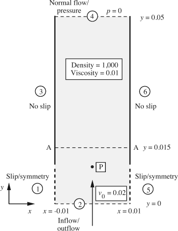
A. Initial check. This problem is entitled “Parallel Plates” in the COMSOL library. Open it, and first check:
1. The values for the viscosity and the density.
2. The six boundary conditions.
B. Overall plots. Print the following plots for the whole region in Fig. E8.3.1:
3. The streamlines.
4. Arrows showing the velocity vectors.
5. A two-dimensional contour plot of the velocity.
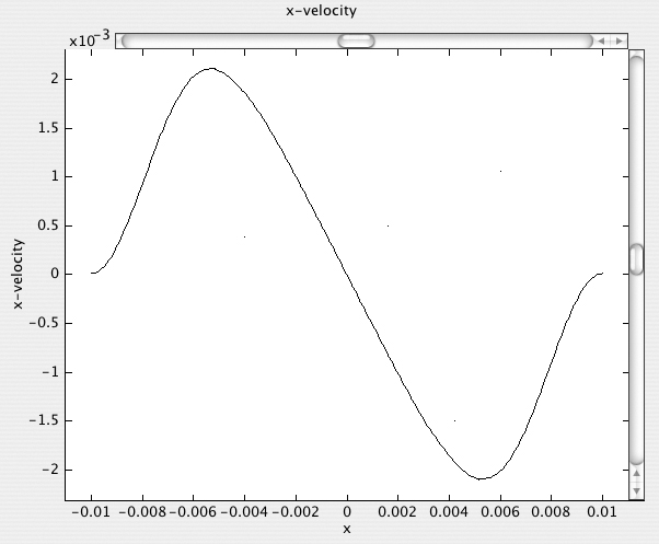
C. Cross-section plots. For y = 0.015, plot and print the following at section A–A between the two plates, and comment briefly on each:
7. The x velocity.
8. The vorticity.
D. Values at point P. Finally, comment on the relative values of the pressure and y velocity υy at x = 0, y = 0.01, marked as P in Fig. E8.3.1., and at the exit (x = 0, y = 0.05).
Solution
A. Initial check. In COMSOL, choose the sequence Model Library, Chemical Engineering Module, Momentum Transport, and parallel plates, which will show the velocity field in color.
Start by selecting Constants under the Options pulldown menu, and observe that rho, eta, and v0 have been assigned the values 1,000, 0.01, and 0.02, respectively. Then choose Subdomain Settings under the Physics pulldown menu and highlight the solitary subdomain 1. The density and viscosity are clearly set to the constants rho and eta.
Likewise, choose Boundary Settings under the Physics pulldown menu and highlight each of the six boundary segments in turn. You will see that each segment corresponds to one the types indicated in Fig. E8.3.1, and that the corresponding boundary appears in red.
B. Overall plots. By selecting appropriate choices in Plot Parameters under Postprocessing (Streamline, Arrow, and Surface), the overall picture of the flow is displayed in Fig. E8.3.2. After the initial small “free-flow” entrance region, the formation of boundary layers on the two plates is very evident, either by examining the movement of the streamlines away from the plates or by noting the reduction in velocity adjacent to the plates. From continuity, this velocity reduction also causes an acceleration in the middle of the stream.

Fig. E8.3.2 Three overall views of the flow: (a) the upward moving streamlines, for which 40 streamline “start points” were specified under plot parameters; the horizontal line is the section A–A in Fig. E8.3.1 and appears automatically only after the cross-section plots have been done; (b) the velocity vectors; and (c) a two-dimensional plot (the original being in color) showing the velocities, the approximate magnitudes of which have been added.
C. Cross-section plots. The three requested plots at y = 0.015 are obtained by selecting Line/extrusion under Cross-Section Plot Parameters and entering x0 = -0.01, x1 = 0.01, y0 = 0.015, y1 = 0.015 in the Cross-section line data window, then asking in sequence under y-axis data for plots of the y velocity, x velocity, and vorticity. The results are shown in Figs. E8.3.3–E8.3.5, for which we make the following comments:
1. The velocity υy in the primary flow direction is still essentially flat in the central region, falling to zero as the wall is reached.
(a) At values of x that are clearly in the boundary layer, such as x = –0.008 and x = 0.008 in Fig. E8.3.3, υy would continue to decrease in the y direction, so that ∂υy/∂y is negative at these locations.
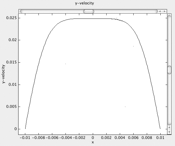
(b) In the central core υy continues to accelerate as seen in Fig. E8.3.2(c), so that the reverse occurs and ∂υy/∂y is positive.
2. Following on Item 1(a), the continuity equation, ∂υx/∂x + ∂υy/∂y = 0, mandates that ∂υx/∂x must be positive in the boundary layer, and this is evidenced in Fig. E8.3.4 at, for example, x = –0.008 and x = 0.008. Conversely, from Item 1(b), ∂υx/∂x must be negative in the central core, and this is also clearly seen.
3. The vorticity is ∂υy/∂x –∂υx/∂y ![]() ∂υy/∂x (because υy ≫ υx), leading to a positive vorticity (counterclockwise rotation) near the left-hand plate and a negative vorticity (clockwise rotation) near the right-hand plate. In the central region the vorticity is essentially zero because υy is virtually constant there.
∂υy/∂x (because υy ≫ υx), leading to a positive vorticity (counterclockwise rotation) near the left-hand plate and a negative vorticity (clockwise rotation) near the right-hand plate. In the central region the vorticity is essentially zero because υy is virtually constant there.
D. Values at point P. Finally, the pressure p and velocity υy at the entrance point P are obtained by first choosing the sequence Plot Parameters, Surface, and Predefined quantities, and then requesting pressure and y velocity plots. Then, clicking on the point (x = 0, y = 0.01) shows the values p = 0.334018 and υy = 0.022147 in the lower left-hand corner. Similarly, the exit centerline values are p = 0 (given) and υy = 0.029838. As expected at the centerline, there is an acceleration from P to the exit and a corresponding reduction in pressure.

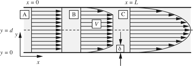
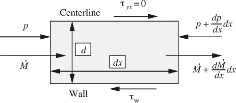
Example 8.4—Entrance Region for Laminar Flow Between Flat Plates
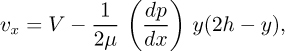
In Example 6.1, involving laminar flow between parallel plates, only the velocity in the axial direction, υx, was considered to be nonzero. In reality, a flat profile at the entrance will gradually be transformed into a final parabolic shape by the viscous action of the walls. Fig. E8.4.1 shows three representative stages of the progression, in which a boundary layer builds up from a thickness of δ = 0 at the entrance to a final value of y = d; the problem is to determine the necessary distance x = L. Note that in order to satisfy a mass balance, the “mainstream” velocity V is not constant, but continues to increase downstream along the path A–B–C. The solution should be in the form L/d = cρ![]() d/μ, where the value of c is to be determined.
d/μ, where the value of c is to be determined.
Solution
The analysis concentrates on half of the region, between the lower wall and the centerline, since the other half can be obtained from symmetry. All quantities are on the basis of unit depth normal to the plane of the diagram. First, assume a reasonable velocity profile in the boundary layer—one that gives zero velocity at the wall and matches both the mainstream velocity (V) and its slope (zero) at y = δ:
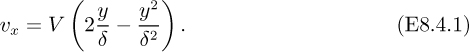
This particular choice has the further advantage that it exactly reproduces the well-known parabola when point C is reached.
On the basis of this velocity profile, the following useful quantities can be determined, in which it is convenient to define a fraction α:
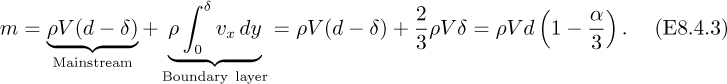
Momentum flux
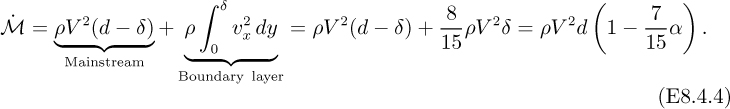
Wall shear stress

Mean/mainstream velocity relation
Bernoulli’s equation in the mainstream

Now perform a momentum balance in the x direction on the rectangular element shown in Fig. E8.4.2, situated between the wall and centerline, noting that at the centerline there is zero velocity gradient and hence zero shear stress:

Differentiation of Eqn. (E8.4.4) with respect to x gives:

After making the appropriate substitutions, Eqn. (E8.4.9) yields an ordinary differential equation for α as a function of x:

Separation of variables and integration between the channel inlet and the location at which the boundary layer reaches out to the centerline gives:

That is, the dimensionless entrance length is directly proportional to the Reynolds number (based in this case on half the separation between the plates):
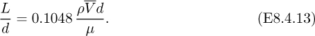
For flow in a pipe of diameter D, the corresponding result is L/D ![]() 0.061 Re, in which Re = ρ
0.061 Re, in which Re = ρ![]() D/μ.
D/μ.
8.8. The Lubrication Approximation
This chapter continues with situations not unlike those encountered in the earlier boundary-layer analysis—namely, in which there is a dominant velocity component in one direction.
Consider the simplified cross-sectional view of a journal bearing, shown in Fig. 8.8(a). The heavy shaft of weight W per unit length rotates counterclockwise inside the housing, the two being separated by a thin lubricant film of viscous oil. Although the pressure at the two extremities of the oil film is atmospheric (p = 0, say), the following analysis will show that the rotation of the shaft induces a significant pressure increase between these two points—enough to support the weight of the shaft. Observe that when equilibrium is reached, the shaft and housing are not concentric, so that the oil film, whose thickness is greatly exaggerated in Fig. 8.8(a), becomes thinner in the direction of rotation. The shaft becomes off-center automatically and to a very small degree.

Fig. 8.8 (a) Journal bearing, with exaggerated thickness of the oil film, and (b) magnified view of film.
Because the oil film is very thin, the analysis can justifiably be expedited by “unwinding” the film and considering it to be wedge-shaped, contained between an upper surface (the shaft) moving with velocity V and a lower stationary surface (the housing), an enlarged portion of which is shown in Fig. 8.8(b). Observe that the oil tends to be squeezed into an ever-narrowing space, and that this is the basic cause of the increased pressure.
A similar situation—that of a thrust bearing—is shown in Fig. 8.9. In this case, the horizontal thrust W of an axle is resisted by a series of wedge-shaped segments, arranged in a circle on a fixed end plate, adjacent to which is a disk attached to the rotating axle. The fluid between the disk and segments does not have to be oil—it will probably be air in the majority of cases.
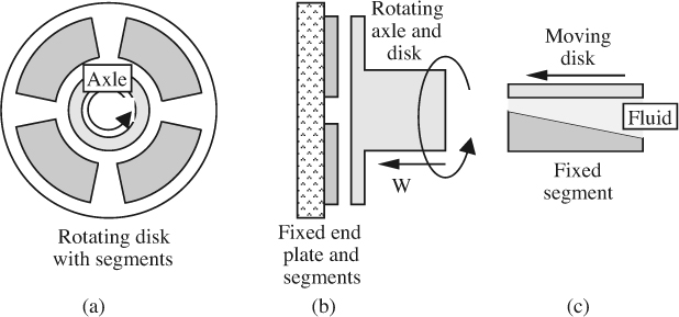
Fig. 8.9 Details of thrust bearing: (a) head-on view of end plate with segments; (b) side view of axial section; (c) the motion of the disk relative to one of the fixed segments on the end plate.
To proceed with the analysis of the journal bearing, make the following simplifying assumptions, all of which can be justified by arguments similar to those made when analyzing the formation of a boundary layer on a flat plate:
1. There is a dominant velocity component in one direction—x for example.
2. Pressure is only a function of the x coordinate—that in the primary flow direction, and not of the transverse coordinate y. That is, p = p(x) and ∂p/∂y = 0.
3. Inertial and gravitational terms are negligible in comparison with the two dominant effects of pressure and viscous forces.
4. There is no flow in the z direction, normal to the plane of the diagram. This is a poor assumption in some cases, not considered here, in which there is a continuous leakage of makeup lubricant along the direction of the shaft (with a corresponding injection of lubricant in the vicinity of the bearing surface).
Basic equations for flow in a bearing. Item 1 above indicates that only the x momentum balance is needed from the full Navier-Stokes equations:

With the simplifications just listed—known as the lubrication approximation—the momentum balance reduces to:

At the boundaries, the fluid has zero velocity at the fixed lower surface, and moves with velocity V cos θ ![]() V (θ is quite small) at the moving upper surface:
V (θ is quite small) at the moving upper surface:
Double integration of Eqn. (8.86), incorporating these two boundary conditions, leads to the following expression for the velocity profile at any section in the x direction:
Observe the interpretations of the two terms appearing on the right-hand side of Eqn. (8.88):
1. The first term represents Couette flow, in which there is a linear increase in υx, from zero at the stationary lower surface to V at the moving upper surface.
2. The second term corresponds to pressure-driven Poiseuille flow, in which the velocity is zero at the two surfaces, varying parabolically between them.
The problem is not yet solved, because dp/dx is unknown. Therefore, now focus attention on determining how the pressure—and hence its gradient—varies over the length of the bearing. To start, the volumetric flow rate of lubricant along the bearing is obtained by integrating the velocity across the film:

Observe again the Couette and pressure-induced contributions to the flow rate. Unless there is leakage of lubricant normal to the plane of Fig. 8.8 (as could occur in a truly two-dimensional bearing), Q must remain constant. Thus, setting dQ/dx = 0 immediately leads to the differential equation that governs the variation of pressure along the bearing:
which is an example of Poisson’s equation, and in which the expression on the right-hand side is effectively a “generation” term, which serves to boost the pressure. Note that the relative velocity of the two surfaces (V) and the steepness of their inclination (dh/dx) are important factors in causing the pressure increase.
Pressure variation in the bearing. In a bearing, viscous friction causes temperature variations, so the viscosity depends on position. In such cases, Eqn. (8.90) can always be solved numerically for the pressure. However, to proceed further analytically at an introductory level it is necessary to make the following simplifying assumptions:
1. The fluid viscosity μ is constant.
2. The inclination dh/dx is also constant.
3. Eventually, a mean film thickness, hm, may be introduced for further simplification.
After defining a positive quantity:
(note that dh/dx is negative), the pressure equation becomes:
which, when integrated once, gives:
in which c1 is an integration constant.
A precise integration of Eqn. (8.93)—see Problem 8.10—demands that the exact expression for the film thickness, h = h(x), be used. An approximate answer may be obtained by assuming that h maintains its mean value, hm, in which case we obtain:

The boundary conditions on the pressure are that it is zero at the beginning (x = 0) and end (x = L) of the film, giving:
From Eqns. (8.94) and (8.95), the pressure obeys a parabolic distribution between the two end points:
which is also sketched in Fig. 8.10 as curve A, with a maximum p at the center.

Fig. 8.10 Pressure variation along the lubricant film. Curves A and B are for the simplified (Eqn. (8.96)) and exact (Problem 8.10) methods, respectively.
The mean pressure in the lubricant film is readily obtained by integration as:

in which pmax is the maximum pressure, which occurs (in our simplified treatment) at x = L/2. In reality, if the assumption of h ![]() hm is not made, the point of maximum pressure will be shifted somewhat to the right of the midpoint.
hm is not made, the point of maximum pressure will be shifted somewhat to the right of the midpoint.
Recalling the original curved nature of the surfaces, the total weight per unit length of the shaft that can be supported by the pressure generated in the lubricant film is:

in which φ is the angle between the vertical and the line drawn from the center of the bearing to the point distant by x from the thicker end of the film. Insertion of representative values (including a thin film thickness) will show that W can become quite appreciable.
Since the distribution of pressure is now known approximately, its gradient is:
which can be substituted into the original expression, Eqn. (8.88), for the velocity profile, giving:

Eqn. (8.100) is plotted in Fig. 8.11 at three representative locations along the bearing.

Along the moving surface the velocity is, of course, V. Observe that at the midpoint the velocity profile is purely Couette in nature, since the pressure gradient dp/dx is zero at this location. However, Fig. 8.10 shows that there are significant pressure gradients at x = 0 and x = L, and these create additional Poiseuille-type components at these locations. At the “exit” (x = L), the velocity profile is enhanced beyond its Couette value, whereas at the “inlet” (x = 0) it is reduced, and there is indeed some backflow occurring. In practice, there will be lubricant injected into the film in order to make up for the amounts leaking out at the end locations. The modification of the velocity profile by the pressure gradient is similar to that shown in Fig. 8.6 for the separation of a boundary layer.
Example 8.5—Flow in a Lubricated Bearing (COMSOL)
Consider the situation in Fig. E8.5.1, in which one inclined plate (surface 3) moves at a velocity V relative to a stationary plate at y = 0, the intervening space being occupied by a Newtonian fluid of density 1,000 and viscosity 1.0. The velocity components of the moving plate are u0 = 0.05 in the x direction and υ0 = –0.01 in the y direction. The other three boundary conditions (on surfaces 1, 2, and 4) are shown in Fig. E8.5.1. The two “ends,” at x = –1.4 and x = 1.4, are exposed to a pressure of p = 0. All units are mutually consistent. In reality, a bearing would have a much smaller mean thickness/length ratio, but the present choice allows the main features to be displayed without “stretching” the y coordinate.
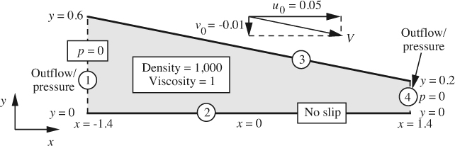
Solve for the streamlines, the pressure distribution, and the variation of pressure along the straight line between midpoints of the opposite “ends”—between points (–1.4, 0.3) and (1.4, 0.1).
Solution
1. In COMSOL, choose the sequence New, Chemical Engineering Module, Momentum Balance, and Incompressible Navier-Stokes.
2. Use the line tool to draw the trapezoid outlining the shaded region in Fig. E8.5.1, noting that the coordinates of the vertices are (–1.4, 0), (1.4, 0), (1.4, 0.2), and (–1.4, 0.6). Remember to terminate at the last point either by right-button click anywhere (PC) or by Control-click (Macintosh).
3. Under Physics/Boundary Settings, set the indicated boundary conditions on boundaries 1, 2, 3, and 4.
4. Under Physics/Subdomain Settings, indicate that ρ = 1,000 and η = 1.
5. Initialize and refine the mesh, and solve the problem.
6. Under Postprocessing, make appropriate choices in the Plot Parameters pulldown menu to generate the following:
(a) A picture that shows 20 streamlines.
(b) A surface plot of the pressure distribution.
(c) A cross-section plot of the pressure between the points (–1.4, 0.3) and (1.4, 0.1). Here, you will need to choose the Line/Extrusion option in the Cross-Section Plot Parameters window.
Discussion of Results
The COMSOL results are shown in Figs. E8.5.2–E8.5.4. The first of these displays the streamlines. In the upper part of the left-hand side, and for almost all of the right-hand side the motion is from left to right, driven by the moving upper plate. But much of the left-hand region is occupied by a clockwise-rotating vortex-type flow; in the bottom half of this vortex, the reason for the flow in the negative x direction is readily seen by examining Fig. E8.5.3, which shows the following important features:
(a) A pressure that essentially depends only on x and not on y—a fact that is at the heart of simplified treatments of boundary-layer and lubrication-type flows.
(b) A high-pressure zone centered at about x = 0.75. The maximum pressure is approximately p = 2.2.
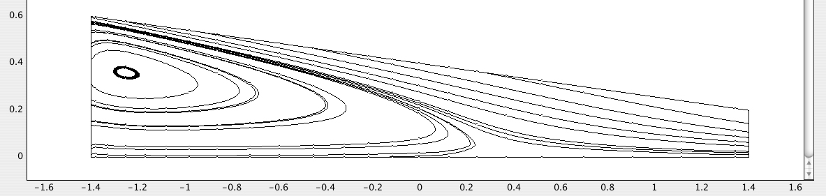
Fig. E8.5.2 Streamlines: in the left-hand half the flow is clockwise, and in the right-hand half it is from left to right. The thin straight line joining points (–1.4, 0.3) and (1.4, 0.1) was added automatically when the pressure cross-plot requested in Item 6(c) above (see Fig. E8.5.4) was made.
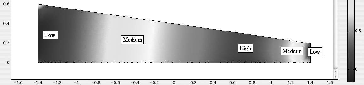
Fig. E8.5.3 A two-dimensional representation (the original being in color) showing the pressure distribution, the approximate magnitudes of which have been added.
Fig. E8.5.4 clearly shows the pressure variation between the midpoints of the two ends—between points (–1.4, 0.3) and (1.4, 0.1). The variation is broadly parabolic but with a peak that is noticeably skewed towards the right of the center.
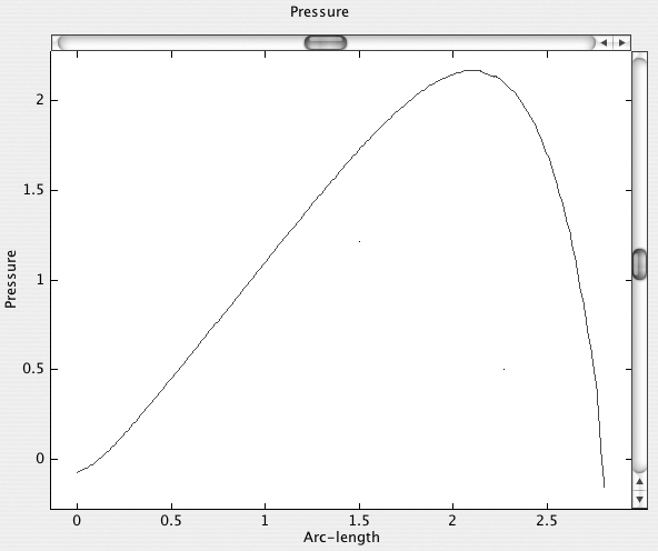
Fig. E8.5.4 Cross-plot of the pressure between midpoints of the two ends, (–1.4, 0.3) and (1.4, 0.1).
8.9. Polymer Processing by Calendering
Calendering is the process of forming a continuous sheet by forcing a semi-molten material through one or more pairs of closely spaced counterrotating rolls. Calendering was first used—and is still used extensively—in the rubber industry. In the plastics industry, the most commonly used plastic that is calendered (about 80–85% of the total) is PVC, both soft (flexible PVC) and hard (rigid PVC). Other plastics that are calendered are mainly LDPE, HDPE, and PP.
Two main benefits can accrue to the calendered material:
1. It is formed to an accurate final thickness.
2. Depending on the nature of the surface of the rolls, a smooth, rough, or patterned surface is imparted to the finished sheet.
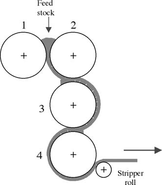
Referring to Fig. 8.12, heat-softened, but not fully molten, material is constantly fed into the nip of rolls 1 and 2. Complete melting and some mixing of additives (such as plasticizers, stabilizers, fillers, lubricants, and colorants) occurs in the first nip, where the stock also warms up. Shear effects also occur because roll 2 normally runs somewhat faster than roll 1—to encourage the band (the film produced) to stick to roll 2 so that it progresses down the rolls. The roll temperatures increase slightly from 1 to 3, but roll 4 is slightly cooler than roll 3 to encourage the film to strip easily off roll 4. The nip gaps get progressively smaller and that between rolls 3 and 4 should be almost the same as the final film thickness.
6 Mr. Ellis is a polymer testing and processing specialist at The Petroleum and Petrochemical College, Chulalongkorn University, Bangkok. We thank him for supplying all of the practical information on calendering in this section.
The functions of the three nips are:
1. First nip (between rolls 1 and 2). The feed rate through the calender is determined here. This is also related to the material residence time, which is relatively short (good for PVC, which is easily degraded). Roll speeds obviously influence these factors.
2. The second nip (between rolls 2 and 3) functions as a kind of metering device. The melt gets spread along the rolls axially to its final width here, although most axial spreading should occur in the first nip.
3. The third nip (between rolls 3 and 4) is the final shaping step, analogous to a sheet extrusion die.
With its highly polished precision rolls and ancillary equipment, calendering is a very capital-intensive operation. Typical operating conditions are:
1. Roll diameters are generally in the range of 40–90 cm. Roll lengths are typically from 1–2.5 m, corresponding to a length-to-diameter ratio between 2 and 3.
2. Roll separation (“nip gap size”) varies from one pair of rolls to the next but is adjustable up to about 5 mm. Production calenders turn out sheet with a thickness tolerance of ±0.005 mm over the width of the final sheet, whose thickness is usually 1 mm at most.
3. Roll speeds. Linear line speeds are generally in the range 30–120 m/min (100– 400 ft/min) for production machines. The actual roll speeds are fairly low (e.g., 20 rpm). If, for example, the roll diameter is 70 cm and the rotational speed is 20 rpm, this works out to be 44 m/min linear line speed. Calendering typically involves shear rates from 1–100 s–1.
During calendering, the melt needs to be fairly viscous, otherwise it can run all over the calender bowls. But conversely, too high a viscosity will create excessive roll bending due to the high pressure created between the rolls (up to 800 bar)! Typical viscosities would correspond to a MFI of 1 or 2, equivalent to a melt viscosity of between 103 and 104 N s/m2 (104 to 105 poise).
An idealized representation of calendering is shown in Fig. 8.13, in which two counterrotating rollers with angular velocities ω, radii R, and closest separation 2H are employed for reducing the thickness of a sheet of material, ideally assumed to have a Newtonian viscosity μ, from an initial value of 2H1 to a final value 2H2.
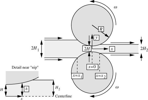
![]() key quantity in the analysis is the distance h = h(x) of either roller from the centerline y = 0. To make reasonable headway without resorting entirely to numerical methods, it is necessary to assume that x/R is small, which is approximately true in the location of greatest interest (the “nip” region), where the separation of the rollers is small and the pressure gradients are the highest. Application of Pythagoras’s theorem leads to:
key quantity in the analysis is the distance h = h(x) of either roller from the centerline y = 0. To make reasonable headway without resorting entirely to numerical methods, it is necessary to assume that x/R is small, which is approximately true in the location of greatest interest (the “nip” region), where the separation of the rollers is small and the pressure gradients are the highest. Application of Pythagoras’s theorem leads to:
in which the approximation ![]() has been made for small values of ε = x/R.
has been made for small values of ε = x/R.
The situation and assumptions are very similar to those studied in the previous section, and the lubrication approximation again leads to pressure only being a function of x, together with the governing equation:

The boundary conditions on the velocity υx are that at the extremities of the gap it is approximately the same as the peripheral velocity of the rollers (at y = h), and that there is symmetry about the centerline of the sheet (y = 0):

It is then easy to show that:

in which the pressure gradient is, for the present, unknown, and that the flow rate per unit depth, normal to the plane of Fig. 8.13, is:

which can be rearranged to give the pressure gradient as:
Now focus on the point, x = x2, where the calendered sheet leaves the rollers with a half thickness of y = H2. From then on, the pressure is everywhere constant, since the sheet is exposed to the atmosphere. Thus, it is reasonable to suppose a flat velocity profile at the point of departure, the same as in the sheet after it has left the rollers. Thus, the flow rate is the peripheral velocity times the thickness:
which amounts to saying that the pressure gradient dp/dx is zero at this stage. Eqn. (8.106) then becomes, after invoking Eqn. (8.101):

In order to proceed further, the following integrals will be needed, which in this case have conveniently been obtained from the computer program “Maple”:


Noting that the pressure has fallen to zero at the point of departure from the rolls, Eqn. (8.108) integrates to:
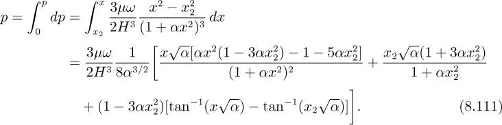
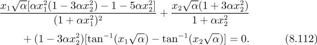
For a specified inlet sheet thickness 2H1, the corresponding value of x1 will be known from Eqn. (8.101). The value of x2 (the point at which the sheet leaves the rolls) can then be determined by using Eqn. (8.111) in conjunction with the upstream boundary condition, p(x1) = 0 (atmospheric pressure), by solving the following equation for x2:
Example 8.6—Pressure Distribution in a Calendered Sheet
To illustrate the preceding analysis, evaluate the point of departure, and the pressure distribution, for a calendering operation in which R = 0.35 m, H = 0.00025 m, and x1 = –0.01 m. The rolls rotate at 20 rpm, and the viscosity of the melt is 0.5 × 10⁴ P.
Solution
First, note that α = 1/2HR = 1/(2 × 0.00025 × 0.35) = 5,714 m–2. The solution of Eqn. (8.112) can then be effected by any standard numerical rootfinding technique. The “Goal-Seek” feature of the Excel spreadsheeting application gives the downstream distance before separation as x2 = 0.00403 m.
When x2 has thus been found, Eqn. (8.111) then gives the complete pressure distribution, which can again be evaluated with the aid of a spreadsheet. The results are shown in Fig. E8.6, which actually shows a closely related value as the ordinate (namely, the expression in the large brackets in Eqn. (8.111)):
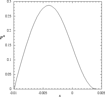
Observe that the pressure rises from zero at the inlet, to a maximum upstream of the “nip,” and then declines to zero as the sheet leaves the calender. In accordance with an earlier observation, note that the pressure gradient is zero at the exit.
The angular velocity of the rolls is ω = 2π × 20/60 = 2.09 rad/s. Since the maximum value of p* is about 0.288, the maximum pressure between the rolls is:

As mentioned previously, the maximum pressure can be simply enormous.
8.10. Thin Films and Surface Tension
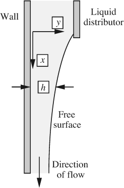
This chapter continues with situations not unlike those encountered in the earlier boundary-layer analysis—namely, in which there is a dominant velocity component in one direction, and also in which surface tension may be important. Fig. 8.14 shows a thin liquid film, of density ρ and viscosity μ, after it leaves the distributor at the top of a wetted-wall column, which can be used for gas-absorption and reaction studies in relatively simple geometries. Of interest here is the shape of the free surface once the liquid is free of the influence of the distributor, a situation that has been investigated both theoretically and experimentally by Nedderman and Wilkes.7
7 R.M. Nedderman and J.O. Wilkes, “The measurement of velocities in thin films of liquid,” Chemical Engineering Science, Vol. 17, pp. 177–187 (1962). This investigation was started by Prof. Terence Fox, to whom this book is dedicated, and represents the only case known to the author in which the legendary Prof. Fox initiated any doctoral research (see the Preface).
Since the film is thin, curvature effects of the cylindrical tube wall can be neglected, and the problem can be solved in x/y coordinates, leading to the following parabolic velocity profile:
Here, Q is the total volumetric flow rate (per unit depth, normal to the plane of the figure), h is the local film thickness, and y is the coordinate measured from the wall into the film.
Now perform a momentum balance on an element of the film, shown in Fig. 8.15, analogous to a similar treatment in Section 8.2 for the analysis of boundary-layer flow. The surface BC is taken to be just on the liquid side of the liquid/air interface, and will have a pressure acting normally on it, whose mean value is p + (dp/dx)(dx/2).
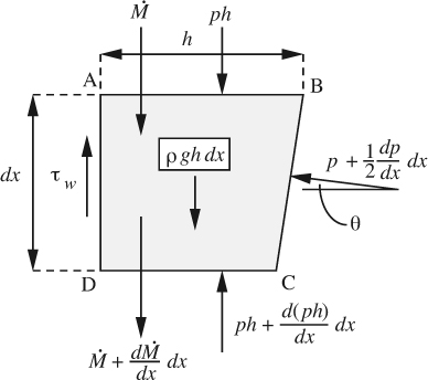
If ![]() is the x convected momentum flux in the film, a downward steady-state momentum balance gives:
is the x convected momentum flux in the film, a downward steady-state momentum balance gives:
Here, the sin θ term recognizes that the normal force on the surface BC must be resolved in the vertical direction. After substituting for the wall shear stress, noting that sin θ ![]() –dh/dx, and neglecting a second-order differential quantity (dx)2, Eqn. (8.114) simplifies to:
–dh/dx, and neglecting a second-order differential quantity (dx)2, Eqn. (8.114) simplifies to:
Now observe that the momentum flux per unit depth in the film is:
Also note that the pressure p in the film will in general differ from the pressure p0 = 0 in the gas outside the liquid film because of surface tension σ. The pressure decreases as we proceed across the free surface into the film, by an amount that equals the product of the surface tension and the curvature of the film. Provided that |dh/dx| ≪ 1, and observing the expression for curvature in Appendix A, the result may be simplified:

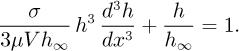
That is, Eqns. (8.115)–(8.117) lead to a third-order nonlinear ordinary differential equation that governs variations in the film thickness, in which ν = μ/ρ is the kinematic viscosity:
In general, Eqn. (8.118) cannot be solved analytically. However, Nedderman and Wilkes (loc. cit.) do give solutions for the following limiting cases:
1. For negligible surface tension, the analytical solution shows that the film thickness steadily approaches its final steady asymptotic value, h∞ =(3Qμ/ρg)1/3.
2. For finite surface tension, and with the film thickness near h∞, an approximate solution for the film thickness shows that the expression for h consists of two parts:
(a) A disturbance that decays downstream.
(b) A series of standing waves that become amplified downstream. That is, the film tends to become unstable. If the wave amplitude is significant, however, the assumption of a parabolic velocity profile becomes questionable—in other words, the above simplified theory cannot be “pushed” too far.
Surface-tension forces can play vital roles in stabilizing or destabilizing coating operations and paint leveling, as suggested by Problems 8.6 and 8.13.

Problems for Chapter 8
Unless otherwise stated, all flows are steady state, with constant density and viscosity.
1. Boundary layer with linear velocity profile—E. Review the simplified treatment of Section 8.2 for the boundary layer on a flat plate. Repeat the development with the following expression for the velocity profile in the boundary layer, instead of Eqn. (8.9):
You should obtain expressions for both δ/x and cf, similar to Eqns. (8.16) and (8.17). Also see Table 8.1. What are the merits and disadvantages of this linear velocity profile?
2. Boundary layer with suction—M. Fig. P8.2 shows the development of a boundary layer on a porous plate, in which fluid is sucked from the boundary layer with a superficial velocity υs normal to the plate. (This arrangement has been proposed for airplane wings, in order to reduce the drag by preventing the boundary layer from becoming turbulent at high Reynolds numbers.)
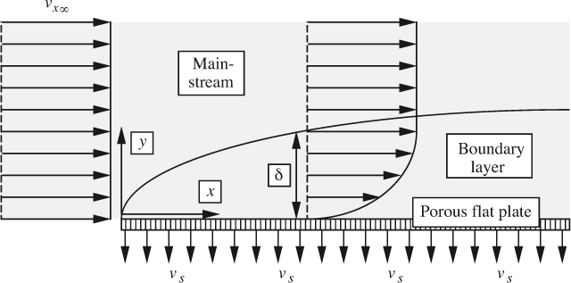
Use the simplified treatment to prove that the momentum balance of Eqn. (8.4) becomes:
Assuming a velocity profile of the form υx/υx∞ = 2ζ – ζ2, where ζ = y/δ, derive an expression for δ as a function of x. Hence, show that the boundary layer will eventually reach a constant thickness—which no longer changes with distance x—and derive an expression for this limiting thickness.
3. Tank draining with boundary layer—M. For a laminar boundary layer on a flat plate, the solution in Section 8.2 gave the following expression for the wall shear stress at a point distant x from the leading edge:
Derive an expression for the total drag force F exerted by a plate of length L on the fluid, per unit distance normal to the plane of Fig. 8.3. Your answer should give F in terms of υx∞, L, ρ, and μ or ν.
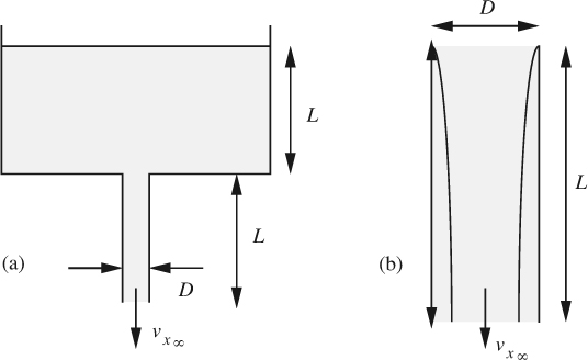
As shown in Fig. P8.3(a), a viscous liquid is draining steadily from a largediameter tank. As it enters the pipe of diameter D and length L, it has a flat velocity profile, and a thin laminar boundary layer subsequently forms, as in Fig. P8.3(b). Derive an expression for the velocity of the liquid υx∞ in the mainstream, in terms of any or all of D, L, g, ρ, and μ. Assume that the boundary layer is sufficiently thin so that υx∞ is essentially constant; also, since the velocities are small, neglect any inertial terms in a momentum balance. Evaluate υx∞ if L = 1m, D = 0.1 m, ρ = 1,000 kg/m3, g = 9.81 m/s2, and μ = 1 kg/m s.
4. Power for the “Queen Mary”—M. The RMS Queen Mary embarked on her maiden transatlantic voyage from Southampton, England, on May 27, 1936. On the crossing to New York, she achieved an average speed of 29.13 knots (1 knot = 1.15 miles/hour). Her length at the waterline was 1,004 ft, with a draft of 38.75 ft and a beam (width) of 118 ft. Anybody who has been underneath the Queen Mary, when in dry dock, can attest that the bottom of the ship is almost completely flat.
Estimate the horsepower needed to overcome skin friction on the Queen Mary’s maiden voyage, and compare with the total of 160,000 HP that was nominally delivered to the quadruple screws of the ship. Assume a density of 64.0 lbm/ft3 and a viscosity of 3.45 lbm/ft hr for seawater. Clearly state any reasonable simplifying assumptions.
5. Pressure in a bearing—E. The shaft in a journal bearing has a diameter of 2 ft and rotates at 60 rpm. The lubricant film extends all the way around the lower half of the shaft, with maximum and minimum thicknesses of 0.003 and 0.001 ft, respectively. If the viscosity of the lubricant is μ = 1, 000 cP, estimate the mean pressure (psi) in the film.
6. Coating a moving substrate—M. A continuous strip of a flexible metal substrate is being pulled to the right with a steady velocity V as it leaves a reservoir of a protective liquid polymer coating of viscosity μ and surface tension σ, as shown in Fig. P8.6.
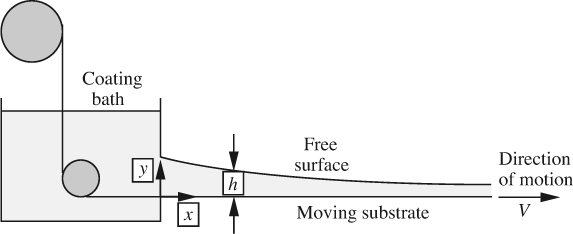
Assuming that pressure and viscous forces dominate, what is the simplified x momentum balance? If the pressure in the liquid film only depends on x, show that the velocity profile is given by:
where h = h(x) is the local film thickness. If surface tension is important, why is dp/dx in the film positive for the free-surface shape as drawn in Fig. P8.6? Sketch the resulting velocity profile.
If the final thickness of the coating is h∞, prove that the intermediate film thicknesses obey:
7. Wetted-wall column without surface tension—M. For the film on the wetted-wall column discussed in Section 8.10, variations of film thickness are governed by the differential equation:
Consider the situation in which surface tension is negligible.
The analytical solution of Eqn. (P8.7.1) is somewhat complicated. However, show that if the film thickness is not too far from its asymptotic value (h/h∞ ![]() 1), the solution may be approximated by:
1), the solution may be approximated by:
in which h∞ = (3Qμ/ρg)1/3 and c is a constant of integration. Give a physical interpretation of Eqn. (P8.7.2).
8. Wetted-wall column with surface tension—D. Consider the film on the wetted-wall column discussed in Section 8.10, in which the variations of film thickness were governed by the differential equation:
Supposing that the film thickness is close to its steady value (that is, h = h∞ + ε, where ε ≪ h∞, and h∞ = (3Qμ/ρg)1/3), prove that the governing equation becomes:
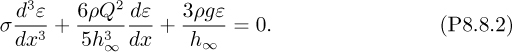
Now attempt a solution of the form:
for which a representative term is:
and derive the corresponding cubic equation in δ. Now form (δ – α)(δ – β)(δ – γ) = 0, in which:
and compare it with the cubic equation. Hence, verify that the three roots for δ are those given in Eqn. (P8.8.5), where i = ![]() , both η and ζ are real, and η is positive. Hence, show, by noting that b and c must be complex if the final solution is to be real, that:
, both η and ζ are real, and η is positive. Hence, show, by noting that b and c must be complex if the final solution is to be real, that:
in which a, κ, and λ are unknown real constants. Give a physical interpretation of each of the terms in Eqn. (P8.8.6).
9. Alternative thin-film momentum balance—E. Perform a careful momentum balance on an element of a thin liquid film, as in Fig. 8.14. However, now take the surface BC to be just on the air side of the liquid/air interface, so the pressure acting on it is p0 = 0. Make sure that you obtain the same final result, namely, Eqn. (8.115). There will now be surface tension forces σ (per unit depth normal to the plane of Fig. 8.14) acting tangentially along the interface, and these will have to be resolved in the vertical direction—through angles that are marginally different at B and C.
10. Exact pressure distribution in a lubricant film—D. In Section 8.8, the final expression for the pressure distribution in the lubricant film, Eqn. (8.96), assumed that the film thickness h maintained its mean value hm. Refine the solution by conducting an exact integration of Eqn. (8.93), now with the film thickness h(x) varying linearly between h0 (at x = 0) and hL (at x = L) according to:
Prove that the pressure distribution is given by:
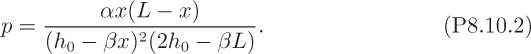
Use a standard computer application such as Excel to plot ph3m/αL2 against x/L, for βL/hm = 0, 0.1, and 0.5. Explain your observations qualitatively.
11. Trying to keep warm—M. You are walking along the street in Chicago when the 0 °F air is moving down the street with a “mainstream” velocity of υx∞ = 30 mph. At each block, as the air impacts the corner of a building, a boundary layer builds up along the side of the building, just as it does on a flat plate.
To avoid getting too cold, you walk very close to the building, hoping to stay inside the boundary layer. At what minimum distance from the corner can you be guaranteed that the boundary layer will be at least 2 ft wide? For air, ρ = 0.086 lbm/ft3, μ = 0.0393 lbm/ft hr.
12. Velocity profiles in calendering—M. For the calendering problem for which the pressure distribution is shown in Fig. E8.6, use a spreadsheet application to plot the velocity profiles at x = –0.05, –0.025, 0, and 0.0225. A plot of υx/ω versus y/h is recommended. Comment briefly on your results.
13. Leveling of a paint film—M. The problem of the leveling of paint films after they have been sprayed on automobile body panels is becoming quite important as increased-solids paints of lower polymeric molecular weight are being mandated by the government.8 An idealized situation is shown in Fig. P8.13, in which a paint film, of density ρ and Newtonian viscosity μ, has at an initial time t = 0 a nonuniform thickness h = h0(x). You are called in as a consultant to help derive a differential equation, whose solution would then indicate how h subsequently varies with time t and position x.
8 This problem follows part of the doctoral research of Richard Blunk of the General Motors Corporation; his help and insight are gratefully acknowledged.

You may make the following assumptions:
(a) Because the paint film is baked in an oven, there will be known temperature variations and hence known changes in the surface tension σ along the surface of the film; these give rise to a known shear stress (τyx)y=h = μ(∂υx/∂y)y=h = ∂σ/∂x at every point on the surface.
(b) Surface tension causes the pressure to change from atmospheric pressure (zero) just outside the film to a different value just inside the film, in exactly the same manner as in Eqn. (8.117). In addition, gravity is now important, and the pressure increases hydrostatically from just inside the free surface to the body panel.
(c) The usual lubrication approximation/boundary layer theory still holds; that is, inertial effects can be neglected, and the flow in the film is mainly in one direction, so that you need only be concerned with the velocity component υx.
Now answer the following:
(a) Derive an expression for the pressure p at any point in the film, as a function of ρ, σ, g, h, x, and y. Then form ∂p/∂x, and show that this is not a function of y.
(b) To what two terms does the x momentum balance simplify? Integrate it twice with respect to y, apply the boundary conditions, and show that the velocity profile is given by:
(c) Integrate the velocity to obtain an expression for the flow rate Q in the paint film.
(d) By means of a mass balance on an element of height h and width dx, prove that variations of the film thickness h with time are related to variations of the flow rate Q with distance by:
(e) Indicate briefly what you would next do in order to obtain a differential equation governing variations of h with x and t. (However, do not perform these steps.)
14. A check on the Blasius problem—M. Concerning the mathematics leading up to the solution of the Blasius problem, first check Eqn. (8.48). Then verify that substitution of υx and υy and the derivatives of υx from Eqns. (8.47) and (8.48) into Eqn. (8.38) leads to the following ordinary differential equation:
subject to the boundary conditions:
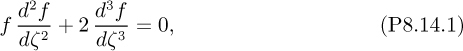
15. Numerical solution of the Blasius problem—D. This problem concerns the numerical solution of the third-order ordinary differential equation and accompanying boundary conditions of Eqns. (8.49)–(8.51), also restated in Problem P8.14 above.
(a) Verify that by defining new variables z = ζ, f0 = f, f1 = df/dz, and f2 = d2f/dz2, Eqn. (8.49) can be expressed as three first-order ordinary differential equations:
subject to the boundary conditions:
(b) As discussed in Appendix A, use a spreadsheet to implement Euler’s method to solve Eqns. (P8.15.1) subject to boundary conditions (P8.15.2), from z = 0 to z = 10 (which latter value is effectively infinity). (Any other standard software for solving differential equations may be used instead.) A step-size of Δz = 0.1 or even smaller is recommended, otherwise Euler’s method is not very accurate. Try different values for Δz in order to get a feel for what is happening.
(c) You will need to supply the “missing” boundary condition for f2 at z = 0, so that f1 is very close to the actual boundary condition f1 = 1 at z = 10. If you are using Excel, you will find the “Goal-Seek” feature under the “Formula” pull-down menu to be very helpful.
(d) When all is working satisfactorily, add another column for the dimensionless y velocity, and then plot the two dimensionless velocities against the dimensionless distance from the wall. Clearly label everything, and check your results against those given in Fig. 8.5.
16. Developing boundary layer—M. Consider a cylinder of radius a that starts to rotate at t = 0 with an angular velocity of ω in an otherwise stagnant liquid of kinematic viscosity ν. We wish to calculate the thickness δ = δ(t) of the boundary layer that starts to build up around the cylinder and grows with time. Since δ a, we may approximate the situation in x/y coordinates, as shown in Fig. P8.16, in which U = aω is the velocity of the surface of the cylinder, and y is the radially outward direction.
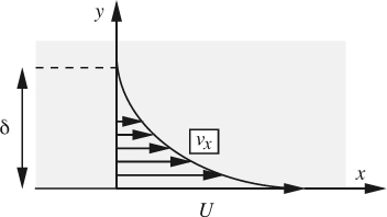
If the pressure is uniform everywhere, what justification is there for assuming that υx obeys the equation:
To solve Eqn. (P8.16.1) approximately, use the similarity approach, in which the velocity profile is assumed to be of the following form for all values of δ:

(a) Explain why the form of υx given by Eqn. (P8.16.2) is reasonable.
(b) By substituting for υx from Eqn. (P8.16.2) into Eqn. (P8.16.1) and integrating both sides from y = 0 to y = δ, and then integrating the resulting differential equation in δ and t, prove that the boundary-layer thickness varies with time according to:
and determine the value of the constant c.
17. Boundary layer on a wire—M (C). As shown in Fig. P8.17, a stream of fluid flows with mainstream velocity υz∞ parallel to the axis of a thin cylindrical wire of radius a. Within the laminar boundary layer, which builds up near the surface of the wire, the velocity profile in the fluid is given by υz = υz∞ sin(πr/2 δ), where δ is the boundary-layer thickness, r is the radial distance from the surface of the wire, and z is the axial coordinate. Perform a simplified momentum balance on an element of the boundary layer of axial extent dz.
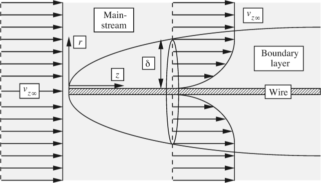
Assume that the wire is very thin, so that in any integrals for mass and momentum fluxes, you may take the lower limit as r = 0. The only time you will require the wire radius a is when you need an area on which the wall shear stress acts.
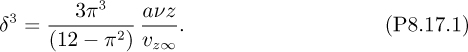
Hence, prove that the thickness of the boundary layer varies with axial distance as:
Rearrange this result in terms of three dimensionless groups, δ/z, a/z, and υz∞z/ν.
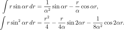
The following integrals may be quoted without proof:
18. Wetted-wall column with boundary layer—D (C). Fig. P8.18 shows idealized flow conditions in a wetted-wall column, which consists of two wide parallel plates of length L separated by a distance h. The insides of the plates are covered by uniform thin films of liquid, whose surfaces move down with velocity W. Air of density ρ and viscosity μ enters the bottom of the column from a large reservoir at a small pressure P above that at the top of the column.
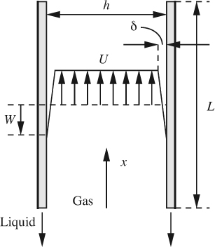
The value of W is unaffected by the airflow, whose pattern at any section consists of a central core of uniform upward velocity U, and a boundary layer of thickness δ = δ(x), across which the velocity varies linearly between the central core and the liquid film.
Show that δ = h(U – U0)/(U + W), where U0 is the value of U at the bottom of the column. Also prove that the momentum passing across any section is, per unit depth, normal to the plane of the diagram:

Outline—but do not attempt to carry to completion—the steps that are needed to determine U0 as a function of L, h, W, ρ, and μ. Hint: Consider the development of Example 8.1. Ignore any gravitational effects.
19. Isokinetic sampling of a dusty gas—D (C). Consider the boundary layer of thickness δ that develops along a flat plate for laminar flow with mainstream velocity υx∞ in a fluid of density ρ and viscosity μ.
(a) If the velocity profile in the boundary layer is of the form:
derive an expression that gives the ratio δ/x as a function of the Reynolds number Rex = ρυx∞x/μ, based on the distance x from the leading edge. If needed, you may quote an integral momentum balance without proof.
(b) Hence, prove that the corresponding expression for the local wall shear stress is given by:
(c) If the mean wall shear stress between x = 0 and x = L is defined by:
derive an expression for ![]() that is very similar to Eqn. (P8.19.2), except that the Reynolds number ReL = ρυx∞L/μ, based on the total length, L, now appears.
that is very similar to Eqn. (P8.19.2), except that the Reynolds number ReL = ρυx∞L/μ, based on the total length, L, now appears.
(d) Fig. P8.19 shows a probe of length L and internal diameter d for sampling a gas of density ρ and kinematic viscosity ν that contains fine dust particles. Upstream of the probe, the mainstream velocity is υx∞, and it is essential that the velocity at the inlet A of the probe must be the same, otherwise a biased sample will occur. (For example, if the velocity at A exceeds υx∞, some dust particles, because of their inertia, will deviate little from their path and will not be drawn into the sampling tube.) To achieve this condition of “isokinetic” sampling, the pressure at B must be reduced below that at A, to compensate for the wall shear stress that builds up in the boundary layer that coats the inside wall of the sample probe. Derive an approximate expression that gives the required pressure difference (pA – pB) for isokinetic sampling.
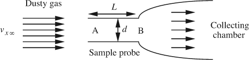
20. Boundary layer in stagnation flow—M. Consider the upper half plane (y ≥ 0) of the potential stagnation flow of Example 7.2, and take the x axis to be the surface of the ground, with a vertically downward wind impinging on it. Since viscosity is now important adjacent to the solid surface at y = 0, there will be a developing boundary layer. Noting from symmetry that only x > 0 needs to be studied, the thickness δ = δ(x) of the boundary layer will be a function of the distance from the origin.
Since for the stagnation flow υx = υx∞ = cx, the mainstream velocity is not constant; thus, the pressure p = p(x) will also be a function of location. The y component of the mainstream velocity can be ignored, since υy = –cy, and y is very small.
If the flow is laminar with υx/υx∞ = sin[πy/(2 δ)], perform a simplified momentum balance on an element of the boundary layer and obtain a differential equation that governs δ as a function of x. If the boundary-layer thickness reaches a steady asymptotic value (in which case assume dδ/dx = 0 without solving the differential equation), prove that this value equals ![]()
21. Film-thickness variations—M. In the coating experiment shown in Fig. P8.21, a flexible paper sheet is being withdrawn vertically upward at a velocity V from a bath containing a Newtonian polymeric liquid of viscosity μ, density ρ, surface tension σ, and local thickness h. Assume that a momentum balance gives the following velocity profile:


If the net upward liquid flow rate Q (per unit depth normal to the plane of Fig. P8.21) is zero (as much is being dragged upwards as falls under gravity), derive a differential equation that governs the variation of film thickness h with distance x. Assume steady flow—that is, there are no time derivatives.
If, for large x, the film were to come to a constant thickness h∞, express h∞ in terms of μ, V, ρ, and g.
Suppose that the film thickness deviates by a small amount ε from h∞, so that h = h∞ +ε. Derive a differential equation for ε as a function of x. Try a solution of the form ε = deδx, and obtain an equation from which δ could be calculated (but do not attempt to obtain these values). If needed, 1/[1+(ε/h∞)] ![]() 1 – (ε/h∞).
1 – (ε/h∞).
22. True/false. Check true or false, as appropriate:
(a) A boundary layer is a region in which neither viscous nor inertial terms can be neglected.
T ![]() F
F ![]()
(b) A drag coefficient is a measure of the ratio of viscous to inertial forces.
T ![]() F
F ![]()
(c) In boundary layers, “similarity of velocity profiles” means that the profiles of υx are “stretched” in both the x and y directions.
T ![]() F
F ![]()
(d) In the simplified analysis of a boundary layer on a flat plate, the assumption that υx = y/δ leads to a drag coefficient that is within 5% of that predicted by the more exact Blasius solution.
T ![]() F
F ![]()
(e) In the analysis of boundary layers, Bernoulli’s equation can be used to predict ∂p/∂x if the mainstream velocity υx∞ is known as a function of the distance x.
T ![]() F
F ![]()
(f) The Blasius analysis of the boundary-layer problem converts the equations of motion, which contain partial derivatives, into a second-order ordinary differential equation.
T ![]() F
F ![]()
(g) At the transition from one to the other, a laminar boundary layer is significantly thinner than a turbulent one.
T ![]() F
F ![]()
(h) The relative motion of two surfaces, slightly inclined to each other, can cause appreciable pressure rises in a fluid that is located in the narrow gap between the two surfaces.
T ![]() F
F ![]()
(i) In lubrication analysis, the Couette flow component indicates a parabolic velocity profile.
T ![]() F
F ![]()
(j) In calendering, a knowledge of the entering sheet thickness, together with the geometry of the rolls and their speed, will enable the exiting sheet thickness to be determined.
T ![]() F
F ![]()
(k) For the Blasius problem, dimensional analysis can lead to the exact form of the relation between the drag coefficient and the Reynolds number, apart from a single unknown constant.
T ![]() F
F ![]()
(l) In a lubricant film, the maximum pressure occurs somewhat closer to the end of the film that has the greater thickness.
T ![]() F
F ![]()
(m) In the boundary layer on a flat plate, the flow is entirely parallel to the plate, with zero velocity in the direction normal to the plate.
T ![]() F
F ![]()
(n) In the drag coefficient plot for flow past a sphere, the sudden “dip” at high Reynolds number is because the boundary layer suddenly becomes turbulent.
T ![]() F
F ![]()
(o) In the simplified analysis of a boundary layer on a flat plate, the value of ∂2υx/∂y2 at the plate is zero when υx∞ is constant.
T ![]() F
F ![]()
(p) Boundary-layer separation is likely to occur in flow in a diverging channel.
T ![]() F
F ![]()
(q) Boundary-layer separation is likely to occur in flow of a circular jet of air normal to a flat plate (“stagnation flow”).
T ![]() F
F ![]()
(r) The total shaft weight that can be supported by a lubricant film in a journal bearing increases with decreasing lubricant viscosity.
T ![]() F
F ![]()
(s) The addition of a surface-active agent to decrease the surface tension of a liquid is likely to increase the instabilities in thin-film flow of the liquid.
T ![]() F
F ![]()