
Chapter 13. An Introduction to Computational Fluid Dynamics and Flowlab
13.1. Introduction and Motivation
THE elegant mathematical formulation of the laws governing fluid dynamics has been complete since the late 19th century. In the ensuing half a century, a tremendous amount of progress has been made by famous scientists and fluid dynamicists to provide insights, clarity, and understanding about the solutions to the core equation system, which consists of the continuity, momentum, and energy equations, together with other supporting equations such as the equation of state for gases and rate equations for chemical reactions, etc. For example, Ludwig Prandtl (1875–1953) developed the boundary-layer theory, which is most crucial to advance the state of the art in modern fluid dynamics; G.I. Taylor (1886–1975) contributed enormously to wide-ranging topics such as hydrodynamic instabilities, statistical theory of turbulence, drops and bubbles, and many other areas; and Theodore von Kármán (1881–1963) laid down the foundations of high-speed aerodynamics and aerothermodynamics, in addition to advancing Prandtl’s boundary-layer theory and making numerous other contributions.
But a ponderous fact about fluid dynamics remains unchanged: we are still not able to solve its core second-order nonlinear partial differential equation system analytically, except for some very special cases such as Couette or Poiseuille flow.1
1 Another major obstacle is that we still have very limited knowledge in turbulent flows. The cost of the state of our ignorance cannot be easily measured, but it is definitely a huge number.
In order to obtain approximate solutions to the Navier-Stokes or Euler equations, fluid dynamicists and applied mathematicians had been earnestly developing new theories and tools in numerical analysis along the way. Yet the need for more detailed solutions to the general fluid dynamics equations far exceeded what could be offered by theoretical and numerical analysis alone. Hence the only way for engineers and scientists to patch things up was to rely heavily on experiments in fluids and thermal design—until the arrival of computational fluid dynamics (CFD) in the second half of the 20th century.
CFD combines the fruits of numerical analysis in partial differential equations (PDEs) and linear algebra with the ever-increasing number-crunching power of modern digital computers to solve the governing PDEs approximately. By itself, CFD is not the answer to all questions regarding complex thermal-fluid phenomena, but it has established firmly as an indispensable tool, together with the traditional theoretical and experimental methods, in the analysis, design, optimization, and trouble-shooting of thermal-fluid systems.2
2 From its brief historical background, it should be clear that CFD is more a branch of numerical analysis applied to fluid dynamics than a computer-aided design tool. Hence, the emphasis for successful CFD practitioners lies primarily on their competence in the knowledge of physics of fluids, heat transfer and other associated phenomena, and numerical methods.
In this chapter we can only scratch the surface of the wide-ranging topics in CFD, but we hope the reader will appreciate the importance of the tool so that a further study in CFD is taken as a high priority in preparing and advancing one’s own professional career. Thus, we wish to promote the use of CFD generally, and not any particular software. Of necessity, however, we have had to choose two examples—FlowLab and COMSOL in this and the next chapter. These are but two of a multitude of CFD “packages,” a fairly complete list of which is available at the website http://www.cfd-online.com/Resources/soft.html
CFD applications in chemical engineering. CFD has been extensively used in the chemical, oil and gas, pharmaceutical, and process industries. In part it is due to advances made in the complex physical models (e.g., multiphase flows, chemically reacting flows, and advanced turbulence models, etc.) that have become available in the general-purpose commercial CFD codes.
In comparison with the “traditional” approach of relying on empiricism and experimental correlations for nonuniform or nonequilibrium conditions in the design, scale-up, and operation of processes and unit operations in the chemical industry, CFD analysis provides a more fundamental view of the picture. The numerical computation contains full-field data of velocity, temperature, and species concentrations, etc., which engineers can use to understand better the pattern and visualize the physics of the flow. Furthermore, many “what-if” studies can be performed by CFD to examine quickly the influences of various parameters (physical or geometrical) on flow patterns and system performance.
Chemical engineers have been successfully utilizing CFD as design tool in a wide range of unit operations. A small sampling is listed below:
1. Chemical reactions: fluidized beds, bubble columns, and packed beds.
2. Heat transfer processes: heat exchangers, boilers, and evaporators.
3. Fluid transport processes: pumps, compressors, manifolds, headers, pipes, and valves.
4. Mixing processes: stirred tank reactors, static mixers, in-line mixers, and jetmixed systems.
5. Separation processes: cyclones, scrubbers, precipitators, and filtration systems.
For each of the diverse group of operations, CFD simulation provides detailed field data (and the derived fluxes, stresses, and forces, etc. of interest) in the solution domain. In many cases this valuable insight enables engineers to accomplish a better design, which results in improved performance and efficiency, minimization of power consumption and waste, optimization of the process, and better scale-up of the system, etc.
13.2. Numerical Methods
Governing equations. For a general single-species flow, the mass balance equation and convection-diffusion equation for a scalar φ can be written in vector form as follows:
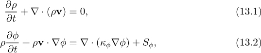
where φ is the scalar variable (e.g., υx, υy, υz, and enthalpy h, etc.), κφ is the “diffusion” coefficient associated with φ, and Sφ is usually called the source term in the φ equation, but actually it contains all other terms that do not fit into the given format.
Following the chain rule of differentiation, we have:
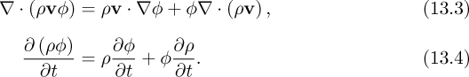
Thus, Eqn. (13.2) for φ can be rewritten as:

Note that the last two terms on the left-hand side are zero due to the mass conservation equation, Eqn. (13.1). It is customary to join the diffusion term with the convection term together on the left-hand side of the equation as follows:
The general convection/diffusion equation is now written in the strong conservation form (in which all spatial derivatives are expressed as divergence terms). We will see the benefit of using the conservation form shortly in the next few sections.
Discretization. The objective of any numerical methods is to reduce a given continuum problem (an infinite number of degrees of freedom (DOFs)) to a discrete problem (a finite number of DOFs). Generally, CFD methods use two levels of discretization or approximation, as follows:
1. Domain discretization (or grid generation): in this step, the spatial domain is subdivided into a number of smaller, regular, and connected “subregions” called cells or elements (collectively, the cells/elements are called a grid or a mesh). The distribution of the density of the cells should follow the physics of the flow closely, namely, the grid density should be finer where flow conditions change rapidly (large gradients), and it can be coarser where flow conditions are constant or change very gradually.
2. Equation discretization: the governing PDEs are converted into algebraic forms for each and every cell or element by various numerical methods. Details will be shown in the following sections.
The resulting system of algebraic equations is then solved numerically after the application of appropriate boundary and initial conditions (for steady-state problems, initial conditions are simply a set of guessed values to initiate the computation).
There exist many well-established ways for discretizing the PDEs, such as: finite-difference, finite-volume, finite-element, spectral-element, boundary-element methods, and so on, and there are still more variants even within each “family.” Because of its applicability to FlowLab we will focus on finite-volume methods, with briefer mentions of finite-difference and finite-element methods.
Finite-difference methods. Finite-difference methods (FDMs) first discretize the domain with a grid, then approximate each derivative in the governing PDE by using a corresponding truncated Taylor’s series expansion. We illustrate with the following two-dimensional diffusion equation (Poisson’s equation):
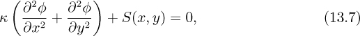
in which κ is a conductivity or diffusion coefficient and S is a source or generation term. The corresponding grid is shown in Fig. 13.1(a), with Fig. 13.1(b) showing a typical grid point P and its four neighbors, in which subscripts i and j denote positions in the x and y directions, and Δx and Δy are the corresponding grid spacings.
The Taylor’s series expansion for φ at the right-hand point (i +1, j) about its central value φi,j is:
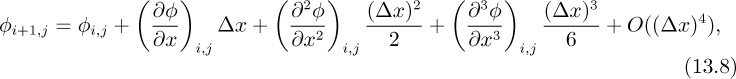
where we have used φi,j to represent φ(xi, yj), and O((Δx)4) indicates that the remaining terms in the expansion have a truncation error of order (Δx)4. Similarly:
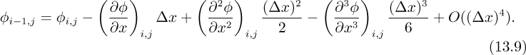
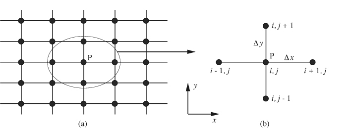
Fig. 13.1 (a) A simple two-dimensional finite-difference grid; (b) a representative point P and its four neighbors.
Addition of the last two equations and rearrangement gives us the centraldifference approximation for ∂2φ/∂x2 at (xi, yj):

with a similar approximation for ∂2φ/∂y2. Substitution of the difference approximations for the derivatives in Eqn. (13.7), and approximation of the source term S(xi, yj) by ![]() i,j (an averaged value in the vicinity of point P) gives:
i,j (an averaged value in the vicinity of point P) gives:

which is a discretized finite-difference form of the original differential equation.
Repetition of the procedure for each point in the two-dimensional grid yields a system of algebraic equations, which—after incorporating known values from the boundary conditions—has the same number of equations as the number of unknowns (the values of φi,j at the grid points, i = 1, 2,..., j = 1, 2,...). This set of equations can be solved for the unknowns φi,j by numerical methods developed for linear algebra.
The big advantage of the FDM is its simplicity. A major disadvantage is that for nonrectangular regions, especially with non-Dirichlet boundary conditions, special approximations have to be used to accommodate curved boundaries.
Finite-volume methods. In order to demonstrate the salient features of the finite-volume methods (FVM), we use a steady-state, convection-diffusion PDE in strong conservation form for illustration:
Without losing generality of the algorithm development, we will discretize the equation for a general two-dimensional mesh as shown in Fig. 13.2, in which the solution domain is subdivided into a finite number of nonoverlapping small control volumes, called cells. The computational nodes are placed at the centroid of each cell, in other words, all unknowns are stored in the cell centers. The starting point of the finite-volume methods is to use the integral form of the PDE with respect to each cell’s domain (Ω):

Fig. 13.2 A typical nonorthogonal two-dimensional finite-volume grid around a cell P and the notation used in the equation discretization.
Applying the Gauss divergence theorem in vector calculus, the volume integral on the left-hand side of Eqn. (13.13) becomes a surface integral over the boundary surface of the cell:
where n is the outward unit normal vector of the boundary surface S. For the sake of clarity, we separate the left-hand side integral of Eqn. (13.14) into two parts:

At this point, the advantage of the finite-volume formulation should become clear: it is inherently conservative because the strong conservation form provides for each cell or control volume a balance of fluxes across the cell’s boundary surface, just like we apply conservation laws to an open system.3
3 In contrast, a finite-difference formulation based on PDEs in nonconservation form may lead to numerical difficulties in situations where the dependent variables may be discontinuous, as in flows containing shocks.
Each finite-volume cell is bounded by a group of flat boundary surfaces, hence the surface integral can be expressed as the sum of integrals over all faces of the cell. Now the convective flux in Eqn. (13.15) can be treated as follows:

where Sf = nSf is the surface normal vector of face f. In Eqn. (13.16) we adopt the “midpoint rule” to calculate approximately the surface integral on a face by the inner product of the integrand evaluated at the centroid of the face and the face vector Sf. The midpoint rule can be shown to be second-order spatially accurate. The diffusive flux in Eqn. (13.15) can be treated similarly:
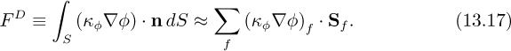
Both the convective and diffusive fluxes in Eqns. (13.16) and (13.17) require knowledge of solution variables and properties on the cell’s boundary faces, but in the cell-centered finite-volume formulation (see Fig. 13.2), all unknowns are stored in the cell centroids, e.g., φ, velocity components (υx, υy, υz), pressure (p) and physical properties (μ, ρ, k,...), etc. Hence we need to utilize some kind of interpolation or approximation techniques to evaluate the integrands on the cell faces in Eqns. (13.16) and (13.17) from the values at the cell centers. Many methods have been developed for this purpose, and here we illustrate the procedure with a general technique that can be used in any kind of mesh topology. First, we turn to the Taylor’s series expansion of φ in multiple dimensions:
where P denotes the centroid of a cell, and r is the position vector. In other words, it states that the following linear distribution of φ about P:
is second-order spatially accurate because the truncation error term scales with O(|(r – rP)2|). In order to use Eqn. (13.19), we need to know the gradient (∇φ)P at the centroid. The following vector calculus identity derived from the Gauss divergence theorem is very handy for that purpose:

By using the midpoint rule in Eqn. (13.20), the cell-centroid gradient can be calculated as

where VP is the cell’s volume. The value of φf at the boundary-face center can be linearly reconstructed by using Eqn. 13.19:
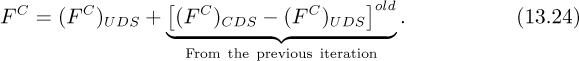
Now that the variables on each face of cell P are obtained, the convective flux FC in Eqn. (13.16) can be calculated (simple initializations and the iterative nature of the CFD solver will take care of the “circular relationship” between (∇φ)P and φf after just a few iterations). However, we need to point out that the linear reconstruction scheme outlined here belongs to the family of central-differencing scheme (CDS), which is known to cause the problem of spurious oscillations, or unboundedness, of the solution when the solution field changes rapidly in a region with a relatively coarse mesh. An alternative approach that guarantees boundedness is to determine φf according to direction of the flow approaching the face as follows:
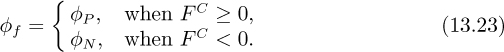
This is called the upwind differencing scheme (UDS). Unfortunately the boundedness of the UDS is secured at the expense of accuracy, since it is only first-order spatially accurate. In fact, the UDS scheme effectively introduces an excessive amount of “numerical diffusion” to the discretization of the convective terms. One trick to preserve the boundedness and accuracy simultaneously is to use a deferred correction scheme:
Another way is to adopt one of the bounded second-order upwind schemes, which will not be discussed here. Interested readers may refer to the references for details [3, 4, 11].
In order to calculate the diffusive flux FD, we need to obtain the gradient of φ at the cell face centers in Eqn. (13.17). For the face f of control volume P in Fig. 13.2, notice that the only contribution to the diffusive flux through f is from the derivative in the surface-normal direction (n):
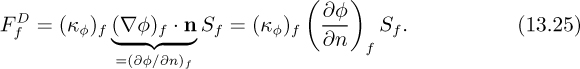
To represent (∂φ/∂n)f implicitly (i.e., by using the unknowns stored at the neighboring centroids), the derivative in Eqn. (13.25) is approximated by a central differencing scheme in the ξ direction (the direction of the line connecting centroids P and N), then correcting by the difference between the gradients in the ξ and n directions obtained explicitly from the previous (“old”) iteration:

where ![]() is the distance between P and N, and iξ is the unit vector along line
is the distance between P and N, and iξ is the unit vector along line ![]() . To obtain
. To obtain ![]() we may first use Eqn. (13.21) to calculate the cell-centered gradients at P and N, then interpolate to face f:
we may first use Eqn. (13.21) to calculate the cell-centered gradients at P and N, then interpolate to face f:

The approximation of the diffusive flux ![]() in Eqn. (13.26) is second-order accurate on uniform grids, free of potential un-physically oscillatory solutions, and applicable to arbitrary, nonorthogonal finite-volume meshes.
in Eqn. (13.26) is second-order accurate on uniform grids, free of potential un-physically oscillatory solutions, and applicable to arbitrary, nonorthogonal finite-volume meshes.
Finally, the discretization of the source term on the right-hand side of Eqn. (13.15) is carried out by first “linearizing” Sφ as:
where SU and SP are expressed in terms of constants and/or known values of field variables (possibly φ itself) based on the previous iteration. Then the volume integral of the source term is calculated as:
By substituting the discretized convection, diffusion, and source terms back into Eqn. (13.15), we can rewrite the discretization equation in the following format:
where the summation is over all neighboring cells (nb) sharing faces with cell P. In summary, the discretized equation quantitatively relates the unknown variables (φK) stored in neighboring cell centroids and sources to φP. When this procedure is repeated for each cell throughout the domain, and after appropriate boundary conditions are applied, we obtain a large system of algebraic equations, expressed as:
where A is the system matrix, b is the right-hand-side vector, and φ is the solution vector. This large, sparse system must be handled by iterative solution techniques. First, the so-called inner iterations start solving the linearized system by some iterative methods (for instance, Gauss-Seidel or the more advanced Krylov subspace methods) [4]. Then in the outer iterations the entries in A and b are updated so that the next round of inner iterations can work on an improved linearized system. This cycle is repeated until a converged result is obtained.
Within the limitations of space and scope in this chapter, we have managed to cover a central part of the finite-volume algorithm. For a complete treatment of the FVM, many topics—such as how to calculate the pressure and treat the pressure-velocity link (i.e., how to treat the continuity equation), and methods for unsteady problems, etc., need to be covered. But we will leave those topics for interested readers to pursue in the references [4, 12].
Finite-element methods. We again use the diffusion equation for a brief discussion of the finite-element method (FEM). At its simplest, as in Fig. 13.3(a), the region Ω is subdivided into a number of triangular elements interconnected at a total of n nodes. Note that by using varying sizes and orientations of elements, a curved boundary can be approximated fairly easily. As in Fig. 13.3(b), each node i has associated with it a shape or basis function ![]() that equals one at node i and declines linearly to zero at all the immediately adjacent nodes (and is zero beyond them).
that equals one at node i and declines linearly to zero at all the immediately adjacent nodes (and is zero beyond them).
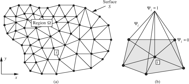
Fig. 13.3 (a) Subdivision of a region into triangular finite elements, (b) a typical node i and neighboring triangular elements, with a linear shape function![]() .
.
Let ![]() represent an approximate solution to the PDE of Eqn. (13.7). If φi denotes the value of
represent an approximate solution to the PDE of Eqn. (13.7). If φi denotes the value of ![]() at node i, the dependent variable
at node i, the dependent variable ![]() at any point is expressed by:
at any point is expressed by:

which amounts to representing ![]() over the whole region by linear interpolation of the nodal values φi.
over the whole region by linear interpolation of the nodal values φi.
Since ![]() is an approximate solution, it does not satisfy the differential equation exactly, there being a non-zero residual R when
is an approximate solution, it does not satisfy the differential equation exactly, there being a non-zero residual R when ![]() is substituted for φ:
is substituted for φ:

Note that the PDE of Eqn. (13.33) is more general than Eqn. (13.7) and allows for a spatial variation of κ—a feature that is easily accommodated by the FEM.
The next step employs the method of weighted residuals, in which the weighted integrals of R over the entire region Ω are set to zero, as expressed in the following n equations:
Here, the wj are n different weight functions, which—in line with the popular Galerkin method—are simply chosen to be the same as the shape functions, so that wj = ψj. The formidable-looking integral over the whole region Ω is greatly simplified because ψj is non-zero only in the immediate vicinity of node j, and the integral therefore reduces to summation of contributions from a mere handful of elements. The method essentially amounts to satisfying the PDE in an average way in n small subregions centered on each of the nodes.
The discretized equations for the Galerkin method are obtained from Eqn. (13.34) by substituting the shape function representation for ![]() from Eqn. (13.32). The integral of
from Eqn. (13.32). The integral of ![]() is further simplified by applying Green’s formula, which amounts to integration by parts in any number of space dimensions:
is further simplified by applying Green’s formula, which amounts to integration by parts in any number of space dimensions:

Eqn. (13.35) has two important merits:
1. It replaces a second-order derivative (![]() ) by the product of two first-order derivatives (∇ Ψi and
) by the product of two first-order derivatives (∇ Ψi and ![]() ), each of which just amounts to a constant because the shape functions are linear.
), each of which just amounts to a constant because the shape functions are linear.
2. It introduces the normal derivative of the dependent variable at the surface, which often appears in boundary conditions that involve a conductive or diffusive flux κ∂![]() /∂n of mass, energy, or momentum.
/∂n of mass, energy, or momentum.
Again we will get a large system of algebraic equations, Aφ = b, for which the coefficient matrix A is typically “banded,” and for which special solution techniques are available for the solution vector φ of nodal values φ1,φ2,...φn. Improved accuracy is obtained by using more elements and/or more sophisticated ones that involve quadratic or even higher-order shape functions. The above method is vertex-based, but element-based methods can also be applied, in which the weighted residual is set to zero for every element.
A major advantage of the FEM is that the mathematical properties of its algorithms are developed more rigorously than those of the FVM and FDM. For example, the convergence analysis and error estimates of the FEM algorithms can be shown to fit snugly into the framework of modern theory of differential equations [7]. A major disadvantage of the FEM for CFD is its substantially higher cost in CPU time and computer memory in comparison with the other two methods.
13.3. Learning CFD by Using FlowLab
The study of CFD for engineers should not end with theories only, it also needs to include practical examples in order to gradually build up the necessary problem-solving capabilities. In the remaining sections of this chapter, we will utilize FlowLab from Fluent Inc. to facilitate this process.
FlowLab is an educational CFD software package (based on the FVM) designed to be a virtual fluid laboratory using computers to conduct numerical experiments, in order to teach and enhance physical concepts in fluid mechanics and heat transfer. FlowLab provides an easy and friendly user interface so that users can start using CFD before acquiring more extensive knowledge in its theories and methodologies. It is available on the current Linux and Microsoft Windows platforms. Information regarding FlowLab’s software license, installation, documentation and support, etc. can be found at the website: http://flowlab.fluent.com
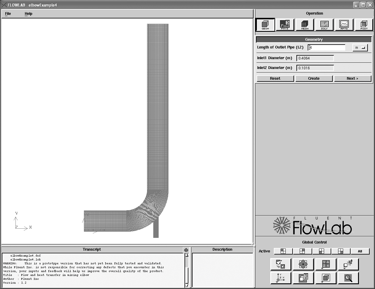
FlowLab structure. FlowLab is designed to integrate seamlessly a CFD preprocessor (to create the domain and generate a suitable mesh), a solver, and postprocessor (to visualize the solution and extract useful information from the vast amount of data) in a single graphical user interface (GUI). This is managed by using problem-specific template files. From the user’s viewpoint, FlowLab is built on top of a number of ready-to-use exercises,4 which are called templates created from the general-purpose CFD software FLUENT (solver and postprocessor) and its preprocessor called GAMBIT.5 A sample screen shot of the GUI is shown in Fig. 13.4.
4 New exercises are continuously created by FlowLab developers and users in academia. Available FlowLab exercises include flow over a Clark-Y airfoil, flow in an orifice meter, flow over a heated plate, flow over a cylinder, and a sudden expansion in a pipe, etc. A complete and up-to-date list is available at http://flowlab.fluent.com
5 FLUENT is a comprehensive finite-volume solver (for both structured and unstructured grids) for a widerange of flow modeling applications. See the website http://www.fluent.com for additional information about FLUENT.
How to use FlowLab. The following general steps will give you the general idea of using FlowLab to solve a problem in fluid mechanics.
1. When you start FlowLab, a launcher window will appear. Select Start a new session for a new problem, and highlight the template problem you want to work on, then click Start.
2. On the upper right portion of the FlowLab GUI, shown in Fig. 13.4, lies the Operation Toolpad, shown in Fig. 13.5. It consists of a series of command buttons, each of which is connected to the corresponding graphical panel. The layout of the buttons from left to right reflects the general order of operation when setting up a CFD problem: Geometry to define the problem domain, Physics to specify physical models, boundary conditions, and material properties, Mesh to create/refine mesh, Solve to start a CFD computation, Reports to analyze the computational results and generate x/y plots, and Postprocessing to create plots of contours, vectors, iso-surfaces, and particle tracks, etc.

3. A series of screen shots of the Operation Toolpad panels are presented below in order give you a visual overview of a typical FlowLab session (involving a developing pipe-flow problem):
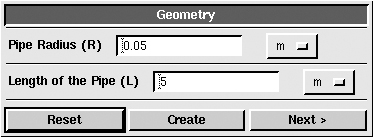
(a) Fig. 13.6 gives the Geometry panel for specifying the size and other geometrical features of the problem.
(b) Fig. 13.7 shows the panels for Physics, Boundary Condition, and Material properties. Users can freely specify the physical model (laminar or turbulent, with or without heat transfer), boundary condition, and material properties for each simulation so that it is a well-posed problem—in other words, all the model conditions should be physically consistent and correct. For example, one cannot expect FlowLab to generate correct results if the flow is specified as laminar while the Reynolds number is 106!

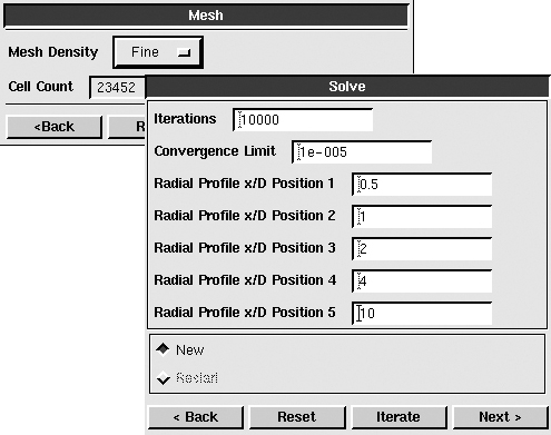
(c) Fig. 13.8 shows the Mesh and Solve panels. In the Mesh panel, you can select a mesh from various levels of fineness from the drop-down menu, click the generate button, and a grid will be generated and shown in the graphics window. You can use the mouse to examine the mesh more closely (drag the right button to zoom in or zoom out). In the Solve panel, you can set up the number of iterations, convergence limit (for the scaled residuals of the discretized equations), and also select the locations where you will be able to view profiles of solution variables after the computation is converged. Finally, click the iterate button, the solver will start the calculation, and an x/y plot of the residuals’ history will pop up and show the progress of the iteration process (the magnitudes of residuals should drop substantially before the calculation can be declared as a converged solution). After a while it will prompt you when the solution has converged. Now you can move on to the Postprocessing phase to view the results of the numerical model.
(d) Fig. 13.9 shows the Reports and Postprocessing panels, from where you can generate plots and visualize field data in many different ways, including animations.

4. Views and display attributes of the model can be easily manipulated by using Global Control buttons that are located in the lower right portion of the FlowLab GUI. A brief description of the function of each button is provided in the Description window (located in the lower center of the GUI) when the mouse cursor is placed on top of that button. Detailed description of the use of Global Control buttons can be found in the FlowLab User’s Guide.
5. Before studying the CFD examples in the next section, you should read the first three chapters of the FlowLab User’s Guide for an overview of the software package and its graphical user interface. A sample CFD session is also included in the documentation to guide you step by step from problem setup to examination of CFD results. You will quickly find out the FlowLab software is very easy to learn and use, so you can concentrate on the physics of the fluid dynamics problems.
13.4. Practical CFD Examples
In the remaining part of this chapter, we solve four example problems to introduce the basic features and limitations of CFD software. For a beginner, it is usually best to learn from simpler problems before trying to attack a more complicated one. In the following examples, we emphasize the proper understanding of the physics of each problem when setting up the case. After we have obtained a converged solution, we need to check the results very carefully in order to make sure the solution is either validated by experimental results or is physically reasonable. You are also encouraged to modify the setup of each case, including the sizes of the flow domain, mesh density, boundary conditions (BCs), and physical properties, etc. in order to build up your own hands-on experience.
Example 13.1—Developing Flow in a Pipe Entrance Region (FlowLab)
Problem Setup
We consider a steady-state, laminar developing flow (ReD= 300) in the pipe entrance region shown in Fig. E13.1.1.

The flow is steady, incompressible, and axisymmetric. The domain’s axial length is at least 50D (50 pipe diameters). The following key points should be taken into consideration while setting up the model:
• The flow is laminar when ReD < 2300.
• Because the gradient of velocity in the near-wall region is high, the mesh should be finer in the radial direction near the wall. We first select the “medium” mesh density and click on the Create button to establish a mesh for the computational domain.
• Inlet boundary condition: constant velocity at the inlet. (To make the setup process simple for FlowLab users, the following BCs are specified without requesting user’s input: Outlet: constant static pressure. Wall: no-slip. Axis of symmetry: axisymmetry.)
• Given a pipe diameter, for example, D = 0.1 m (caution: in FlowLab you specify the radius, not the diameter, during the setup of the problem), and length L is 5 m so that L/D = 50. In order to ensure that the Reynolds number of the flow is 300, one can pick any fluid (so the kinematic viscosity ν is fixed), then calculate the corresponding inlet velocity. For example, a fluid with ρ = 1 kg/m3 and μ = 10–6 kg/m s, we need to set ![]() = 0.003 m/s for ReD = 300.
= 0.003 m/s for ReD = 300.
• The mesh (“medium” mesh density) created by FlowLab is shown in Fig. E13.1.2. In this particular mesh there are 6,678 two-dimensional rectangular cells. For calculating the flow, three equations (mass conservation, x- and y-momentum equations) are needed for each cell, so in total 20,034 simultaneous equations are solved numerically. If heat transfer is also calculated (using the energy equation), another 6,678 equations would be added to the system.

Fig. E13.1.2 An enlarged view of the finite-volume mesh used in the developing flow calculation in FlowLab Example 13.1. It is only shown partially due to the high aspect ratio of the domain.
Results and Discussion
• The axial length of the pipe entrance region, called the hydrodynamic entrance length Le, can be shown to scale with D ReD by using the integral boundary-layer method [13]:
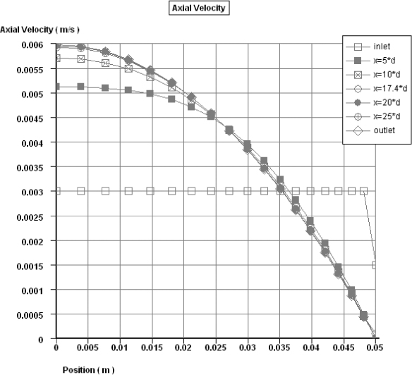
For ReD = 300, we get Le/D ≈ 17.4. In order to verify this result, we can use FlowLab’s convenient x/y plot tool to plot the axial velocity profiles along several axial locations. As shown in Fig. E13.1.3, the velocity profiles (at x/D = 0, 5, and 10) are still developing before x/D = 17.4. Beyond this point, e.g., at x/D = 20, 25, and 30, all profiles become identical and collapse into a single curve in the figure.
• For a fully developed laminar pipe flow, the static pressure should vary linearly along the axial direction (in other words, dp/dx is constant). The plot of static pressure versus the axial distance (x) from our FlowLab calculation verifies this point. You can see pressure variation is closely linear in the fully developed region (Le > 0.174 m) in Fig. E13.1.4.

Fig. E13.1.4 Static pressure distribution in the axial direction for a developing laminar pipe flow (ReD = 300, D = 0.1 m).
• You can also plot the wall friction factor f along the axis. The hydrodynamic entrance length Le is also defined as the distance required for the friction factor to reach within 5% of its fully developed value. For laminar flow, f = 64/ReD. Use the plot to verify the CFD results.
• Thermal entrance length (Leth): Perform the heat transfer calculation of this developing flow problem by enabling the energy equation for the model in the Physics panel and go through the iterations until convergence. Then plot the wall Nusselt number Nu along the axial direction. The thermal entrance length is defined as the distance from the pipe inlet required for the Nusselt number to reach within 5% of its fully developed value Nu∞ (for instance, Nu = 4.364 for a constant heat-flux wall). Examine the relationship between the thermal entrance length and the hydrodynamic entrance length Le for different Prandtl numbers (Pr).
• Grid independence (effect of the grid resolution): Compute the same flow with the coarse and fine mesh densities, then compare the predicted results of the entrance length among the different grids. Verify that the laminar flow entrance length predicted by FlowLab is not affected by the grid resolution.
Example 13.2—Pipe Flow Through a Sudden Expansion (FlowLab)
Problem Setup
Flow through a sudden expansion such as that in Fig. E13.2.1 occurs frequently in a piping system. Here we study an axisymmetric case of such a flow.

The problem is set up according to the following considerations:
• The flow is assumed to be incompressible—an assumption that is valid for almost all liquids, and for gases when the fluid speed is less than 30% of the local speed of sound.
• The inlet pipe length L1 should be at least ten times the inlet pipe radius R1. The length L2 should be 50 times the step size (R2 – R1) or longer. A domain configured as such allows reasonably accurate specifications of the inlet and outlet boundary conditions detailed below. (These are very conservative ratios—you may shorten the outlet and inlet lengths without appreciably changing the numerical results.)
• Based on the inlet pipe diameter, the flow is laminar when Re < 1,000. At a higher Reynolds number, the flow is in the turbulent regime and needs to be modeled by a suitable turbulence model. Here we use the standard k-ε two-equation model [8]. For an excellent review of eddy-viscosity turbulence models, see [2].
• Inlet boundary condition: constant velocity normal to the inlet. To make the problem setup process simple for FlowLab users, the following BCs are specified without requesting user’s input. Inlet: k and ε are specified via the turbulence intensity and a turbulence length scale. Outlet: constant static pressure. Axis: axisymmetry. Wall: no-slip.
• In order to resolve steep gradients, the mesh needs to be very fine near the wall. We also need a fine mesh for the regions above and below the imaginary line extending downstream from the corner of the step, because there exists a boundary-free shear-layer structure (i.e., with large gradients) beyond the step’s corner.6
6 This is a good example of applying basic understanding in fluid mechanics when running CFD. The need for a fine mesh in the shear-layer structure is not as obvious as the requirement in the near-wall region, but it is critical for obtaining accurate numerical results.
• For a sample calculation, take R1 = 0.1 m, R2 = 0.2 m, L1 = 1m, L2 = 5m. Use standard air properties (the default in FlowLab) for the fluid. At the inlet, the velocity ![]() = 1.34 m/s is given, and the Reynolds number (based on the inlet pipe diameter) for this case is 20,000. Finally, use the “coarse” mesh density and turbulence model’s enhanced wall treatment (designated Enh-wall in FlowLab) for the wall boundary.7
= 1.34 m/s is given, and the Reynolds number (based on the inlet pipe diameter) for this case is 20,000. Finally, use the “coarse” mesh density and turbulence model’s enhanced wall treatment (designated Enh-wall in FlowLab) for the wall boundary.7
7 Enhanced wall treatment is to use an advanced two-layer zonal model for the near-wall region combined with a blending wall function for the complete turbulent boundary layer including viscous sublayer, buffer layer, log-law layer and outer layer [5].
Taking all the points above into account, we can properly set up the governing equations, geometry, fluid properties, boundary conditions, and mesh for the problem in FlowLab.
Results and Discussion
• We can use the postprocessing tools of FlowLab to visualize the computed results. For example, the streamline plot of Fig. E13.2.2 provides us the visualization of the flow separation and reattachment zone behind the step. You can use the tools to plot velocity vectors, contours, and more.
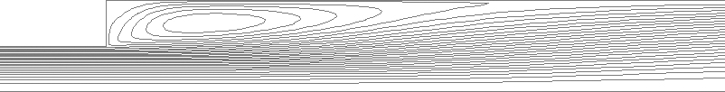
Fig. E13.2.2 Streamline plot for the recirculation zone in a pipe’s sudden expansion: Re = 20,000 (based on the inlet pipe diameter), expansion ratio R2/R1 = 2.
• For calculating the head loss generated by a pipe expansion, we can evaluate the discharge coefficient K of the sudden expansion, which is defined as:

where “1” is at the expansion point and “2” is at the reattachment point of the separation. For the current sample calculation (R2/R1= 2), FlowLab reports K = 0.549. The discharge coefficient for other expansion ratios can be quickly obtained by changing the expansion ratio (we may still fix R1 = 0.1 m, and Re = 20,000), re-generating the domain and the mesh, then running the CFD calculations. For example, using the coarse mesh option, a few computed versus theoretical values of K [13] are given in Table E13.2.1.

• Grid independence: You can run these same cases with different mesh densities and compare the results with theoretical values.
• Many other interesting features of this problem can be examined by using FlowLab. For example: predictions of the re-attachment point, the centerline velocity and pressure distributions, skin friction factor at the wall downstream of the step, and centerline total pressure distribution, etc.
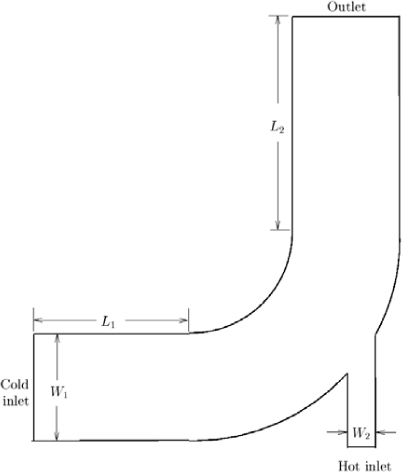
Example 13.3—A Two-Dimensional Mixing Junction (FlowLab)
Problem Setup
This example studies two-dimensional turbulent flow in the channel junction of Fig. E13.3.1. The cold fluid coming into the main channel from the left (inlet 1) is mixed with the same fluid at a higher temperature from a smaller side channel at the corner (inlet 2). We will use this example to investigate the complex flow mixing patterns and the effect of velocity and temperature on the mixing results.
• The flow is incompressible and turbulent (one should check the Reynolds number to confirm that this is the case). Since we are interested in the convection heat transfer of the mixing flow, we need to enable the heat transfer calculation in the Physics panel.
• The outlet section length L2 is adjustable by the user. Note that when changing the inlet velocities (especially the velocity of the hot stream), it is possible to cause a flow recirculation zone in the main channel. If that happens, the outlet section length must be long enough in order to get an accurate numerical result. The point is to make sure that the outlet plane is not cutting through the recirculation zone. This requirement is quite common in all CFD simulation, it is due to the fact that general boundary conditions at outlets do not work well when significant backflow occurs.
• Inlet boundary conditions: constant fluid velocity and temperature are specified at the respective inlets. (To make the setup simple for FlowLab users, the following BCs are specified without requesting user’s input. Wall: no slip and adiabatic (zero heat flux). Outlet: constant pressure.)
• Users must exercise caution and make sure the Reynolds number based on the hydraulic diameter DH of the main channel (DH1 = 2W1) is high enough for the flow to be turbulent. The standard two-equation k-ε turbulence model is used in this example, together with “Std-wall” (standard wall-function—the logarithmic law of the wall) as the wall BC.
• A case under investigation can be set up as follows: Geometry: outlet length L2 = 4 m, cold-inlet width W1 = 0.4064 m, hot-inlet width W2 = 0.1016 m; fluid property ν = 10–6 m2/s, mesh: medium density; BCs: T1 = 293 K, ![]() 1 = 0.492126 m/s,
1 = 0.492126 m/s, ![]() = 1 m/s, and T2 = 313 K. The resulting main inlet Reynolds number Re1 is 400,000. A second case with identical setup except for a different hot-inlet velocity (
= 1 m/s, and T2 = 313 K. The resulting main inlet Reynolds number Re1 is 400,000. A second case with identical setup except for a different hot-inlet velocity (![]() ) will be used later for the study of flow separation pattern in the mixing junction.
) will be used later for the study of flow separation pattern in the mixing junction.
Results and Discussion
• Streamline and temperature contours for two different flow conditions are shown in Fig. E13.3.2 and Fig. E13.3.3, respectively. The two cases have the same cold-inlet velocity (hence the Reynolds number Re1), but have different velocities at the hot-stream (small) inlet. The streamline contours in Fig. E13.3.2 indicate that the resulting flow patterns are very different between the two. When the ratio of hot-inlet to the cold-inlet velocities ![]() is 4, no separation occurs at the mixing junction; but when the ratio is 10 a sizable separation and recirculation zone appears. The flow pattern affects very strongly the mixing of the cold and hot streams, as illustrated by the temperature contours shown in Fig. E13.3.3.
is 4, no separation occurs at the mixing junction; but when the ratio is 10 a sizable separation and recirculation zone appears. The flow pattern affects very strongly the mixing of the cold and hot streams, as illustrated by the temperature contours shown in Fig. E13.3.3.
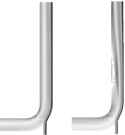
Fig. E13.3.2 Streamline patterns of the two-dimensional mixing junction flows: all conditions are the same for both cases except that the hot-inlet velocity on the right is 2.5 times higher than that of the case on the left. The higher hot-inlet velocity gives rise to a sizable separation/recirculation zone downstream of the junction.

Fig. E13.3.3 Temperature contours of the two-dimensional mixing junction flows: all conditions are the same for both cases except that the hot-inlet velocity on the right is 2.5 times higher than that of the case on the left. Due to the presence of a sizable separation/recirculation zone for the case on the right, the temperature distribution of the mixing junction is drastically different than that of the case on the left, which has no separation zone.
• This example serves to illustrate an advantage of CFD in many industrial applications: numerical simulations provide excellent quantitative results for engineering design and analysis. For example, it is almost impossible to predict the flow patterns (with or without separation) under different inlet velocities in the mixing junction by either physical intuition or by using basic principles in fluid mechanics without the knowledge of complete velocity and pressure fields of the flow.
• The standard k-ε turbulence model is known to be very dissipative; in other words, the high turbulent viscosity in the recirculation region tends to “damp out” vortices. Therefore when the standard k-ε model predicts separation, it is indeed likely to be the case. But additional validations should be conducted to support this conclusion.
• A cautionary statement should be given here about turbulence models and CFD: although numerous turbulence models have been developed over the last twenty some years, there is not yet a single turbulence model that can reliably predict all turbulent flows in industrial applications with sufficient accuracy.8 You may find the previous statement very disappointing or even depressing, but the state of our lack of understanding of the essential physics of turbulence was succinctly summarized by Richard P. Feynman (Nobel Laureate in Physics, 1965)—turbulence is “the most important unresolved problem of classical physics.” Surely we do need turbulence modeling for CFD (so it is very important to know the strengths and weaknesses of turbulence models), but we—as CFD practitioners—also need to examine very carefully the results and conduct further validations, for instance, by comparing CFD predictions with experimental data, or with other similar flow data published in the literature, etc. before jumping to a conclusion.
8 Yet proponents of a particular turbulence model might want you to think otherwise.
Example 13.4—Flow Over a Cylinder (FlowLab)
Problem Setup
Consider the flow in Fig. E13.4.1 about a circular cylinder of diameter D immersed in a steady cross flow of velocity U∞ (the uniform undisturbed stream velocity). One might guess the flow to be perfectly steady, but, depending on the Reynolds number, it is actually oscillatory. When ReD = ρU∞D/μ > 40, the flow becomes unsteady and regularly sheds an array of alternating vortices from the cylinder. The flow pattern is called a Kármán vortex street, named after Theodore von Kármán, who provided a theoretical analysis of this phenomenon in 1912.

This is a fundamental fluid mechanics problem of practical importance. We will use this example to examine the predicted drag coefficient, the vortex-shedding frequency of the flow, and the beautiful flow patterns.
• The flow is modeled as a two-dimensional flow over a circle. The flow domain is created as follows: diameter of the cylinder is 0.1 m, the upstream distance is 5 times the diameter, and downstream distance is 25 times the diameter. Width of the domain is 25 times the diameter.
• The flow is laminar if ReD < 1,000. The FlowLab template for flow over a cylinder is designed to work well in the range 1 < ReD< 1,000. Here we set ReD = 100 (say, ρ = 1 kg/m3, μ = 10–5 kg/m s with U∞= 0.01 m/s), so that the case lies in the range for the laminar, incompressible, and vortex-shedding flow.
• Boundary condition: constant velocity U∞ = 0.01 m/s at the inlet (on the left). To make the setup simple for FlowLab users, the following BCs are specified without requesting user input. Cylinder wall: no-slip. Outlet (on the right): constant pressure. Top and bottom boundaries: periodic (which means that solutions along the pair of boundaries are completely identical).
• Initial condition: the following initial condition is given without requesting user input: uniform u = υx = 0.01 m/s; in order to break the symmetry of the flow and “trigger” the vortex shedding, a very small perturbation is applied to the flow by initially setting v = υy = 0.00005 m/s.
• Select “medium” mesh and click Generate button in the Mesh panel. An enlarged view of the finite-volume mesh in the vicinity of the cylinder is shown in Fig. E13.4.2. The quality of the mesh near the cylinder’s surface and in the wake of the cylinder is very critical. This mesh has a total of 16,176 quadrilateral cells in the solution domain.

Fig. E13.4.2 An enlarged view of the finite-volume mesh in the vicinity of the cylinder in the cross flow.
• Starting from a uniform flow approaching the cylinder from the left-hand side, this unsteady-flow case requires a substantial amount of computing time in order to observe counterrotating vortices to develop and then move downstream. Make sure the time-step size (Δt) is not too large (we use a “conservative” Δt = 1 s to resolve the fluctuations in the time domain) and that the iterations have sufficiently converged during each time step before advancing to the next time step. You can also specify how often (in terms of the flow time) the field data set are saved for visualizing the flow at the postprocessing stage.
• For this current case (medium mesh density, Δt = 1 s), it takes about 80 minutes of wall clock time to simulate 1,000 time-steps (i.e., 1,000 seconds of flow time) on an IBM PC workstation (2.8 GHz Pentium 4 CPU,2 GB of RAM, Windows XP operating system).
Results and Discussion
• The vortex-shedding frequency n is often expressed as a non-dimensional quantity called the Strouhal number S:
In the range 40 < S < 104, the Strouhal number depends uniquely on the Reynolds number ReD. We can use FlowLab’s postprocessing feature (a point object) to monitor the time history, e.g., the y velocity history at x = 0.7 m in the wake region, shown in Fig. E13.4.3, then derive the frequency of the oscillations from it. The frequency n is simply the inverse of the period, which is 64 seconds measured in the figure between two adjacent peaks. With U∞ = 0.01 m/s and D = 0.1 m, the Strouhal number S calculated by FlowLab is 0.156, which is within 5% of the experimental value of 0.165 ± 0.08 [10].

• The drag coefficient of the cylinder is defined as:
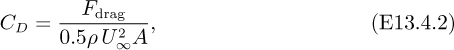
where A is the frontal area as seen from the approaching stream. For a two-dimensional cylinder in a cross flow, A = D × 1 (a unit depth perpendicular to the plane). FlowLab calculations predict CD = 1.33. The reported experimental values of CD at ReD = 100 have quite a wide variation in the literature, ranging from 1.26 [1], 1.41 [6], 1.46 [9] to 1.6 [10]. The discrepancy is possibly due to the three-dimensional effects or fluctuations of the free stream in the wind tunnel. The numerical prediction given by FlowLab falls right within the range of the data and is considered to be quite satisfactory.
• Figs. E13.4.4 and E13.4.5 show a series of velocity-magnitude contour plots of the cylinder flow, from the initial symmetric flow pattern to the final regular shedding of alternating vortices. The flow is quite symmetric initially (t < 50 s); at around 200 s, the tail end of the wake has started to flap. The pattern of alternating vortices shed from the cylinder is increasingly clear at 250 s, and the Kármán vortex street has reached its regular (periodic) stage at t = 400 s. In FlowLab you can easily generate animations to view such unsteady flow patterns.

Fig. E13.4.4 Velocity contour plots of the flow over a cylinder (ReD= 100), at t = 50 s (top) and t = 200 s (bottom) from the beginning of the simulation. At t = 200 s, the tail end of the wake has started to flap and the initial symmetry (as seen at t = 50 s) of the flow has been destroyed.

Fig. E13.4.5 (Continued from Fig. E13.4.4) Velocity contour plots at t = 250 s (top) and t = 400 s (bottom). After being shed from the cylinder, the vortices move alternately clockwise (top row) and counterclockwise (bottom row). The Kármán vortex street is already regularly periodic at the later time.
Summary. In the previous FlowLab examples we have demonstrated that CFD can do a very good job in flows with well-understood physics (e.g., incompressible, steady or unsteady, laminar flow), if and when users provide a well-posed problem with a sufficient mesh resolution and with proper boundary/initial conditions. When the flow is turbulent and/or is more involved in terms of complex physics (e.g., multiple phases, chemical reactions, etc., which are beyond the scope of this chapter), users should exercise extra caution in properly selecting turbulence and additional physical models, and critically examine the CFD results to avoid possible blunders in trusting blindly those “seemingly reasonable” predictions.
References for Chapter 13
1. G.K. Batchelor, An Introduction to Fluid Dynamics, Cambridge University Press, 1967, p. 261.
2. J. Bredberg, “On two-equation eddy-viscosity models,” Internal Report 01/8, Dept. of Thermodynamics and Fluid Dynamics, Chalmers University of Technology, Göteborg, Sweden, 2001.
3. C.-Y. Cheng, E.A. Lim, D. Fee, T.M. Foster, H.S. Kunanayagam and P.R. Tuladhar, “Comparisons of higher-order differencing schemes in a two dimensional, incompressible finite-volume scalar transport code,” Joint ASME and JSME Fluids Engineering Conference, Hilton Head, SC, August 13–18, 1995.
4. J.H. Ferziger and M. Perić, Computational Methods for Fluid Dynamics, Springer Verlag, 2nd ed., 1999.
5. Fluent Incorporated, FLUENT 6.1 User’s Guide, 2003.
6. S. Hoerner, Fluid-Dynamic Drag, Hoerner Fluid Dynamics, Bakersfield, CA, 1965.
7. A. Iserles, A First Course in the Numerical Analysis of Differential Equations, Cambridge University Press, Cambridge, 1996.
8. B.E. Launder and D.B. Spalding, Lectures in Mathematical Models of Turbulence, Academic Press, London, 1972.
9. A.F. Mills, Basic Heat and Mass Transfer, Richard D. Irwin, Inc., Chicago, 1995, p. 251.
10. H. Schlichting, Boundary-Layer Theory, 7th ed., McGraw-Hill, New York, 1968.
11. J.C. Tannehill, D.A. Anderson, and R.H. Pletcher, Computational Fluid Mechanics and Heat Transfer, 2nd ed., Taylor & Francis, Washington DC, 1997.
12. H. Versteeg and W. Malalasekra, Introduction to Computational Fluid Dynamics: The Finite-Volume Approach, Prentice-Hall, Upper Saddle River, NJ, 1996.
13. F.M. White, Fluid Mechanics, 4th ed., McGraw-Hill, New York, 1999.