
Chapter 17
Using Graphics Hardware
Peter Willemsen
17.1 Hardware Overview
Throughout most of this book, the focus is on the fundamentals that underly computer graphics rather than on any specifics relating to the APIs or hardware on which the algorithms may be implemented. This chapter takes a slightly different route and blends the details of using graphics hardware with some of the practical issues associated with programming that hardware. The chapter is designed to be an introductory guide to graphics hardware and could be used as the basis for a set of weekly labs that investigate graphics hardware.
17.2 What Is Graphics Hardware
Graphics hardware describes the hardware components necessary to quickly render 3D objects as pixels on your computer’s screen using specialized rasterization-based (and in some cases, ray-tracer–based) hardware architectures. The use of the term graphics hardware is meant to elicit a sense of the physical components necessary for performing a range of graphics computations. In other words, the hardware is the set of chipsets, transistors, buses, processors, and computing cores found on current video cards. As you will learn in this chapter, and eventually experience yourself, current graphics hardware is very good at processing descriptions of 3D objects and transforming those representations into the colored pixels that fill your monitor.
Graphics hardware has certainly changed very rapidly over the last decade. Newer graphics hardware provides more parallel processing capabilities, as well as better support for specialized rendering. One explanation for the fast pace is the video game industry and its economic momentum. Essentially what this means is that each new graphics card provides better performance and processing capabilities. As a result, video games appear more visually realistic. The processors on graphics hardware, often called GPUs, or Graphics Processing Units, are highly parallel and afford thousands of concurrent threads of execution. The hardware is designed for throughput which allows larger numbers of pixels and vertices to be processed in shorter amounts of time. All of this parallelism is good for graphics algorithms, but other work has benefited from the parallel hardware. In addition to video games, GPUs are used to accelerate physics computations, develop real-time ray tracing codes, solve Navier-Stokes related equations for fluid flow simulations, and develop faster codes for understanding the climate (Purcell, Buck, Mark, & Hanrahan, 2002; S. G. Parker et al., 2010; Harris, 2004). Several APIs and SDKs have been developed that afford more direct general purpose computation, such as OpenCL and NVIDIA’s CUDA. Hardware accelerated ray tracing APIs also exist to accelerate ray-object intersection (S. G. Parker et al., 2010). Similarly, the standard APIs that are used to program the graphics components of video games, such as OpenGL and DirectX, also allow mechanisms to leverage the graphics hardware’s parallel capabilities. Many of these APIs change as new hardware is developed to support more sophisticated computations.
Graphics hardware is programmable. As a developer, you have control over much of the computations associated with processing geometry, vertices, and the fragments that eventually become pixels. Recent hardware changes as well as ongoing updates to the APIs, such as OpenGL or DirectX, support a completely programmable pipeline. These changes afford developers creative license to exploit the computation available on GPUs. Prior to this, fixed-function rasterization pipelines forced the computation to a specific style of vertex transformations, lighting, and fragment processing. The fixed functionality of the pipeline ensured that basic coloring, lighting, and texturing could occur very quickly. Whether it is a programmable interface, or fixed-function computation, the basic computations of the rasterization pipeline are similar, and follow the illustration in Figure 17.1. In the rasterization pipeline, vertices are transformed from local space to global space, and eventually into screen coordinates, after being transformed by the viewing and projection transformation matrices. The set of screen coordinates associated with a geometry’s vertices are rasterized into fragments. The final stages of the pipeline process the fragments into pixels and can apply per-fragment texture lookups, lighting, and any necessary blending. In general, the pipeline lends itself to parallel execution and the GPU cores can be used to process both vertices and fragments concurrently. Additional details about the rasterization pipeline can be found in Chapter 8.
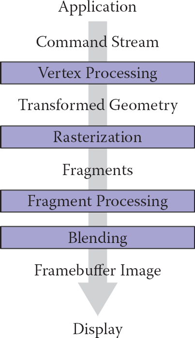
The basic graphics hardware pipeline consists of stages that transform 3D data into 2D screen objects ready for rasterizing and coloring by the pixel processing stages.
17.3 Heterogeneous Multiprocessing
When using graphics hardware, it is convenient to distinquish between the CPU and the GPU as separate computational entities. In this context, the term host is used to refer to the CPU including the threads and memory available to it. The term device is used to refer to the GPU, or the graphics processing units, and the threads and memory associated with it. This makes some sense because most graphics hardware is comprised of external hardware that is connected to the machine via the PCI bus. The hardware may also be soldered to the machine as a separate chipset. In this sense, the graphics hardware represents a specialized co-processor since both the CPU (and its cores) can be programmed, as can the GPU and its cores. All programs that utilize graphics hardware must first establish a mapping between the CPU and the GPU memory. This is a rather low-level detail that is necessary so that the graphics hardware driver residing within the operating system can interface between the hardware and the operating system and windowing system software. Recall that because the host (CPU) and the device (GPU) are separate, data must be communicated between the two systems. More formally, this mapping between the operating system, the hardware driver, the hardware, and the windowing system is known as the graphics context. The context is usually established through API calls to the windowing system. Details about establishing a context is outside the scope of this chapter, but many windowing system development libraries have ways to query the graphics hardware for various capabilities and establish the graphics context based on those requirements. Because setting up the context is windowing system dependent, it also means that such code is not likely to be cross-platform code. However, in practice, or at least when starting out, it is very unlikely that such low-level context setup code will be required since many higher level APIs exist to help people develop portable interactive applications.
Many of the frameworks for developing interactive applications support querying input devices such as the keyboard or mouse. Some frameworks provide access to the network, audio system, and other higher level system resources. In this regard, many of these APIs are the preferred way to develop graphics, and even game applications.
Cross-platform hardware acceleration is often achieved with the OpenGL API. OpenGL is an open industry standard graphics API that supports hardware acceleration on many types of graphics hardware. OpenGL represents one of the most common APIs for programming graphics hardware along with APIs such as DirectX. While OpenGL is available on many operating systems and hardware architectures, DirectX is specific to Microsoft-based systems. For the purposes of this chapter, hardware programming concepts and examples will be presented with OpenGL.
17.3.1 Programming with OpenGL
When you program with the OpenGL API, you are writing code for at least two processors: the CPU(s) and the GPU(s). OpenGL is implemented in a C-style API and all functions are prefixed with “gl” to indicate their inclusion with OpenGL. OpenGL function calls change the state of the graphics hardware and can be used to declare and define geometry, load vertex and fragment shaders, and determine how computation will occur as data passes through the hardware.
The variant of OpenGL that this chapter presents is the OpenGL 3.3 Core Profile version. While not the most recent version of OpenGL, the 3.3 version of OpenGL is in line with the future direction of OpenGL programming. These versions are focused on improving efficiency while also fully placing the programming of the pipeline within the hands of the developer. Many of the function calls present in earlier versions of OpenGL are not present in these newer APIs. For instance, immediate mode rendering is deprecated. Immediate mode rendering was used to send data from the CPU memory to the graphics card memory as needed each frame and was often very inefficient, especially for larger models and complex scenes. The current API focuses on storing data on the graphics card before it is needed and instancing it at render time. As another example, OpenGL’s matrix stacks have been deprecated as well, leaving the developer to use third-party matrix libraries (such as GLM) or their own classes to create the necessary matrices for viewing, projection, and transformation, as presented in Chapter 7. As a result, OpenGL’s shader language (GLSL) has taken on larger roles as well, performing the necessary matrix tranformations along with lighting and shading within the shaders. Because the fixed-function pipeline which performed per-vertex transformation and lighting is no longer present, programmers must develop all shaders themselves. The shading examples presented in this chapter will utilize the GLSL 3.3 Core Profile version shader specification. Future readers of this chapter will want to explore the current OpenGL and OpenGL Shading Language specifications for additional details on what these APIs and languages can support.
17.4 Graphics Hardware Programming: Buffers, State, and Shaders
Three concepts will help to understand contemporary graphics hardware programming. The first is the notion of a data buffer, which is quite simply, a linear allocation of memory on the device that can store various data on which the GPUs will operate. The second is the idea that the graphics card maintains a computational state that determines how computations associated with scene data and shaders will occur on the graphics hardware. Moreover, state can be communicated from the host to the device and even within the device between shaders. Shaders represent the mechanism by which computation occurs on the GPU related to per-vertex or per-fragment processing. This chapter will focus on vertex and fragment shaders, but specialized geometry and compute shaders also exist in the current versions of OpenGL. Shaders play a very important role in how modern graphics hardware functions.
17.4.1 Buffers
Buffers are the primary structure to store data on graphics hardware. They represent the graphics hardware’s internal memory associated with everything from geometry, textures, and image plane data. With regard to the rasterization pipeline described in Chapter 8, the computations associated with hardware-accelerated rasterization read and write the various buffers on the GPU. From a programming standpoint, an application must initialize the buffers on the GPU that are needed for the application. This amounts to a host to device copy operation. At the end of various stages of execution, device to host copies can be performed as well to pull data from the GPU to the CPU memory. Additionally, mechanisms do exist in OpenGL’s API that allow device memory to be mapped into host memory so that an application program can write directly to the buffers on the graphics card.
17.4.2 Display Buffer
In the graphics pipeline, the final set of pixel colors can be linked to the display, or they may be written to disk as a PNG image. The data associated with these pixels is generally a 2D array of color values. The data is inherently 2D, but it is efficiently represented on the GPU as a 1D linear array of memory. This array implements the display buffer, which eventually gets mapped to the window. Rendering images involves communicating the changes to the display buffer on the graphics hardware through the graphics API. At the end of the rasterization pipeline, the fragment processing and blending stages write data to the output display buffer memory. Meanwhile, the windowing system reads the contents of the display buffer to produce the raster images on the monitor’s window.
17.4.3 Cycle of Refresh
Most applications prefer a double-buffered display state. What this means is that there are two buffers associated with a graphics window: the front buffer and the back buffer. The purpose of the double-buffered system is that the application can communicate changes to the back buffer (and thus, write changes to that buffer) while the front-buffer memory is used to drive the pixel colors on the window.
At the end of the rendering loop, the buffers are swapped through a pointer exchange. The front-buffer pointer points to the back buffer and the back-buffer pointer is then assigned to the previous front buffer. In this way, the windowing system will refresh the content of the window with the most up-to-date buffer. If the buffer pointer swap is synchronized with the windowing system’s refresh of the entire display, the rendering will appear seamless. Otherwise, users may observe a tearing of the geometry on the actual display as changes to the scene’s geometry and fragments are processed (and thus written to the display buffer) faster than the screen is refreshed.
When the display is considered a memory buffer, one of the simplest operations on the display is essentially a memory setting (or copying) operation that zeros-out, or clears the memory to a default state. For a graphics program, this likely means clearing the background of the window to a specific color. To clear the background color (to black) in an OpenGL application, the following code can be used:
glClearColor(0.0f, 0.0f, 0.0f, 1.0f);
glClear(GL_COLOR_BUFFER_BIT);
The first three arguments for the glClearColor function represent the red, green, and blue color components, specified within the range [0, 1]. The fourth argument represents opacity, or alpha value, ranging from 0.0 being completely transparent to 1.0 being completely opaque. The alpha value is used to determine transparency through various fragment blending operations in the final stages of the pipeline.
This operation only clears the color buffer. In addition to the color buffer, specified by GL_COLOR_BUFFER_BIT, being cleared to black in this case, graphics hardware also uses a depth buffer to represent the distance that fragments are relative to the camera (you may recall the discussion of the z-buffer algorithm in Chapter 8). Clearing the depth buffer is necessary to ensure operation of the z-buffer algorithm and allow correct hidden surface removal to occur. Clearing the depth buffer can be achieved by or’ing two bit field values together, as follows:
glClear(GL_COLOR_BUFFER_BIT | GL_DEPTH_BUFFER_BIT);
Within a basic interactive graphics application, this step of clearing is normally the first operation performed before any geometry or fragments are processed.
17.5 State Machine
By illustrating the buffer-clearing operation for the display’s color and depth buffers, the idea of graphics hardware state is also introduced. The glClearColor function sets the default color values that are written to all the pixels within the color buffer when glClear is called. The clear call initializes the color component of the display buffer and can also reset the values of the depth buffer. If the clear color does not change within an application, the clear color need only be set once, and often this is done in the initialization of an OpenGL program. Each time that glClear is called it uses the previously set state of the clear color.
Note also that the z-buffer algorithm state can be enabled and disabled as needed. The z-buffer algorithm is also known in OpenGL as the depth test. By enabling it, a fragment’s depth value will be compared to the depth value currently stored in the depth buffer prior to writing any fragment colors to the color buffer. Sometimes, the depth test is not necessary and could potentially slow down an application. Disabling the depth test will prevent the z-buffer computation and change the behavior of the executable. Enabling the z-buffer test with OpenGL is done as follows:
glEnable(GL_DEPTH_TEST);
glDepthFunc(GL_LESS);
The glEnable call turns on the depth test while the glDepthFunc call sets the mechanism for how the depth comparison is performed. In this case, the depth function is set to its default value of GL_LESS to show that other state variables exist and can be modified. The converse of the glEnable calls are glDisable calls.
The idea of state in OpenGL mimics the use of static variables in object-oriented classes. As needed, programmers enable, disable, and/or set the state of OpenGL variables that reside on the graphics card. These state then affect any succeeding computations on the hardware. In general, efficient OpenGL programs attempt to minimize state changes, enabling states that are needed, while disabling states that are not required for rendering.
17.6 Basic OpenGL Application Layout
A simple and basic OpenGL application has, at its heart, a display loop that is called either as fast as possible, or at a rate that coincides with the refresh rate of the monitor or display device. The example loop below uses the GLFW library, which supports OpenGL coding across multiple platforms.
while (!glfwWindowShouldClose(window)) {
{
// OpenGL code is called here,
// each time this loop is executed.
glClear(GL_COLOR_BUFFER_BIT | GL_DEPTH_BUFFER_BIT);
// Swap front and back buffers
glfwSwapBuffers(window);
// Poll for events
glfwPollEvents() ;
if (glfwGetKey(window, GLFW_KEY_ESCAPE) == GLFW_PRESS)
glfwSetWindowShouldClose(window, 1);
}
The loop is tightly constrained to operate only while the window is open. This example loop resets the color buffer values and also resets the z-buffer depth values in the graphics hardware memory based on previously set (or default) values. Input devices, such as keyboards, mouse, network, or some other interaction mechanism are processed at the end of the loop to change the state of data structures associated with the program. The call to glfwSwapBuffers synchronizes the graphics context with the display refresh, performing the pointer swap between the front and back buffers so that the updated graphics state is displayed on the user’s screen. The call to swap the buffers occurs after all graphics calls have been issued.
While conceptually separate, the depth and color buffers are often collectively called the framebuffer. By clearing the contents of the framebuffer, the application can proceed with additional OpenGL calls to push geometry and fragments through the graphics pipeline. The framebuffer is directly related to the size of the window that has been opened to contain the graphics context. The window, or viewport, dimensions are needed by OpenGL to construct the Mvp matrix (from Chapter 7) within the hardware. This is accomplished through the following code, demonstrated again with the GLFW toolkit, which provides functions for querying the requested window (or framebuffer) dimensions:
int nx, ny;
glfwGetFramebufferSize(window, &nx, &ny);
glViewport(0, 0, nx, ny);
In this example, glViewport sets the OpenGL state for the window dimension using nx and ny for the width and height of the window and the viewport being specified to start at the origin.
Technically, OpenGL writes to the framebuffer memory as a result of operations that rasterize geometry, and process fragments. These writes happen before the pixels are displayed on the user’s monitor.
17.7 Geometry
Similar to the idea of a display buffer, geometry is also specified using arrays to store vertex data and other vertex attributes, such as vertex colors, normals, or texture coordinates needed for shading. The concept of buffers will be used to allocate storage on the graphics hardware, transferring data from the host to the device.
17.7.1 Describing Geometry for the Hardware
One of the challenges with graphics hardware programming is the management of the 3D data and its transfer to and from the memory of the graphics hardware. Most graphics hardware work with specific sets of geometric primitives. The different primitive types leverage primitive complexity for processing speed on the graphics hardware. Simpler primitives can sometimes be processed very fast. The caveat is that the primitive types need to be general purpose so as to model a wide range of geometry from very simple to very complex. On typical graphics hardware, the primitive types are limited to one or more of the following:
- points—single vertices used to represent points or particle systems;
- lines—pairs of vertices used to represent lines, silhouettes, or edge-highlighting;
- triangles—triangles, triangle strips, indexed triangles, indexed triangle strips, quadrilaterals, or triangle meshes approximating geometric surfaces.
These three primitive types form the basic building blocks for most geometry that can be defined. An example of a triangle mesh rendered with OpenGL is shown in Figure 17.2.
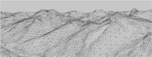
How your geometry is organized will affect the performance of your application. This wireframe depiction of the Little Cottonwood Canyon terrain dataset shows tens of thousands of triangles organized as a triangle mesh running at real-time rates.
The image is rendered using the VTerrain Project terrain system courtesy of Ben Discoe.
17.8 A First Look at Shaders
Modern versions of OpenGL require that shaders be used to process vertices and fragments. As such, no primitives can be rendered without at least one vertex shader to process the incoming primitive vertices and another shader to process the rasterized fragments. Advanced shader types exist within OpenGL and the OpenGL Shading Language: geometry shaders and compute shaders. Geometry shaders are designed to process primitives, potentially creating additional primitives, and can support geometric instancing operations. Compute shaders are designed for performing general computation on the GPU, and can be linked into the set of shaders necessary for a specific application. For more information on geometry and compute shaders, the reader is referred the OpenGL specification documents and other resources.
17.8.1 Vertex Shader Example
Vertex shaders provide control over how vertices are transformed and often help prepare data for use in fragment shaders. In addition to standard transformations and potential per-vertex lighting operations, vertex shaders could be used to perform general computation on the GPU. For instance, if the vertices represent particles and the particle motion can be (simply) modeled within the vertex shader computations, the CPU can mostly be removed from performing those computations. The ability to perform computations on the vertices already stored in the graphics hardware memory is a potential performance gain. While this approach is useful in some situations, advanced general computation may be more appropriately coded with compute shaders.
In Chapter 7, the viewport matrix Mvp was introduced. It transforms the canonical view volume coordinates to screen coordinates. Within the canonical view volume, coordinates exist in the range of [−1, 1]. Anything outside of this range is clipped. If we make an initial assumption that the geometry exists within this range and the z-value is ignored, we can create a very simple vertex shader. This vertex shader passes the vertex positions through to the rasterization stage, where the final viewport transformation will occur. Note that because of this simplification, there are no projection, viewing, or model transforms that will be applied to the incoming vertices. This is initially cumbersome for creating anything except very simple scenes, but will help introduce the concepts of shaders and allow you to render an initial triangle to the screen. The passthrough vertex shader follows:
#version 330 core
layout (location=0) in vec3 in_Position;
void main(void)
{
gl_Position = vec4(in_Position, 1.0);
}
This vertex shader does only one thing. It passes the incoming vertex position out as the gl_Position that OpenGL uses to rasterize fragments. Note that gl_Position is a built-in, reserved variable that signifies one of the key outputs required from a vertex shader. Also note the version string in the first line. In this case, the string instructs the GLSL compiler that version 3.3 of the GLSL Core profile is to be used to compile the shading language.
Vertex and fragment shaders are SIMD operations that respectively operate on all the vertices or fragments being processed in the pipeline. Additional data can be communicated from the host to the shaders executing on the device by using input, output, or uniform variables. Data that is passed into a shader is prefixed with the keyword in. The location of that data as it relates to specific vertex attributes or fragment output indices is also specified directly in the shader. Thus,
layout(location=0) in vec3 in_Position;
specifies that in_Position is an input variable that is of type vec3. The source of that data is the attribute index 0 that is associated with the geometry. The name of this variable is determined by the programmer, and the link between the incoming geometry and the shader occurs while setting up the vertex data on the device. The GLSL contains a nice variety of types useful to graphics programs, including vec2, vec3, vec4, mat2, mat3, and mat4 to name a few. Standard types such as int or float also exist. In shader programming, vectors, such as vec4 hold 4-components corresponding to the x, y, z, and w components of a homogeneous coordinate, or the r, g, b, and a components of a RGBA tuple. The labels for the types can be interchanged as needed (and even repeated) in what is called swizzling (e.g., in_Position.zyxa). Moreover, the component-wise labels are overloaded and can be used appropriately to provide context.
All shaders must have a main function that performs the primary computation across all inputs. In this example, the main function simply copies the input vertex position (in_Position), which is of type vec3 into the built-in vertex shader output variable, which is of type vec4. Note that many of the built-in types have constructors that are useful for conversions such as the one presented here to convert the incoming vertex position’s vec3 type into gl_Position’s vec4 type. Homogeneous coordinates are used with OpenGL, so 1.0 is specified as the fourth coordinate to indicate that the vector is a position.
17.8.2 Fragment Shader Example
If the simplest vertex shader simply passes clip coordinates through, the simplest fragment shader sets the color of the fragment to a constant value.
#version 330 core
layout(location=0) out vec4 out_FragmentColor;
void main(void)
{
out_FragmentColor = vec4(0.49, 0.87, 0.59, 1.0);
}
In this example, all fragments will be set to a light shade of green. One key difference is the use of the out keyword. In general, the keywords in and out in shader programs indicate the flow of data into, and out of, shaders. While the vertex shader received incoming vertices and output them to a built-in variable, the fragment shader declares its outgoing value which is written out to the color buffer:
layout(location=0) out vec4 out_FragmentColor;
The output variable out_FragmentColor is again user defined. The location of the output is color buffer index 0. Fragment shaders can output to multiple buffers, but this is an advanced topic left to the reader that will be needed if OpenGL’s framebuffer objects are investigated. The use of the layout and location keywords makes an explicit connection between the application’s geometric data in the vertex shader and the output color buffers in the fragment shader.
17.8.3 Loading, Compiling, and Using Shaders
Shader programs are transferred onto the graphics hardware in the form of character strings. They must then be compiled and linked. Furthermore, shaders are coupled together into shader programs so that vertex and fragment processing occur in a consistent manner. A developer can activate a shader that has been successfully compiled and linked into a shader program as needed, while also deactivating shaders when not required. While the detailed process of creating, loading, compiling, and linking shader programs is not provided in this chapter, the following OpenGL functions will be helpful in creating shaders:
- glCreateShader creates a handle to a shader on the hardware.
- glShaderSource loads the character strings into the graphics hardware memory.
- glCompileShader performs the actual compilation of the shader within the hardware.
The functions above need to be called for each shader. So, for the simple pass-through shaders, each of those functions would be called for both the vertex shader code and the fragment shader code provided. At the end of the compilation phase, compilation status and any errors can be queried using additional OpenGL commands.
After both shader codes are loaded and compiled, they can be linked into a shader program. The shader program is what is used to affect rendering of geometry.
- glCreateProgram creates a program object that will contain the previously compiled shaders.
- glAttachShader attaches a shader to the shader program object. In the simple example, this function will be called for both the compiled vertex shader and the compiled fragment shader objects.
- glLinkProgram links the shaders internally after all shaders have been attached to the program object.
- glUseProgram binds the shader program for use on the graphics hardware. As shaders are needed, the program handles are bound using this function. When no shaders are needed, they can be unbound by using the shader program handle 0 as an argument to this function.
17.9 Vertex Buffer Objects
Vertices are stored on the graphics hardware using buffers, known as vertex buffer objects. In addition to vertices, any additional vertex attributes, such as colors, normal vectors, or texture coordinates, will also be specified using vertex buffer objects.
First, let’s focus on specifying the geometric primitive themselves. This starts by allocating the vertices associated with the primitive within the host memory of the application. The most general way to do this is to define an array on the host to contain the vertices needed for the primitive. For instance, a single triangle, fully contained within the canonical volume, could be defined statically on the host as follows:
GLfloat vertices[] = {-0.5f, -0.5f, 0.0f, 0.5f, -0.5f, 0.0f, 0.0f, 0.5f, 0.0f};
If the simple passthrough shaders are used for this triangle, then all vertices will be rendered. Although the triangle is placed on the z = 0 plane, the z coordinates for this example do not really matter since they are essentially dropped in the final transformation into screen coordinates. Another thing to note is the use of the type GLfloat in these examples. Just as the GLSL language has specialized types, OpenGL has related type which generally can intermix well with the standard types (like float). For preciseness, the OpenGL types will be used when necessary.
Before the vertices can be processed, a vertex buffer is first created on the device to store the vertices. The vertices on the host are then transferred to the device. After this, the vertex buffer can be referenced as needed to draw the array of vertices stored in the buffer. Moreover, after the initial transfer of vertex data, no additional copying of data across the host to device bus need occur, especially if the geometry remains static across rendering loop updates. Any host memory can also be deleted if it was dynamically allocated.
Vertex buffer objects, often called VBOs, represent the primary mechanism with modern OpenGL to store vertex and vertex attributes in the graphics memory. For efficiency purposes, the initial setup of a VBO and the transfer of vertex-related data mostly happens prior to entering the display loop. As an example, to create a VBO for this triangle, the following code could be used:
GLuint triangleVBO[1];
glGenBuffers(1, triangleVBO);
glBindBuffer(GL_ARRAY_BUFFER, triangleVBO[0]);
glBufferData(GL_ARRAY_BUFFER, 9 * sizeof(GLfloat), vertices, GL_STATIC_DRAW);
glBindBuffer(GL_ARRAY_BUFFER, 0);
Three OpenGL calls are required to create and allocate the vertex buffer object. The first, glGenBuffers creates a handle that can be used to refer to the VBO once it is stored on the device. Multiple handles to VBOs (stored in arrays) can be created in a single glGenBuffers call, as illustrated but not utilized here. Note that when a buffer object is generated, the actual allocation of space on the device is not yet performed.
With OpenGL, objects, such as vertex buffer objects, are primary targets for computation and processing. Objects must be bound to a known OpenGL state when used and unbound when not in use. Examples of OpenGL’s use of objects include the vertex buffer objects, framebuffer objects, texture objects, and shader programs, to name a few. In the current example, the GL_ARRAY_BUFFER state of OpenGL is bound to the triangle VBO handle that was generated previously. This essentially makes the triangle VBO the active vertex buffer object. Any operations that affect vertex buffers that follow the glBindBuffer(GL_ARRAY_BUFFER, triangleVBO[0]) command will use the triangle data in the VBO either by reading the data or writing to it.
Vertex data is copied from the host (the vertices array) to the device (currently bound GL_ARRAY_BUFFER) using the
glBufferData(GL_ARRAY_BUFFER, 9 * sizeof(GLfloat), vertices, GL_STATIC_DRAW);
call. The arguments represent the type of target, the size in bytes of the buffer to be copied, the pointer to the host buffer, and an enumerated type that indicates how the buffer will be used. In the current example, the target is GL_ARRAY_BUFFER, the size of the data is 9* sizeof(GLfloat), and the last argument is GL_STATIC_DRAW indicating to OpenGL that the vertices will not change over the course of the rendering. Finally, when the VBO no longer needs to be an active target for reading or writing, it is unbound with the glBindBuffer(GL_ARRAY _BUFFER, 0) call. In general, binding any of OpenGL’s objects or buffers to handle 0, unbinds, or disables that buffer from affecting subsequent functionality.
17.10 Vertex Array Objects
While vertex buffer objects are the storage containers for vertices (and vertex attributes), vertex array objects represent OpenGL’s mechanism to bundle vertex buffers together into a consistent vertex state that can be communicated and linked with shaders in the graphics hardware. Recall that the fixed function pipeline of the past no longer exists and therefore, per-vertex state, such as normals or even vertex colors, must be stored in hardware buffers and then referenced in shaders, using input variables (e.g., in).
As with vertex buffer objects, vertex array objects, or VAOs, must be created and allocated with any necessary state being set while the vertex array object is bound. For instance, the following code shows how to create a VAO to contain the triangle VBO previously defined:
GLuint VAO;
glGenVertexArrays(1, &VAO);
glBindVertexArray(VAO);
glEnableVertexAttribArray(0);
glBindBuffer(GL_ARRAY_BUFFER, triangleVBO[0]);
glVertexAttribPointer(0, 3, GL_FLOAT, GL_FALSE, 3 * sizeof(GLfloat), 0);
glBindVertexArray(0);
When defining a vertex array object, specific vertex buffer objects can be bound to specific vertex attributes (or inputs) in shader code. Recall the use of
layout(location=0) in vec3 in_Position
in the passthrough vertex shader. This syntax indicate that the shader variable will receive its data from attribute index 0 in the bound vertex array object. In host code, the mapping is created using the
glEnableVertexAttribArray(0);
glBindBuffer(GL_ARRAY_BUFFER, triangleVBO[0]);
glVertexAttribPointer(0, 3, GL_FLOAT, GL_FALSE, 3 * sizeof(GLfloat), 0);
calls. The first call enables the vertex attribute index (in this case, 0). The next two calls connect the previously defined vertex buffer object that holds the vertices to the vertex attribute itself. Because glVertexAttribPointer utilizes the currently bound VBO, it is important that the glBindBuffer is issued before assigning the vertex attribute pointer. These function calls create a mapping that binds the vertices in our vertex buffer to the in_Position variable within the vertex shader. The glVertexAttribPointer calls seems complicated but it basically sets attribute index 0 to hold three components (e.g., x, y, z) of GLfloats (the 2nd and 3rd arguments) that are not normalized (the fourth argument). The fifth argument instructs OpenGL that three float values separate the starts of each vertex set. In other words, the vertices are tightly packed in the memory, one after the other. The final argument is a pointer to the data, but because a vertex buffer has been bound prior to this call, the data will be associated with the vertex buffer.
The previous steps that initialize and construct the vertex array object, the vertex buffer objects, and the shaders should all be executed prior to entering the display loop. All memory from the vertex buffer will have been transferred to the GPU and the vertex array objects will make the connection between the data and shader input variable indexes. In the display loop, the following calls will trigger the processing of the vertex array object:
glBindVertexArray(VAO);
glDrawArrays(GL_TRIANGLES, 0, 3);
glBindVertexArray(0);
Note again, that a bind call makes the vertex array object active. The call to glDrawArrays initiates the pipeline for this geometry, describing that the geometry should be interpreted as a series of triangle primitives starting at offset 0 and only rendering three of the indices. In this example, there are only three elements in the array and the primitive is a triangle, so a single triangle will be rendered.
Combining all of these steps, the assembled code for the triangle would resemble the following, assuming that shader and vertex data loading are contained in external functions:
// Set the viewport once
int nx, ny;
glfwGetFramebufferSize(window, &nx, &ny);
glViewport(0, 0, nx, ny);
// Set clear color state
glClearColor(0.0f, 0.0f, 0.0f, 1.0f) ;
// Create the Shader programs, VBO, and VAO
GLuint shaderID = loadPassthroughShader();
GLuint VAO = loadVertexData();
while (!glfwWindowShouldClose(window)) {
{
glClear(GL_COLOR_BUFFER_BIT | GL_DEPTH_BUFFER_BIT);
glUseProgram(shaderID);
glBindVertexArray(VAO);
glDrawArrays(GL_TRIANGLES, 0, 3);
glBindVertexArray(0);
glUseProgram(0);
// Swap front and back buffers
glfwSwapBuffers(window);
// Poll for events
glfwPollEvents() ;
if (glfwGetKey(window, GLFW_KEY_ESCAPE) == GLFW_PRESS)
glfwSetWindowShouldClose(window, 1);
}
Figure 17.3 shows the result of using the shaders and vertex state to render the canonical view volume triangle.

17.11 Transformation Matrices
Current versions of OpenGL have removed the matrix stacks that were once used to reference the projection and modelview matrices from the hardware. Because these matrix stacks no longer exist, the programmer must write matrix code that can be transferred to vertex shaders where the transformations will occur. That initially may seem challenging. However, several libraries and toolkits have been developed to assist with cross-platform development of OpenGL code. One of these libraries, GLM, or OpenGL Mathematics, has been developed to track the OpenGL and GLSL specifications closely so that interoperation between GLM and the hardware will work seamlessly.
17.11.1 GLM
GLM provides several basic math types useful to computer graphics. For our purposes, we will focus on just a few types and a handful of functions that make use of matrix transforms within the shaders easy. A few types that will be used include the following:
- glm::vec3—a compact array of 3 floats that can be accessed using the same component-wise access found in the shaders;
- glm::vec4—a compact array of 4 floats that can be accessed using the same component-wise access found in the shaders;
- glm::mat4—a 4 × 4 matrix storage represented as 16 floats. The matrix is stored in column-major format.
Similarly, GLM provides functions for creating the projection matrices, Morth and Mp, as well as functions for generating the view matrix, Mcam:
- glm::ortho creates a 4 × 4 orthographic projection matrix.
- glm::perspective creates the 4 × 4 perspective matrix.
- glm::lookAt creates the 4 × 4 homogeneous transform that translates and orients the camera.
17.11.2 Using an Orthographic Projection
A simple extension to the previous example would be to place the triangle vertices into a more flexible coordinate system and render the scene using an orthographic projection. The vertices in the previous example could become:
GLfloat vertices[] = {-3.0f, -3.0f, 0.0f, 3.0f, -3.0f, 0.0f, 0.0f, 3.0f, 0.0f};
Using GLM, an orthographic projection can be created easily on the host. For instance,
glm::mat4 projMatrix = glm::ortho(-5.0f, 5.0f, -5.0, 5.0, -10.0f, 10.0f);
The projection matrix can then be applied to each vertex transforming it into clip coordinates. The vertex shader will be modified to perform this operation:
This computation will occur in a modified vertex shader that uses uniform variables to communicate data from the host to the device. Uniform variables represent static data that is invariant across the execution of a shader program. The data is the same for all elements and remains static. However, uniform variables can be modified by an application between executions of a shader. This is the primary mechanism that data within the host application can communicate changes to shader computations. Uniform data often represent the graphics state associated with an application. For instance, the projection, view, or model matrices can be set and accessed through uniform variables. Information about light sources within a scene may also be obtained through uniform variables.
Modifying the vertex shader requires adding a uniform variable to hold the projection matrix. We can use GLSL’s mat4 type to store this data. The projection matrix can then be used naturally to tranform the incoming vertices into the canonical coordinate system:
#version 330 core
layout (location=0) in vec3 in_Position;
uniform mat4 projMatrix;
void main(void)
{
gl_Position = projMatrix * vec4(in_Position, 1.0);
}
The application code need only transfer the uniform variable from the host memory (a GLM mat4) into the device’s shader program (a GLSL mat4). This is easy enough, but requires that the host side of the application acquire a handle to the uniform variable after the shader program has been linked. For instance, to obtain a handle to the projMatrix variable, the following call would be issued once, after shader program linking is complete:
GLint pMatID = glGetUniformLocation(shaderProgram, "projMatrix");
The first argument is the shader program object handle and the second argument is the character string of the variable name in the shader. The id can then be used with a variety of OpenGL glUniform function call to transfer the memory on the host into the device. However, shader programs must first be bound prior to setting the value related to a uniform variable. Also, because GLM is used to store the projection matrix on the host, a GLM helper function will be used to obtain a pointer to the underlying matrix, and allow the copy to proceed.
glUseProgram(shaderID);
glUniformMatrix4fv(pMatID, 1, GL_FALSE, glm::value_ptr(projMatrix));
glBindVertexArray(VAO);
glDrawArrays(GL_TRIANGLES, 0, 3);
glBindVertexArray(0);
glUseProgram(0);
Notice the form that glUniform takes. The function name ends with characters that help define how it is used. In this case, a single 4 × 4 matrix of floats is being tranferred into the uniform variable. The v indicates that an array contains the data, rather than passing by value. The third argument lets OpenGL know whether the matrix should be transposed (a potentially handy feature), and the last argument is a pointer to the memory where the matrix resides.
By this section of the chapter, you should have a sense for the role that shaders and vertex data play in rendering objects with OpenGL. Shaders, in particular, form a very important role in modern OpenGL. The remaining sections will further explore the role of shaders in rendering scenes, atempting to build upon the role that shaders play in other rendering styles presented in this book.
17.12 Shading with Per-Vertex Attributes
The previous examples specified a single triangle with no additional data. Vertex attributes, such as normal vectors, texture coordinates, or even colors, can be interleaved with the vertex data in a vertex buffer. The memory layout is straightforward. Below, the color of each vertex is set after each vertex in the array. Three components are used to represent the red, green, and blue channels. Allocating the vertex buffer is identical with the exception being that the size of the array is now 18 GLfloats instead of 9.
GLfloat vertexData[] = {0.0f, 3.0f, 0.0f, 1.0f, 1.0f, 0.0f, -3.0f,
-3.0f, 0.0f, 0.0f, 1.0f, 1.0f, 3.0f, -3.0f, 0.0f, 1.0f, 0.0f, 1.0f};
The vertex array object specification is different. Because the color data is interleaved between vertices, the vertex attribute pointers must stride across the data appropriately. The second vertex attribute index must also be enabled. Building off the previous examples, we construct the new VAO as follows:
glBindBuffer(GL_ARRAY_BUFFER, m_triangleVBO[0]);
glEnableVertexAttribArray(0);
glVertexAttribPointer(0, 3, GL_FLOAT, GL_FALSE, 6 * sizeof(GLfloat), 0);
glEnableVertexAttribArray(1);
glVertexAttribPointer(1, 3, GL_FLOAT, GL_FALSE, 6 * sizeof(GLfloat), (const GLvoid *)12);
A single VBO is used and bound prior to setting the attributes since both vertex and color data are contained within the VBO. The first vertex attribute is enabled at index 0, which will represent the vertices in the shader. Note that the stride (the 5th argument) is different as the vertices are separated by six floats (e.g., the x, y, z of the vertex followed by the r, g, b of the color). The second vertex attribute index is enabled and will represent the vertex color attributes in the shader at location 1. It has the same stride, but the last argument now represents the pointer offset for the start of the first color value. While 12 is used in the above example, this is identical to stating 3 * sizeof(GLfloat). In other words, we need to jump across the three floats representing the vertex x, y, z values to locate the first color attribute in the array.
The shaders for this example are only slightly modified. The primary differences in the vertex shader (shown below) are (1) the second attribute, color, is at location 1 and (2) vColor is an output variable that is set in the main body of the vertex shader.
#version 330 core
layout (location=0) in vec3 in_Position;
layout (location=1) in vec3 in_Color;
out vec3 vColor;
uniform mat4 projMatrix;
void main(void)
{
vColor = in_Color;
gl_Position = projMatrix * vec4(in_Position, 1.0);
}
Recall that the keywords in and out refer to the flow of data between shaders. Data that flows out of the vertex shader becomes input data in the connected fragment shader, provided that the variable names match up. Moreover, out variables that are passed to fragment shaders are interpolated across the fragments using barycentric interpolation. Some modification of the interpolation can be achieved with additional keywords, but this detail will be left to the reader. In this example, three vertices are specified, each with a specific color value. Within the fragment shader, the colors will be interpolated across the face of the triangle.
The fragment shader changes are simple. The vColor variable that was set and passed out of the vertex shader now becomes an in variable. As fragments are processed, the vColor vec3 will contain the correctly interpolated values based on the location of the fragment within the triangle.
#version 330 core
layout(location=0) out vec4 fragmentColor;
in vec3 vColor;
void main(void)
{
fragmentColor = vec4(vColor, 1.0);
}
The image that results from running this shader with the triangle data is shown in Figure 17.4.

Setting the colors of each vertex in the vertex shader and passing the data to the fragment shader results in barycentric interpolation of the colors.
17.12.1 Structs of Vertex Data
The previous example illustrates the interleaving of data in an array. Vertex buffers can be used in a variety of ways, including separate vertex buffers for different model attributes. Interleaving data has advantages as the attributes associated with a vertex are near the vertex in memory and can likely take advantage of memory locality when operating in the shaders. While the use of these interleaved arrays is straightforward, it can become cumbersome to manage large models in this way, especially as data structures are used for building robust (and sustainable) software infrastructure for graphics (see Chapter 12). It is rather simple to store vertex data as vectors of structs that contain the vertex and any related attributes. When done this way, the structure need only be mapped into the vertex buffer. For instance, the following structure contains the vertex position and vertex color, using GLM’s vec3 type:
struct vertexData
{
glm::vec3 pos;
glm::vec3 color;
};
std::vector< vertexData > modelData;
The STL vector will hold all vertices related to all the triangles in the model. We will continue to use the same layout for triangles as in previous examples, which is a basic triangle strip. Every three vertices represents a triangle in the list. There are other data organizations that can be used with OpenGL, and Chapter 12 presents other options for organizing data more efficiently.
Once the data is loaded into the vector, the same calls used before load the data into the vertex buffer object:
int numBytes = modelData.size() * sizeof(vertexData);
glBufferData(GL_ARRAY_BUFFER, numBytes, modelData.data(), GL_STATIC_DRAW);
glBindBuffer(GL_ARRAY_BUFFER, 0);
STL vectors store data contiguously. The vertexData struct used above is represented by a flat memory layout (it does not contain pointers to other data elements) and is contiguous. However, the STL vector is an abstraction and the pointer that references the underlying memory must be queried using the data() member. That pointer is provided to the call to glBufferData. Attribute assignment in the vertex array object is identical as the locality of the vertex attributes remains the same.
17.13 Shading in the Fragment Processor
The graphics pipeline chapter (Chapter 8) and the surface shading chapter (Chapter 10) do a nice job of describing and illustrating the effects of per-vertex and per-fragment shading as they relate to rasterization and shading in general. With modern graphics hardware, applying shading algorithms in the fragment processor produces better visual results and more accurately approximates lighting. Shading that is computed on a per-vertex basis is often subject to visual artifacts related to the underlying geometry tessellation. In particular, per-vertex based shading often fails to approximate the appropriate intensities across the face of the triangle since the lighting is only being calculated at each vertex. For example, when the distance to the light source is small, as compared with the size of the face being shaded, the illumination on the face will be incorrect. Figure 17.5 illustrates this situation. The center of the triangle will not be illuminated brightly, despite being very close to the light source, since the lighting on the vertices, which are far from the light source, are used to interpolate the shading across the face. Of course, increasing the tessellation of the geometry can improve the visuals. However, this solution is of limited use in real-time graphics as the added geometry required for more accurate illumination can result in slower rendering.

Fragment shaders operate on the fragments that emerge from rasterization after vertices have been transformed and clipped. Generally speaking, fragment shaders must output a value that is written to a framebuffer. Often times, this is the color of the pixel. If the depth test is enabled, the fragment’s depth value will be used to control whether the color and its depth are written to the framebuffer memory. The data that fragment shaders use for computation comes from various sources:
- Built-in OpenGL variables. These variables are provided by the system. Examples of fragment shader variables include gl_FragCoord or gl_FrontFacing. These variables can change based on revisions to OpenGL and GLSL, so it is advised that you check the specification for the version of OpenGL and GLSL that you are targeting.
- Uniform variables. Uniform variables are transferred from the host to the device and can change as needed based on user input or changing simulation state in the application. These variables are declared and defined by the programmer for use within both vertex and fragment shaders. The projection matrix in the previous vertex shader examples was communicated to the shader via a uniform variable. If needed, the same uniform variable names can be used within both vertex and fragment shaders.
- Input variables. Input variables are specified in the fragment shader with the prefixed keyword in. Recall that data can flow into and out of shaders. Vertex shaders can output data to the next shader stage using the out keyword (e.g., out vec3 vColor, in a previous example). The outputs are linked to inputs when the next stage uses an in keyword followed by the same type and name qualifiers (e.g., in vec3 vColor in the previous example’s corresponding fragment shader).
Any data that is passed to a fragment shader through the in-out linking mechanism will vary on a per-fragment basis using barycentric interpolation. The interpolation is computed outside of the shader by the graphics hardware. Within this infrastructure, fragment shaders can be used to perform per-fragment shading algorithms that evaluate specific equations across the face of the triangle. Vertex shaders provide support computations, transforming vertices and staging intermediate per-vertex values that will be interpolated for the fragment code.
The following shader program code implements per-fragment, Blinn-Phong shading. It brings together much of what has been presented in this chapter thus far and binds it to the shader descriptions from Chapter 4. An interleaved vertex buffer is used to contain the vertex position and normal vectors. These values manifest in the vertex shader as vertex array attributes for index 0 and index 1. The shading computations that occur in the fragment shader code are performed in camera coordinates (sometimes referred to as eye-space).
17.13.1 Blinn-Phong Shader Program: Vertex Shader
The vertex shader stage of our program is used to transform the incoming vertices using the Mmodel and Mcam matrices into camera coordinates. It also uses the normal matrix, (M−1)T, to appropriately transform the incoming normal vector attribute. The vertex shader outputs three variables to the fragment stage:
- normal. The vertex’s normal vector as transformed into the camera coordinate system.
- h. The half-vector needed for Blinn-Phong shading.
- l. The light direction transformed into the camera coordinate system.
Each of these variables will then be available for fragment computation, after applying barycentric interpolation across the three vertices in the triangle.
A single point light is used with this shader program. The light position and intensity is communicated to both the vertex and fragment shaders using a uniform variable. The light data is declared using GLSL’s struct qualifer, which allows variables to be grouped together in meaningful ways. Although not presented here, GLSL supports arrays and for-loop control structures, so additional lights could easily be added to this example.
All matrices are also provided to the vertex shader using uniform variables. For now, we will imagine that the model (or local transform) matrix will be set to the indentity matrix. In the following section, more detail will be provided to expand on how the model matrix can be specified on the host using GLM.
#version 330 core
//
// Blinn-Phong Vertex Shader
//
layout(location=0) in vec3 in_Position;
layout(location=1) in vec3 in_Normal;
out vec4 normal;
out vec3 half;
out vec3 lightdir;
struct LightData {
vec3 position;
vec3 intensity;
};
uniform LightData light;
uniform mat4 projMatrix;
uniform mat4 viewMatrix;
uniform mat4 modelMatrix;
uniform mat4 normalMatrix;
void main(void)
{
// Calculate lighting in eye space: transform the local
// position to world and then camera coordinates.
vec4 pos = viewMatrix * modelMatrix * vec4(in_Position, 1.0);
vec4 lightPos = viewMatrix * vec4(light.position, 1.0);
normal = normalMatrix * vec4(in_Normal, 0.0);
vec3 v = normalize(-pos.xyz);
lightdir = normalize(lightPos.xyz - pos.xyz);
half = normalize(v + lightdir);
gl_Position = projMatrix * pos;
}
The vertex shader’s main function first transforms the position and light position into camera coordinates using vec4 types to correspond with the 4 × 4 matrices of GLSL’s mat4. We then transform the normal vector and store it in the out vec4 normal variable. The view (or eye) vector and light direction vector are then calculated, which leads to the computation of the half vector needed for Blinn-Phong shading. The final computation completes the calculation of
by applying the projection matrix. It then sets the canonical coordinates of the vertex to the built-in GLSL vertex shader output variable gl_Position. After this, the vertex is in clip-coordinates and is ready for rasterization.
17.13.2 Blinn-Phong Shader Program: Fragment Shader
The fragment shader computes the Blinn-Phong shading model. It receives barycentric interpolated values for the vertex normal, half vector, and light direction. Note that these variables are specified using the in keyword as they come in from the vertex processing stage. The light data is also shared with the fragment shader using the same uniform specification that was used in the vertex shader. The matrices are not required so no uniform matrix variables are declared. The material properties for the geometric model are communicated through uniform variables to specify ka, kd, ks, Ia, and p. Together, the data allow the fragment shader to compute Equation 4.3:
at each fragment.
#version 330 core
//
// Blinn-Phong Fragment Shader
//
in vec4 normal;
in vec3 half;
in vec3 lightdir;
layout(location=0) out vec4 fragmentColor;
struct LightData {
vec3 position;
vec3 intensity;
};
uniform LightData light;
uniform vec3 Ia;
uniform vec3 ka, kd, ks;
uniform float phongExp;
void main(void)
{
vec3 n = normalize(normal.xyz);
vec3 h = normalize(half);
vec3 l = normalize (lightdir);
vec3 intensity = ka * Ia
+ kd * light.intensity * max (0.0, dot(n, l))
+ ks * light.intensity
* pow(max (0.0, dot(n, h)), phongExp);
fragmentColor = vec4(intensity, 1.0);
}
The fragment shader writes the computed intensity to the fragment color output buffer. Figure 17.6 illustrates several examples that show the effect of perfragment shading across varying degrees of tessellation on a geometric model. This fragment shader introduces the use of structures for holding uniform variables. It should be noted that they are user-defined structures, and in this example, the LightData type holds only the light position and its intensity. In host code, the uniform variables in structures are referenced using the fully qualified variable name when requesting the handle to the uniform variable, as in:
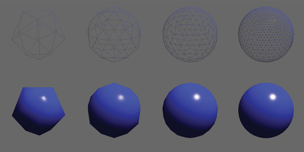
Per-fragment shading applied across increasing tessellation of a subdivision sphere. The specular highlight is apparent with lower tessellations.
lightPosID = shader.createUniform("light.position");
lightIntensityID = shader.createUniform("light.intensity");
17.13.3 A Normal Shader
Once you have a working shader program, such as the Blinn-Phong one presented here, it is easy to expand your ideas and develop new shaders. It may also be helpful to develop a set of very specific shaders for debugging. One such shader is the normal shader program. Normal shading is often helpful to understand whether the incoming geometry is organized correctly or whether the computations are correct. In this example, the vertex shader remains the same. Only the fragment shader changes:
#version 330 core
in vec4 normal;
layout (location=0) out vec4 fragmentColor;
void main(void)
{
// Notice the use of swizzling here to access
// only the xyz values to convert the normal vec4
// into a vec3 type !
vec3 intensity = normalize(normal.xyz) * 0.5 + 0.5;
fragmentColor = vec4(intensity, 1.0);
}
Whichever shaders you start building, be sure to comment them! The GLSL specification allows comments to be included in shader code, so leave yourself some details that can guide you later.
17.14 Meshes and Instancing
Once basic shaders are working, it’s interesting to start creating more complex scenes. Some 3D model files are simple to load and others require more effort. One simple 3D object file representation is the OBJ format. OBJ is a widely used format and several codes are available to load these types of files. The array of structs mechanism presented earlier works well for containing the OBJ data on the host. It can then easily be transferred into a VBO and vertex array objects.
Many 3D models are defined in their own local coordinate systems and need various transformations to align them with the OpenGL coordinate system. For instance, when the Stanford Dragon’s OBJ file is loaded into the OpenGL coordinate system, it appears lying on its side at the origin. Using GLM, we can create the model transformations to place objects within our scenes. For the dragon model, this means rotating −90 degrees about , and then translating up in . The effective model transform becomes
and the dragon is presented upright and above the ground plane, as shown in Figure 17.7. To do this we utilize several functions from GLM for generating local model transforms:

Images are described from left to right. The default local orientation of the dragon, lying on its side. After a -90 degree rotation about , the dragon is upright but still centered about the origin. Finally, after applying a translation of 1.0 in , the dragon is ready for instancing.
- glm::translate creates a translation matrix.
- glm::rotate creates a rotation matrix, specified in either degrees or radians about a specific axis.
- glm::scale creates a scale matrix.
We can apply these functions to create the model transforms and pass the model matrix to the shader using uniform variables. The Blinn-Phong vertex shader contains instructions that apply the local transform to the incoming vertex. The following code shows how the dragon model is rendered:
glUseProgram(BlinnPhongShaderID);
// Describe the Local Transform Matrix
glm::mat4 modelMatrix = glm::mat4(1.0); // Identity Matrix
modelMatrix = glm::translate(modelMatrix, glm::vec3 (0.0f, 1.0f, ↩
0.0f));
float rot = (-90.0f / 180.0f) * M_PI;
modelMatrix = glm:: rotate(modelMatrix, rot, glm::vec3(1, 0, 0));
// Set the Normal Matrix
glm::mat4 normalMatrix = glm::transpose (glm:: inverse (viewMatrix↩
* modelMatrix)) ;
// Pass the matrices to the GPU memory
glUniformMatrix4fv (nMatID, 1, GL_FALSE, glm::value_ptr(↩
normalMatrix));
glUniformMatrix4fv (pMatID, 1, GL_FALSE, glm:: value_ptr(projMatrix↩
));
glUniformMatrix4fv (vMatID, 1, GL_FALSE, glm::value_ptr(viewMatrix↩
));
glUniformMatrix4fv (mMatID, 1, GL_FALSE, glm::value_ptr(↩
modelMatrix));
// Set material for this object
glm::vec3 kd(0.2, 0.2, 1.0);
glm::vec3 ka = kd * 0.15f;
glm::vec3 ks(1.0, 1.0, 1.0);
float phongExp = 32.0;
glUniform3fv(kaID, 1, glm::value_ptr(ka));
glUniform3fv(kdID, 1, glm::value_ptr(kd));
glUniform3fv(ksID, 1, glm::value_ptr(ks));
glUniform1f(phongExpID, phongExp);
// Process the object and note that modelData.size() holds
// the number of vertices, not the number of triangles!
glBindVertexArray(VAO);
glDrawArrays(GL_TRIANGLES, 0, modelData.size());
glBindVertexArray(0);
glUseProgram(0);
17.14.1 Instancing Models
Instancing with OpenGL is implemented differently than instancing with the ray tracer. With the ray tracer, rays are inversely transformed into the local space of the object using the model transform matrix. With OpenGL, instancing is performed by loading a single copy of the object as a vertex array object (with associated vertex buffer objects), and then reusing the geometry as needed. Like the ray tracer, only a single object is loaded into memory, but many may be rendered.
Modern OpenGL nicely supports this style of instancing because vertex shaders can (and must) compute the necessary transformations to transform vertices into clip coordinates. By writing generalized shaders that embed these transformations, such as presented with the Blinn-Phong vertex shader, models can be rerendered with the same underlying local geometry. Different material types and transforms can be queried from higher-level class structures to populate the uniform variables passed from host to device each frame. Animations and interactive control are also easily created as the model transforms can change over time across the the display loop iteration. Figures 17.8 and 17.9 use the memory footprint of one dragon, yet render three different dragon models to the screen.

The results of running the Blinn-Phong shader program on the three dragons using uniform variables to specify material properties and transformations.

Setting the uniform variable ks = (0, 0, 0) in the Blinn-Phong shader program produces Lambertian shading.
17.15 Texture Objects
Textures are an effective means to manipulate visual effects with OpenGL shaders. They are used extensively with many hardware-based graphics algorithms and OpenGL supports them natively with Texture objects. Like the previous OpenGL concepts, texture objects must be allocated and initialized by copying data on the host to the GPU memory and setting OpenGL state. Texture coordinates are often integrated into the vertex buffer objects and passed as vertex attributes to shader programs. Fragment shaders typically perform the texture lookup function using interpolated texture coordinate passed from the vertex shaders.
Textures are rather simple to add to your code if you already have working shader and vertex array objects. The standard OpenGL techniques for creating objects on the hardware are used with textures. However, the source of the texture data must first be determined. Data can either be loaded from a file (e.g., PNG, JPG, EXR, or HDR image file formats) or generated procedurally on the host (and even on the GPU). After the data is loaded into host memory, the data is copied to GPU memory, and optionally, OpenGL state associated with textures can be set. OpenGL texture data is loaded as a linear buffer of memory containing the data used for textures. Texture lookups on the hardware can be 1D, 2D, or 3D queries. Regardless of the texture dimension query, the data is loaded onto the memory in the same way, using linearly allocated memory on the host. In the following example, the process of loading data from an image file (or generating it procedurally) is left to the reader, but variable names are provided that match what might be present if an image is loaded (e.g., imgData, imgWidth, imgHeight).
float *imgData = new float[imgHeight * imgWidth * 3];
...
GLuint texID;
glGenTextures(1, &texID);
glBindTexture(GL_TEXTURE_2D, texID);
glTexParameteri(GL_TEXTURE_2D, GL_TEXTURE_WRAP_S, GL_CLAMP);
glTexParameteri(GL_TEXTURE_2D, GL_TEXTURE_WRAP_T, GL_CLAMP);
glTexParameteri(GL_TEXTURE_2D, GL_TEXTURE_MAG_FILTER, GL_LINEAR);
glTexParameteri(GL_TEXTURE_2D, GL_TEXTURE_MIN_FILTER, GL_LINEAR);
glTexImage2D(GL_TEXTURE_2D, 0, GL_RGB, imgWidth, imgHeight, 0,
GL_RGB, GL_FLOAT, imgData);
glBindTexture(GL_TEXTURE_2D, 0);
delete [] imgData;
The example presented here highlights how to set up and use basic 2D OpenGL textures with shader programs. The process for creating OpenGL objects should be familiar by now. A handle (or ID) must be generated on the device to refer to the texture object (e.g., in this case, texID). The id is then bound to allow any subsequent texture state operations to affect the state of the texture. A fairly extensive set of OpenGL texture state and parameters exist that affect texture coordinate interpretation and texture lookup filtering. Various texture targets exist with graphics hardware. In this case, the texture target is specified as GL_TEXTURE_2D and will appear as the first argument in the texture-related functions. For OpenGL this particular texture target implies that texture coordinates will be specified in a device normalized manner (i.e., in the range of [0, 1]). Moreover, texture data must be allocated so that the width and height dimensions are powers of two (e.g., 512 × 512,1024 × 512, etc.). Texture parameters are set for the currently bound texture by calling glTexParameter. This signature for this function takes on a variety of forms depending on the types of data being set. In this case, texture coordinates will be clamped by the hardware to the explicit range [0,1]. The minifying and magnifying filters of OpenGL texture objects are set to use linear filtering (rather than nearest neighbor - GL_NEAREST) automatically when performing texture lookups. Chapter 11 provides substantial details on texturing, including details about the filtering that can occur with texture lookups. Graphics hardware can perform many of these operations automatically by setting the associated texture state.
Finally, the call to glTexImage2D performs the host to device copy for the texture. There are several arguments to this function, but the overall operation is to allocate space on the graphics card (e.g., imageWidth X imgHeight) of three floats (7th and 8th arguments: GL_RGB and GL_FLOAT) and copy the linear texture data to the hardware (e.g., imgData pointer). The remaining arguments deal with setting the mipmap level of detail (2nd argument), specifying the internal format (e.g., 3rd argument’s GL_RGB) and whether the texture has a border or not (6th argument). When learning OpenGL textures it is safe to keep these as the defaults listed here. However, the reader is advised to learn more about mipmaps and the potential internal formats of textures as more advanced graphics processing is required.
Texture object allocation and initialization happens with the code above. Additional modifications must be made to vertex buffers and vertex array objects to link in the correct texture coordinates with the geometric description. Following the previous examples, the storage for texture coordinates is a straightforward modification to the vertex data structure:
struct vertexData
{
glm::vec3 pos;
glm::vec3 normal;
glm::vec2 texCoord;
};
As a result, the vertex buffer object will increase in size and the interleaving of texture coordinates will require a change to the stride in the vertex attribute specification for the vertex array objects. Figure 17.10 illustrates the basic interleaving of data within the vertex buffer.

Data layout after adding the texture coordinate to the vertex buffer. Each block represents a GLfloat, which is 4 bytes. The position is encoded as a white block, the normals as purple, and the texture coordinates as orange.
glBindBuffer(GL_ARRAY_BUFFER, m_triangleVBO[0]);
glEnableVertexAttribArray(0);
glVertexAttribPointer(0, 3, GL_FLOAT, GL_FALSE, 8 * sizeof(GLfloat), 0);
glEnableVertexAttribArray(1);
glVertexAttribPointer(1, 3, GL_FLOAT, GL_FALSE, 8 * sizeof(GLfloat), (const GLvoid *)12);
glEnableVertexAttribArray(2);
glVertexAttribPointer(2, 2, GL_FLOAT, GL_FALSE, 8 * sizeof(GLfloat), (const GLvoid *)24);
glBindVertexArray(0);
With the code snippet above, the texture coordinates are placed at vertex attribute location 2. Note the change in size of the texture coordinate’s size (e.g., 2nd argument of glVertexAttribPointer is 2 for texture coordinates to coincide with the vec2 type in the structure). At this point, all initialization will have been completed for the texture object.
The texture object must be enabled (or bound) prior to rendering the vertex array object with your shaders. In general, graphics hardware allows the use of multiple texture objects when executing a shader program. In this way, shader programs can apply sophisticated texturing and visual effects. Thus, to bind a texture for use with a shader, it must be associated to one of potentially many texture units. Texture units represent the mechanism by which shaders can use multiple textures. In the sample below, only one texture is used so texture unit 0 will be made active and bound to our texture.
The function that activates a texture unit is glActiveTexture. Its only argument is the texture unit to make active. It is set to GL_TEXTURE0 below, but it could be GL_TEXTURE1 or GL_TEXTURE2, for instance, if multiple textures were needed in the shader. Once a texture unit is made active, a texture object can be bound to it using the glBindTexture call.
glUseProgram(shaderID);
glActiveTexture(GL_TEXTURE0);
glBindTexture(GL_TEXTURE_2D, texID);
glUniform1i(texUnitID, 0);
glBindVertexArray(VAO);
glDrawArrays(GL_TRIANGLES, 0, 3);
glBindVertexArray(0);
glBindTexture(GL_TEXTURE_2D, 0);
glUseProgram(0);
Most of the code above should be logical extensions to what you’ve developed thus far. Note the call to glUniform prior to rendering the vertex array object. In modern graphics hardware programming, shaders perform the work of texture lookups and blending, and therefore, must have data about which texture units hold the textures used in the shader. The active texture units are supplied to shaders using uniform variables. In this case, 0 is set to indicate that the texture lookups will come from texture unit 0. This will be expanded upon in the following section.
17.15.1 Texture Lookup in Shaders
Shader programs perform the lookup and any blending that may be required. The bulk of that computation typically goes into the fragment shader, but the vertex shader often stages the fragment computation by passing the texture coordinate out to the fragment shader. In this way, the texture coordinates will be interpolated and afford per-fragment lookup of texture data.
Simple changes are required to use texture data in shader programs. Using the Blinn-Phong vertex shader provided previously, only three changes are needed:
- The texture coordinates are a per-vertex attribute stored within the vertex array object. They are associated with vertex attribute index 2 (or location 2).
layout(location=2) in vec2 in_TexCoord; - The fragment shader will perform the texture lookup and will need an interpolated texture coordinate. This variable will be added as an output variable that gets passed to the fragment shader.
out vec2 tCoord; - Copy the the incoming vertex attribute to the output variable in the main function.
// Pass the texture coordinate to the fragment shader tCoord = in_TexCoord;
The fragment shader also requires simple changes. First, the incoming interpolated texture coordinates passed from the vertex shader must be declared. Also recall that a uniform variable should store the texture unit to which the texture is bound. This must be communicated to the shader as a sampler type. Samplers are a shading language type that allows the lookup of data from a single texture object. In this example, only one sampler is required, but in shaders in which multiple texture lookups are used, multiple sampler variables will be used. There are also multiple sampler types depending upon the type of texture object. In the example presented here, a GL_TEXTURE_2D type was used to create the texture state. The associated sampler within the fragment shader is of type sampler2D. The following two variable declarations must be added to the fragment shader:
in vec2 tCoord;
uniform sampler2D textureUnit;
The final modification goes into the main function of the fragment shader code. The texture is sampled using the GLSL texture lookup function and (in this case), replaces the diffuse coefficient of the geometry. The first argument to texture takes the sampler type which holds the texture unit to which the texture is bound. The second argument is the texture coordinate. The function returns a vec4 type. In the code snippet below, no alpha values are utilized in the final computation so the resulting texture lookup value is component-wise selected to only the RGB components. The diffuse coefficient from the texture lookup is set to a vec3 type that is used in the illumination equation.
vec3 kdTexel = texture(textureUnit, tCoord).rgb;
vec3 intensity = ka * Ia + kdTexel * light.intensity
* max(0.0, dot(n, l)) + ks * light.intensity
* pow(max(0.0, dot(n, h)), phongExp);
Figure 17.11 illustrates the results of using these shader modifications. The right-most image in the figure extends the example code by enabling texture tiling with the OpenGL state. Note that these changes are only done in host code and the shaders do not change. To enable this tiling, which allows for texture coordinates outside of the device normalized ranges, the texture parameters for GL_TEXTURE_WRAP_S and GL_TEXTURE_WRAP_T are changed from GL_CLAMP to GL_REPEAT. Additionally, the host code that sets the texture coordinates now ranges from [0, 5].
![Figure showing the left-most image shows the texture, a 1024 × 1024 pixel image. The middle image shows the scene with the texture applied using texture coordinates in the range of [0, 1] so that only one image is tiled onto the ground plane. The right-most image modifies the texture parameters so that GL_REPEAT is used for GL_TEXTURE_WRAP_S and GL_TEXTURE_WRAP_T and the texture coordinate range from [0, 5]. The result is a tiled texture repeat five times in both texture dimensions.](http://images-20200215.ebookreading.net/23/1/1/9781482229417/9781482229417__fundamentals-of-computer__9781482229417__image__fig17-11.png)
The left-most image shows the texture, a 1024 × 1024 pixel image. The middle image shows the scene with the texture applied using texture coordinates in the range of [0, 1] so that only one image is tiled onto the ground plane. The right-most image modifies the texture parameters so that GL_REPEAT is used for GL_TEXTURE_WRAP_S and GL_TEXTURE_WRAP_T and the texture coordinate range from [0, 5]. The result is a tiled texture repeat five times in both texture dimensions.
As a side note, another texture target that may be useful for various applications is the GL_TEXTURE_RECTANGLE. Texture rectangle are unique texture objects that are not constrained with the power-of-two width and height image requirements and use non-normalized texture coordinates. Furthermore, they do not allow repeated tiling. If texture rectangles are used, shaders must reference them using the special sampler type: sampler2DRect.
17.16 Object-Oriented Design for Graphics Hardware Programming
As your familiarity with OpenGL increases, it becomes wise to encapsulate most of what is described in this chapter into class structures that can contain the model specific data and afford rendering of a variety of objects within the scene. For instance, in Figure 17.12, a single sphere is instanced six times to create the three ellipsoids and three spheres. Each model uses the same underlying geometry yet has different material properties and model transforms. If you’ve followed through the book and implemented the ray tracer, as detailed in Chapter 4, then it is likely that your implementation is based on a solid object-oriented design. That design can be leveraged to make developing a graphics hardware program with OpenGL easier. A typical ray tracer software architecture will include several classes that map directly into graphics hardware as well as software rasterization applications. The abstract base classes in the ray tracer that represent surfaces, materials, lights, shaders, and cameras can be adapted to initialize the graphics hardware state, update that state, and if necessary render the class data to the framebuffer. The interfaces to these virtual functions will likely need to be adapted to your specific implementation, but a first pass that extends the surface class design might resemble the following:

On the left, a single tessellated sphere is instanced six times using different model transforms to create this scene using the per-fragment shader program. The image on the right is rendered using a basic Whitted ray tracer. Notice the effect that shadows have on the perception of the scene. Per-fragment shading allows the specular highlight to be similar in both rendering styles.
class surface
virtual bool initializeOpenGL()
virtual bool renderOpenGL(glm::mat4& Mp, glm::mat4& Mcam)
Passing the projection and view matrices to the render functions affords an indirection for how these matrices are managed. These matrices would come from the camera classes which may be manipulated by interpreting keyboard, mouse, or joystick input. The initialization functions (at least for the surface derivatives) would contain the vertex buffer object and vertex array object allocation and initialization code. Aside from initiating the draw arrays for any vertex array objects, the render function would also need to activate shader programs and pass in the necessary matrices into the shaders, as illustrated previously in the dragon model example. As you work to integrate the image-order and object-order (hardware and software) algorithms into the same underlying data framework, a few software design challenges will pop up, mostly related to data access and organization. However, this is a highly useful exercise to become adept at software engineering for graphics programming and eventually gain solid experience hybridizing your rendering algorithms.
17.17 Continued Learning
This chapter was designed to provide an introductory glimpse into graphics hardware programming, influenced by the OpenGL API. There are many directions that your continued learning could go. Many topics, such as framebuffer objects, render to texture, environment mapping, geometry shaders, compute shaders, and advanced illumination shaders were not covered. These areas represent the next stages in learning about graphics hardware, but even within the areas covered, there are many directions that one could go to develop stronger graphics hardware understanding. Graphics hardware programming will continue to evolve and change. Interested readers should expect these changes and look to the specification documents for OpenGL and the OpenGL Shading Language for many more details about what OpenGL is capable of doing and how the hardware relates to those computations.
Frequently Asked Questions
How do I debug shader programs?
On most platforms, debugging both vertex shaders and fragment shaders is not simple. However, more and more support is available through various drivers, operating system extensions, and IDEs to provide pertinent information to the developer. It still can be challenging, so use the shaders to visually debug your code. If nothing comes up on the screen, try rendering the normal vectors, the half vector, or anything that give you a sense for where the error might be (or not be). Figure 17.13 illustrates a normal shader in operation. If images do appear on your window, make sure they are what you expect (refer to Figure 17.14)!


Visual debugging is important! Can you figure out what is wrong from the image or where to start debugging? When the incorrect stride is applied to the vertex array object, rendering goes awry.
Notes
There are many good resources available to learn more about the technical details involved with programming graphics hardware. A good starting point might be the OpenGL and GLSL specification documents. They are available for free online at the opengl.org website. These documents will provide complete details for all the different and emerging versions of OpenGL.
Exercises
The sections of this chapter are roughly organized to step students through the process of creating a modern OpenGL application. Some extra effort will be required to understand the details relating to setting up windows and OpenGL contexts. However, it should be possible to following the sections for a set of weekly one hour labs:
- Lab 1: Basic code setup for OpenGL applications. This includes installing the necessary drivers and related software such as GLM and GLFW. Students can then write code to open a window and clear the color buffers.
- Lab 2: Creating a shader. Since a rudimentary shader is necessary to visualize the output in modern OpenGL, starting with efforts to create a very basic shader will go a long way. In this lab, or labs, students could build (or use provided) classes to load, compile, and link shaders into shader programs.
- Lab 3: Create a clip coordinate triangle and shade. Using the shader classes from the previous lab, students will add the passthrough shader and create simple geometry to render.
- Lab 4: Introduce GLM. Start using GLM to generate projection matrices and viewing matrices for viewing more generalized, yet simple, scenes.
- Lab 5: Use GLM for local transformations. Students can expand their working shader program to use local transforms, perhaps applying animations based on changing transforms.
- Lab 6: Shader development. Develop the Lambertian or Blinn-Phong shaders.
- Lab 7: Work with materials. Students can explore additional material properties and rendering styles with different shader programs.
- Lab 8: Load 3D models. Using code to load OBJ files, students can further explore the capabilities of their graphics hardware including the limits of hardware processing for real-time applications.
- Lab 9: Textures. Using PNG (or other formats), students can load images onto the hardware and practice a variety of texture-mapping strategies.
- Lab 10: Integration with rendering code. If scene files are used to describe scenes for the ray tracer (or rasterizer), students’ OpenGL code can be integrated into a complete rendering framework using common structures and classes to build a complete system.
This list is only a guide. In labs for my computer graphics course, students are provided material to get them started on the week’s idea. After they get the basic idea working, the lab is completed once they add their spin or a creative exploration of the idea to their code. As students get familiar with graphics hardware programming, they can explore additional areas of interest, such as textures, render to texture, or more advanced shaders and graphics algorithms.