
Chapter 19
Color
Erik Reinhard
Garrett Johnson
Photons are the carriers of optical information. They propagate through media taking on properties associated with waves. At surface boundaries they interact with matter, behaving more as particles. They can also be absorbed by the retina, where the information they carry is transcoded into electrical signals that are subsequently processed by the brain. It is only there that a sensation of color is generated.
As a consequence, the study of color in all its guises touches upon several different fields: physics for the propagation of light through space, chemistry for its interaction with matter, and neuroscience and psychology for aspects relating to perception and cognition of color (Reinhard et al., 2008).
In computer graphics, we traditionally take a simplified view of how light propagates through space. Photons travel along straight paths until they hit a surface boundary and are then reflected according to a reflection function of some sort. A single photon will carry a certain amount of energy, which is represented by its wavelength. Thus, a photon will have only one wavelength. The relationship between its wavelength λ and the amount of energy it carries (ΔE) is given by
where ΔE is measured in electron volts (eV).
In computer graphics, it is not very efficient to simulate single photons; instead large collections of them are simulated at the same time. If we take a very large number of photons, each carrying a possibly different amount of energy, then together they represent a spectrum. A spectrum can be thought of as a graph where the number of photons is plotted against wavelength. Because two photons of the same wavelength carry twice as much energy as a single photon of that wavelength, this graph can also be seen as a plot of energy against wavelength. An example of a spectrum is shown in Figure 19.1. The range of wavelengths to which humans are sensitive is roughly between 380 and 800 nanometers (nm).

A spectrum describes how much energy is available at each wavelength λ, here measured as relative radiant power. This specific spectrum represents average daylight.
When simulating light, it would therefore be possible to trace rays that each carry a spectrum. A renderer that accomplishes this is normally called a spectral renderer. From preceding chapters, it should be clear that we are not normally going through the expense of building spectral renderers. Instead, we replace spectra with representations that typically use red, green, and blue components. The reason that this is possible at all has to do with human vision and will be discussed later in this chapter.
Simulating light by tracing rays takes care of the physics of light, although it should be noted that several properties of light, including, for instance, polarization, diffraction, and interference, are not modeled in this manner.
At surface boundaries, we normally model what happens with light by means of a reflectance function. These functions can be measured directly by means of gonioreflectometers, leading to a large amount of tabled data, which can be more compactly represented by various different functions. Nonetheless, these reflectance functions are empirical in nature, i.e., they abstract away the chemistry that happens when a photon is absorbed and re-emitted by an electron. Thus, reflectance functions are useful for modeling in computer graphics, but do not offer an explanation as to why certain wavelengths of light are absorbed and others are reflected. We can therefore not use reflectance functions to explain why the light reflected off a banana has a spectral composition that appears to us as yellow. For that, we would have to study molecular orbital theory, a topic beyond the scope of this book.
Finally, when light reaches the retina, it is transcoded into electrical signals that are propagated to the brain. A large part of the brain is devoted to processing visual signals, part of which gives rise to the sensation of color. Thus, even if we know the spectrum of light that is reflected off a banana, we do not know yet why humans associate the term “yellow” with it. Moreover, as we will find out in the remainder of this chapter, our perception of color is vastly more complicated than it would seem at first glance. It changes with illumination, varies between observers, and varies within an observer over time.
In other words, the spectrum of light coming off a banana is perceived in the context of an environment. To predict how an observer perceives a “banana spectrum” requires knowledge of the environment that contains the banana as well as the observer’s environment. In many instances, these two environments are the same. However, when we are displaying a photograph of a banana on a monitor, then these two environments will be different. As human visual perception depends on the environment the observer is in, it may perceive the banana in the photograph differently from how an observer directly looking at the banana would perceive it. This has a significant impact on how we should deal with color and illustrates the complexities associated with color.
To emphasize the crucial role that human vision plays, we only have to look at the definition of color: “Color is the aspect of visual perception by which an observer may distinguish differences between two structure-free fields of view of the same size and shape, such as may be caused by differences in the spectral composition of the radiant energy concerned in the observation” (Wyszecki & Stiles, 2000). In essence, without a human observer there is no color.
Luckily, much of what we know about color can be quantified, so that we can carry out computations to correct for the idiosyncrasies of human vision and thereby display images that will appear to observers the way the designer of those images intended. This chapter contains the theory and mathematics required to do so.
19.1 Colorimetry
Colorimetry is the science of color measurement and description. Since color is ultimately a human response, color measurement should begin with human observation. The photodetectors in the human retina consist of rods and cones. The rods are highly sensitive and come into play in low-light conditions. Under normal lighting conditions, the cones are operational, mediating human vision. There are three cone types and together they are primarily responsible for color vision.
Although it may be possible to directly record the electrical output of cones while some visual stimulus is being presented, such a procedure would be invasive, while at the same time ignoring the sometimes substantial differences between observers. Moreover, much of the measurement of color was developed well before such direct recording techniques were available.
The alternative is to measure color by means of measuring the human response to patches of color. This leads to color matching experiments, which will be described later in this section. Carrying out these experiments have resulted in several standardized observers, which can be thought of as statistical approximations of actual human observers. First, however, we need to describe some of the assumptions underlying the possibility of color matching, which are summarized by Grassmann’s laws.
19.1.1 Grassmann’s Laws
Given that humans have three different cone types, the experimental laws of color matching can be summed up as the trichromatic generalization (Wyszecki & Stiles, 2000), which states that any color stimulus can be matched completely with an additive mixture of three appropriately modulated color sources. This feature of color is often used in practice, for instance by televisions and monitors which reproduce many different colors by adding a mixture of red, green, and blue light for each pixel. It is also the reason that renderers can be built using only three values to describe each color.
The trichromatic generalization allows us to make color matches between any given stimulus and an additive mixture of three other color stimuli. Hermann Grassmann was the first to describe the algebraic rules to which color matching adheres. They are known as Grassmann’s laws of additive color matching (Grassmann, 1853) and are the following:
- Symmetry law. If color stimulus A matches color stimulus B, then B matches A.
- Transitive law. If A matches B and B matches C, then A matches C.
- Proportionality law. If A matches B, then αA matches αB, where α is a positive scale factor.
- Additivity law. If A matches B, C matches D, and A + C matches B + D, then it follows that A + D matches B + C.
The additivity law forms the basis for color matching and colorimetry as a whole.
19.1.2 Cone Responses
Each cone type is sensitive to a range of wavelengths, spanning most of the full visible range. However, sensitivity to wavelengths is not evenly distributed, but contains a peak wavelength at which sensitivity is greatest. The location of this peak wavelength is different for each cone type. The three cone types are classified as S, M, and L cones, where the letters stand for short, medium, and long, indicating where in the visible spectrum the peak sensitivity is located.
The response of a given cone is then the magnitude of the electrical signal it outputs, as a function of the spectrum of wavelengths incident upon the cone. The cone response functions for each cone type as a function of wavelength λ are then given by L(λ), M(λ), and S(λ). They are plotted in Figure 19.2.

The actual response to a stimulus with a given spectral composition Ф(λ) is then given for each cone type by
These three integrated responses are known as tristimulus values.
19.1.3 Color Matching Experiments
Given that tristimulus values are created by integrating the product of two functions over the visible range, it is immediately clear that the human visual system does not act as a simple wavelength detector. Rather, our photo-receptors act as approximately linear integrators. As a result, it is possible to find two different spectral compositions, say Ф1(λ) and Ф2(λ), that after integration yield the same response (L, M, S). This phenomenon is known as metamerism, an example of which is shown in Figure 19.3.

Metamerism is the key feature of human vision that allows the construction of color reproduction devices, including the color figures in this book and anything reproduced on printers, televisions, and monitors.
Color matching experiments also rely on the principle of metamerism. Suppose we have three differently colored light sources, each with a dial to alter its intensity. We call these three light sources primaries. We should now be able to adjust the intensity of each in such a way that when mixed together additively, the resulting spectrum integrates to a tristimulus value that matches the perceived color of a fourth unknown light source. When we carry out such an experiment, we have essentially matched our primaries to an unknown color. The positions of our three dials are then a representation of the color of the fourth light source.
In such an experiment, we have used Grassmann’s laws to add the three spectra of our primaries. We have also used metamerism, because the combined spectrum of our three primaries is almost certainly different from the spectrum of the fourth light source. However, the tristimulus values computed from these two spectra will be identical, having produced a color match.
Note that we do not actually have to know the cone response functions to carry out such an experiment. As long as we use the same observer under the same conditions, we are able to match colors and record the positions of our dials for each color. However, it is quite inconvenient to have to carry out such experiments every time we want to measure colors. For this reason, we do want to know the spectral cone response functions and average those for a set of different observers to eliminate interobserver variability.
19.1.4 Standard Observers
If we perform a color matching experiment for a large range of colors, carried out by a set of different observers, it is possible to generate an average color matching dataset. If we specifically use monochromatic light sources against which to match our primaries, we can repeat this experiment for all visible wavelengths. The resulting tristimulus values are then called spectral tristimulus values, and can be plotted against wavelength λ, shown in Figure 19.4.

Spectral tristimulus values averaged over many observers. The primaries where monochromatic light sources with wavelengths of 435.8, 546.1, and 700 nm.
By using a well-defined set of primary light sources, the spectral tristimulus values lead to three color matching functions. The Commission Internationale d’Eclairage (CIE) has defined three such primaries to be monochromatic light sources of 435.8, 546.1, and 700 nm, respectively. With these three monochromatic light sources, all other visible wavelengths can be matched by adding different amounts of each. The amount of each required to match a given wavelength λ is encoded in color matching functions, given by , , and and plotted in Figure 19.4. Tristimulus values associated with these color matching functions are termed R, G, and B.
Given that we are adding light, and light cannot be negative, you may have noticed an anomaly in Figure 19.4: to create a match for some wavelengths, it is necessary to subtract light. Although there is no such thing as negative light, we can use Grassmann’s laws once more, and instead of subtracting light from the mixture of primaries, we can add the same amount of light to the color that is being matched.
The CIE , , and color matching functions allow us to determine if a spectral distribution Ф1 matches a second spectral distribution Ф2 by simply comparing the resulting tristimulus values obtained by integrating with these color matching functions:
Of course, a color match is only guaranteed if all three tristimulus values match.
The importance of these color matching functions lies in the fact that we are now able to communicate and describe colors compactly by means of tristimulus values. For a given spectral function, the CIE color matching functions provide a precise way in which to calculate tristimulus values. As long as everybody uses the same color matching functions, it should always be possible to generate a match.
If the same color matching functions are not available, then it is possible to transform one set of tristimulus values into a different set of tristimulus values appropriate for a corresponding set of primaries. The CIE has defined one such a transform for two specific reasons. First, in the 1930s numerical integrations were difficult to perform, and even more so for functions that can be both positive and negative. Second, the CIE had already developed the photopic luminance response function, CIE V(λ). It became desirable to have three integrating functions, of which V(λ) is one and all three being positive over the visible range.
To create a set of positive color matching functions, it is necessary to define imaginary primaries. In other words, to reproduce any color in the visible spectrum, we need light sources that cannot be physically realized. The color matching functions that were settled upon by the CIE are named , and and are shown in Figure 19.5. Note that is equal to the photopic luminance response function V(λ) and that each of these functions is indeed positive. They are known as the CIE 1931 standard observer.

The corresponding tristimulus values are termed X, Y, and Z, to avoid confusion with R, G, and B tristimulus values that are normally associated with realizable primaries. The conversion from (R, G, B) tristimulus values to (X, Y, Z) tristimulus values is defined by a simple 3×3 transform:
To calculate tristimulus values, we typically directly integrate the standard observer color matching functions with the spectrum of interest Ф(λ), rather than go through the CIE , , and color matching functions first, followed by the above transformation. It allows us to calculate consistent color measurements and also determine when two colors match each other.
19.1.5 Chromaticity Coordinates
Every color can be represented by a set of three tristimulus values (X, Y, Z). We could define an orthogonal coordinate system with X, Y, and Z axes and plot each color in the resulting 3D space. This is called a color space. The spatial extent of the volume in which colors lie is then called the color gamut.
Visualizing colors in a 3D color space is fairly difficult. Moreover, the Y-value of any color corresponds to its luminance, by virtue of the fact that equals V(λ). We could therefore project tristimulus values to a 2D space which approximates chromatic information, i.e., information which is independent of luminance. This projection is called a chromaticity diagram and is obtained by normalization while at the same time removing luminance information:
Given that x + y + z equals 1, the z-value is redundant, allowing us to plot the x and y chromaticities against each other in a chromaticity diagram. Although x and y by themselves are not sufficient to fully describe a color, we can use these two chromaticity coordinates and one of the three tristimulus values, traditionally Y, to recover the other two tristimulus values:
By plotting all monochromatic (spectral) colors in a chromaticity diagram, we obtain a horseshoe-shaped curve. The points on this curve are called spectrum loci. All other colors will generate points lying inside this curve. The spectrum locus for the 1931 standard observer is shown in Figure 19.6. The purple line between either end of the horseshoe does not represent a monochromatic color, but rather a combination of short and long wavelength stimuli.

A (non-monochromatic) primary can be integrated over all visible wavelengths, leading to (X, Y, Z) tristimulus values, and subsequently to an (x, y) chromaticity coordinate, i.e., a point on a chromaticity diagram. Repeating this for two or more primaries yields a set of points on a chromaticity diagram that can be connected by straight lines. The volume spanned in this manner represents the range of colors that can be reproduced by the additive mixture of these primaries. Examples of three-primary systems are shown in Figure 19.7.
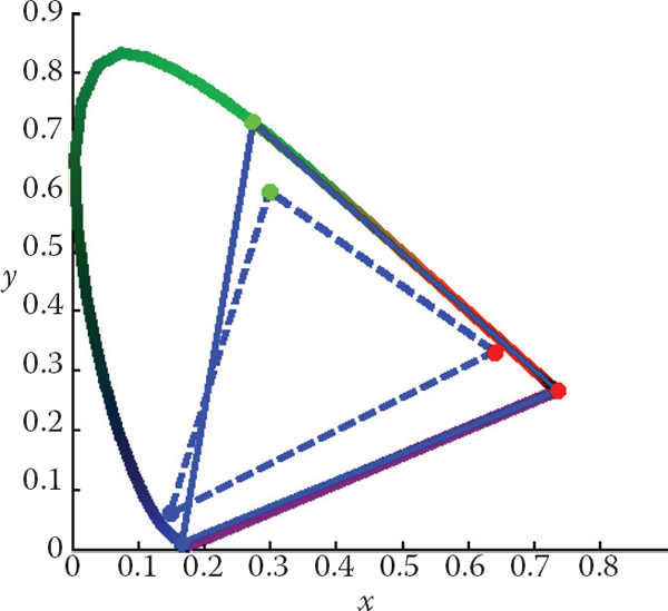
The chromaticity boundaries of the CIE RGB primaries at 435.8, 546.1, and 700 nm (solid) and a typical HDTV (dashed).
Chromaticity diagrams provide insight into additive color mixtures. However, they should be used with care. First, the interior of the horseshoe should not be colored, as any color reproduction system will have its own primaries and can only reproduce some parts of the chromaticity diagram. Second, as the CIE color matching functions do not represent human cone sensitivities, the distance between any two points on a chromaticity diagram is not a good indicator for how differently these colors will be perceived.
A more uniform chromaticity diagram was developed to at least in part address the second of these problems. The CIE u'v' chromaticity diagram provides a perceptually more uniform spacing and is therefore generally preferred over (x, y) chromaticity diagrams. It is computed from (X, Y, Z) tristimulus values by applying a different normalization,
and can alternatively be computed directly from (x, y) chromaticity coordinates:
A CIE u'v' chromaticity diagram is shown in Figure 19.8.

19.2 Color Spaces
As explained above, each color can be represented by three numbers, for instance defined by (X, Y, Z) tristimulus values. However, its primaries are imaginary, meaning that it is not possible to construct a device that has three light sources (all positive) that can reproduce all colors in the visible spectrum.
For the same reason, image encoding and computations on images may not be practical. There is, for instance, a large number of possible XYZ values that do not correspond to any physical color. This would lead to inefficient use of available bits for storage and to a higher requirement for bit-depth to preserve visual integrity after image processing. Although it may be possible to build a capture device that has primaries that are close to the CIE XYZ color matching functions, the cost of hardware and image processing make this an unattractive option. It is not possible to build a display that corresponds to CIE XYZ. For these reasons, it is necessary to design other color spaces: physical realizability, efficient encoding, perceptual uniformity, and intuitive color specification.
The CIE XYZ color space is still actively used, mostly for the conversion between other color spaces. It can be seen as a device-independent color space.
Other color spaces can then be defined in terms of their relationship to CIE XYZ, which is often specified by a specific transform. For instance, linear and additive trichromatic display devices can be transformed to and from CIE XYZ by means of a simple 3 × 3 matrix. Some nonlinear additional transform may also be specified, for instance to minimize perceptual errors when data is stored with a limited bit-depth, or to enable display directly on devices that have a nonlinear relationship between input signal and the amount of light emitted.
19.2.1 Constructing a Matrix Transform
For a display device with three primaries, say red, green, and blue, we can measure the spectral composition of the emitted light by sending the color vectors (1,0, 0), (0,1, 0), and (0, 0,1). These vectors represent the three cases namely where one of the primaries is full on, and the other two are off. From the measured spectral output, we can then compute the corresponding chromaticity coordinates (xR,yR), (xG,yG), and (xB,yB).
The white point of a display is defined as the spectrum emitted when the color vector (1,1,1) is sent to the display. Its corresponding chromaticity coordinate is (xW, yW). The three primaries and the white point characterize the display and are each required to construct a transformation matrix between the display’s color space and CIE XYZ.
These four chromaticity coordinates can be extended to chromaticity triplets reconstructing the z-coordinate from z = 1−x−y, leading to triplets (xR, yR, zR), (xG, yG, zG), (xB, yB, zB), and (xW, yW, zW). If we know the maximum luminance of the white point, we can compute its corresponding tristimulus value (XW, YW, ZW) and then solve the following set of equations for the luminance ratio scalars SR, SG, and SB:
The conversion between RGB and XYZ is then given by
The luminance of any given color can be computed by evaluating the middle row of a matrix constructed in this manner:
To convert between XYZ and RGB of a given device, the above matrix can simply be inverted.
If an image is represented in an RGB color space for which the primaries and white point are unknown, then the next best thing is to assume that the image was encoded in a standard RGB color space. A reasonable choice is then to assume that the image was specified according to ITU-R BT.709, which is the specification used for encoding and broadcasting of HDTV. Its primaries and white point are specified in Table 19.1. Note that the same primaries and white point are used to define the well-known sRGB color space. The transformation between this RGB color space and CIE XYZ is and vice versa given by
The (x, y) chromaticity coordinates for the primaries and white point specified by ITU-R BT.709. The sRGB standard also uses these primaries and white point.
R |
G |
B |
White |
|
|---|---|---|---|---|
x |
0.6400 |
0.3000 |
0.1500 |
0.3127 |
y |
0.3300 |
0.6000 |
0.0600 |
0.3290 |
By substituting the maximum RGB values of the device, we can compute the white point. For ITU-R BT.709, the maximum values are (RW, GW, BW) = (100,100,100), leading to a white point of (XW, YW, ZW) = (95.05,100.00, 108.90).
In addition to a linear transformation, the sRGB color space is characterized by a subsequent nonlinear transform. The nonlinear encoding is given by
This nonlinear encoding helps minimize perceptual errors due to quantization errors in digital applications.
19.2.2 Device-Dependent RGB Spaces
As each device typically has its own set of primaries and white point, we call the associated RGB color spaces device-dependent. It should be noted that even if all these devices operate in an RGB space, they may have very different primaries and white points. If we therefore have an image specified in some RGB space, it may appear very different to us, depending upon which device we display it.
This is clearly an undesirable situation, resulting from a lack of color management. However, if the image is specified in a known RGB color space, it can first be converted to XYZ, which is device independent, and then subsequently it can be converted to the RGB space of the device on which it will be displayed.
There are several other RGB color spaces that are well defined. They each consist of a linear matrix transform followed by a nonlinear transform, akin to the aforementioned sRGB color space. The nonlinear transform can be parameterized as follows:
The parameters s, f, t and γ, together with primaries and white point, specify a class of RGB color spaces that are used in various industries. Several common transformations are listed in Table 19.2.
Transformations for standard RGB color spaces (after (Pascale, 2003)).
Color space |
XYZ to RGB matrix |
RGB to XYZ matrix |
Nonlinear transform |
|---|---|---|---|
sRGB3 |
|||
Adobe RGB (1998) |
|
||
HDTV (HD-CIF) |
|||
NTSC (1953)/ITU-R BT.601-4 |
|||
PAL/SECAM |
|||
SMPTE-C |
|||
SMPTE-240M |
|||
Wide Gamut |
19.2.3 LMS Cone Space
The aforementioned cone signals can be expressed in terms of the CIE XYZ color space. The matrix transform to compute LMS signals from XYZ and vice versa are given by
This transform is known as the Hunt-Pointer-Estevez transform (Hunt, 2004) and is used in chromatic adaptation transforms as well as in color appearance modeling.
19.2.4 CIE 1976 L*a*b*
Color opponent spaces are characterized by a channel representing an achromatic channel (luminance), as well as two channels encoding color opponency. These are frequently red-green and yellow-blue channels. These color opponent channels thus encode two chromaticities along one axis, which can have both positive and negative values. For instance, a red-green channel encodes red for positive values and green for negative values. The value zero encodes a special case: neutral which is neither red or green. The yellow-blue channel works in much the same way.
As at least two colors are encoded on each of the two chromatic axes, it is not possible to encode a mixture of red and green. Neither is it possible to encode yellow and blue simultaneously. While this may seem a disadvantage, it is known that the human visual system computes similar attributes early in the visual pathway. As a result, humans are not able to perceive colors that are simultaneously red and green, or yellow and blue. We do not see anything resembling reddish-green, or yellowish-blue. We are, however, able to perceive mixtures of colors such as yellowish-red (orange) or greenish-blue, as these are encoded across the chromatic channels.
The most relevant color opponent system for computer graphics is the CIE 1976 L*a*b* color model. It is a perceptually more or less uniform color space, useful, among other things, for the computation of color differences. It is also known as CIELAB.
The input to CIELAB are the stimulus (X, Y, Z) tristimulus values as well as the tristimulus values of a diffuse white reflecting surface that is lit by a known illuminant, (Xn, Yn, Zn). CIELAB therefore goes beyond being an ordinary color space, as it takes into account a patch of color in the context of a known illumination. It can thus be seen as a rudimentary color appearance space.
The three channels defined in CIELAB are L*, a*, and b*. The L* channel encodes the lightness of the color, i.e., the perceived reflectance of a patch with tristimulus value (X, Y, Z). The a* and b* are chromatic opponent channels. The transform between XYZ and CIELAB is given by
The function f is defined as
As can be seen from this formulation, the chromatic channels do depend on the luminance Y. Although this is perceptually accurate, it means that we cannot plot the values of a* and b* in a chromaticity diagram. The lightness L* is normalized between 0 and 100 for black and white. Although the a* and b* channels are not explicitly constrained, they are typically in the range [−128,128].
As CIELAB is approximately perceptually linear, it is possible to take two colors, convert them to CIELAB, and then estimate the perceived color difference by computing the Euclidean distance between them. This leads to the following color difference formula:
The letter E stands for difference in sensation (in German, Empfindung) (Judd, 1932).
Finally, the inverse transform between CIELAB and XYZ is given by
19.3 Chromatic Adaptation
The CIELAB color space just described takes as input both a tristimulus value of the stimulus and the tristimulus value of light reflected off a white diffuse patch. As such, it forms the beginnings of a system in which the viewing environment is taken into account.
The environment in which we observe objects and images has a large influence on how we perceive those objects. The range of viewing environments that we encounter in daily life is very large, from sunlight to starlight and from candlelight to fluorescent light. The lighting conditions not only constitute a very large range in the amount of light that is present, but also vary greatly in the color of the emitted light.
The human visual system accommodates these changes in the environment through a process called adaptation. Three different types of adaptation can be distinguished, namely light adaptation, dark adaptation, and chromatic adaptation. Light adaptation refers to the changes that occur when we move from a very dark to a very light environment. When this happens, at first we are dazzled by the light, but soon we adapt to the new situation and begin to distinguish objects in our environment. Dark adaptation refers to the opposite—when we go from a light environment to a dark environment. At first, we see very little, but after a given amount of time, details will start to emerge. The time needed to adapt to the dark is generally much longer than for light adaptation.
Chromatic adaptation refers to our ability to adapt, and largely ignore, variations in the color of the illumination. Chromatic adaptation is, in essence, the biological equivalent of the white balancing operation that is available on most modern cameras. The human visual system effectively normalizes the viewing conditions to present a visual experience that is fairly consistent. Thus, we exhibit a certain amount of color constancy: object reflectances appear relatively constant despite variations in illumination.
Although we are able to largely ignore changes in viewing environment, we are not able to do so completely. For instance, colors appear much more colorful on a sunny day than they do on a cloudy day. Although the appearances have changed, we do not assume that object reflectances themselves have actually changed their physical properties. We thus understand that the lighting conditions have influenced the overall color appearance.
Nonetheless, color constancy does apply to chromatic content. Chromatic adaptation allows white objects to appear white for a large number of lighting conditions, as shown in Figure 19.9.

A series of light sources plotted in the CIE u′v′ chromaticity diagram. A white piece of paper illuminated by any of these light sources maintains a white color appearance.
Computational models of chromatic adaptation tend to focus on the gain control mechanism in the cones. One of the simplest models assumes that each cone adapts independently to the energy that it absorbs. This means that different cone types adapt differently dependent on the spectrum of the light being absorbed. Such adaptation can then be modeled as an adaptive and independent rescaling of the cone signals:
where (La, Ma, Sa) are the chromatically adapted cone signals, and α, β, and γ are the independent gain controls which are determined by the viewing environment. This type of independent adaptation is also known as von-Kries adaptation. An example is shown in Figure 19.10.

An example of von Kries–style independent photoreceptor gain control. The relative cone responses (solid line) and the relative adapted cone responses to CIE illuminant A (dashed) are shown. The separate patch of color represents CIE illuminant A rendered into the sRGB color space.
The adapting illumination can be measured off a white surface in the scene. In the ideal case, this would be a Lambertian surface. In a digital image, the adapting illumination can also be approximated as the maximum tristimulus values of the scene. The light measured or computed in this manner is the adapting white, given by (Lw, Mw, Sw). Von Kries adaptation is then simply a scaling by the reciprocal of the adapting white, carried out in cone response space:
In many cases, we are interested in what stimulus should be generated under one illumination to match a given color under a different illumination. For example, if we have a colored patch illuminated by daylight, we may ask ourselves what tristimulus values should be generated to create a matching color patch that will be illuminated by incandescent light.
We are thus interested in computing corresponding colors, which can be achieved by cascading two chromatic adaptation calculations. In essence, the previously mentioned von Kries transform divides out the adapting illuminant—in our example, the daylight illumination. If we subsequently multiply in the incandescent illuminant, we have computed a corresponding color. If the two illuminants are given by (Lw,1, Mw,1, Sw,1) and (Lw,2, Mw,2, Sw,2), the corresponding color (Lc, Mc, Sc) is given by
There are several more complicated and, therefore, more accurate chromatic adaptation transform in existence (Reinhard et al., 2008). However, the simple von Kries model remains remarkably effective in modeling chromatic adaptation and can thus be used to achieve white balancing in digital images.
The importance of chromatic adaptation in the context of rendering, is that we have moved one step closer to taking into account the viewing environment of the observer, without having to correct for it by adjusting the scene and rerendering our imagery. Instead, we can model and render our scenes, and then, as an image postprocess, correct for the illumination of the viewing environment. To ensure that white balancing does not introduce artifacts, however, it is important to ensure that the image is rendered to a floating-point format. If rendered to traditional 8-bit image formats, the chromatic adaptation transform may amplify quantization errors.
19.4 Color Appearance
While colorimetry allows us to accurately specify and communicate color in a device-independent manner, and chromatic adaptation allows us to predict color matches across changes in illumination, these tools are still insufficient to describe what colors actually look like.
To predict the actual perception of an object, we need to know more information about the environment and take that information into account. The human visual system is constantly adapting to its environment, which means that the perception of color will be strongly influenced by such changes. Color appearance models take into account measurements of the stimulus itself, as well as the viewing environment. This means that the resulting description of color is independent of viewing condition.
The importance of color appearance modeling can be seen in the following example. Consider an image being displayed on an LCD screen. When making a print of the same image and viewing it in a different context, more often than not the image will look markedly different. Color appearance models can be used to predict the changes required to generate an accurate cross-media color reproduction (Fairchild, 2005).
Although color appearance modeling offers important tools for color reproduction, actual implementations tend to be relatively complicated and cumbersome in practical use. It can be anticipated that this situation may change over time. However, until then, we leave their description to more specialized textbooks (Fairchild, 2005).
Notes
Of all the books on color theory, Reinhard et al.’s work (Reinhard et al., 2008) is most directly geared toward engineering disciplines, including computer graphics, computer vision, and image processing. Other general introductions to color theory are given by Berns (Berns, 2000) and Stone (Stone, 2003). Wyszecki and Stiles have produced a comprehensive volume of data and formulae, forming an indispensable reference work (Wyszecki & Stiles, 2000). For color reproduction, we recommend Hunt’s book (Hunt, 2004). Color appearance models are comprehensively described in Fairchild’s book (Fairchild, 2005). For color issues related to video and HDTV Poynton’s book is essential (Poynton, 2003).