CHAPTER 6
Forward and Futures Contracts
INTRODUCTION
In order to understand forward and futures contracts, let us commence our discussion with an illustration of a spot transaction. Assume that we are standing on 15 May 20XX and that we wish to buy 100 shares of ABC. We will go to an exchange like the NYSE and place a buy order for 100 shares of ABC stock. The order will be matched with a sell order placed by another party, assuming that a suitable counterparty is available, and a trade will be executed for 100 shares. Such a transaction is termed as a cash or a spot transaction. This is because as soon as a deal is struck between the buyer and the seller, the buyer has to immediately make arrangements for the cash to be transferred to the seller, while the seller has to ensure that the right to the asset in question, in this case shares of ABC, is immediately transferred to the buyer.
Now consider a slightly different situation. Assume that on 15 May 20XX we wish to enter into a contract to acquire 100 shares of ABC on 15 August 20XX, and that a counterparty exists who is willing to sell the shares on that day. If so, we can enter into a contract that entails the payment of cash on 15 August against delivery of shares on the same day. The difference as compared to the earlier transaction is that no money need be paid by the buyer at the time of negotiating the contract, and neither does the seller need to transfer rights to the underlying asset on that day. The actual exchange of cash for the asset will take place on the transaction date specified in the contract, which in this case is 15 August. Such a contract is termed as a forward contract, for it entails the negotiation of terms and conditions in advance for a trade that is scheduled to take place on a future date.
In a forward contract, at the time of negotiating the deal the two parties have to agree on the terms at which they will transact on the future date. The following need to be clearly spelled out: (1) the underlying asset, in this case shares of ABC; and (2) the contract size, in this case 100 shares. The delivery date and the transaction venue should also be agreed upon. In our illustration the delivery date is 15 August, and we will assume that the venue for the exchange is New York City. Finally, the price at which the deal will be consummated on 15 August should also be fixed at the time of negotiating on 15 May. Let us assume that the price that is agreed upon is $80 per share.
A forward contract is termed as a commitment contract, for it represents an unconditional commitment to buy the underlying asset on the part of the buyer and an equivalent commitment to sell on the part of the seller. If the buyer were to renege by not paying the contractual amount on 15 August, it would be tantamount to default. Similarly, if the seller were to refuse to part with the shares on that day, it would be construed as default.
In every forward contract there will be a party who agrees to buy the underlying asset and a party who agrees to sell the underlying asset. The first party is termed as the buyer or the long, while the counterparty is designated as the seller or the short.
A forward contract is a customized or a private or an OTC contract. The term OTC, which stands for Over-the-Counter, connotes that such trades are not executed on an organized exchange. That is, a forward contract such as the one that we have described will not take place on an exchange like the NYSE. Such contracts are negotiated privately between a potential buyer and a potential seller. They are referred to as customized agreements because the two parties are at liberty to specify any terms and conditions that they can mutually agree upon. Let us consider the forward contract on shares of ABC. We have specified the underlying asset as shares of ABC. In practice the asset could be shares of any other stock, or even a nonfinancial product such as gold or wheat. The contract size has been assumed to be 100 shares. This too was arbitrarily fixed. While two parties, say Alfred and Colin, may agree to transact in 100 shares of ABC stock, two others, say Molly and Patsy, may agree on 175 shares of ABC stock. The transaction date has been set as 15 August 20XX. There is no sanctity about this date, and the potential buyer and seller are at liberty to arrive at any transaction date by consensus. Finally, we have assumed that the location for the trade is New York City. This was chosen arbitrarily as well, and the two parties may agree on any location of their choice. Thus, in the case of a forward contract all features such as the underlying asset, the quantum of the underlying asset, the date of delivery, and the place of delivery are arrived at by bilateral discussions between the potential buyer and the seller. Needless to say, the transaction price that is fixed at the outset is also determined by a process of negotiation between the two parties.
In these contracts there is obviously a major risk of default. Let us analyze the rationale. Assume that Alfred agrees to acquire 500 shares of ABC from Bob on 15 August 20XX. The agreement is entered into on 15 May 20XX and the price is fixed at $80 per share. On 15 August there are two possibilities. The market price for a cash or spot transaction may be less than 80 or more than 80. If the price were to be less than $80 per share, Alfred would be unwilling to pay $80 per share if he can get away with it. Thus, if the spot price on the scheduled transaction date were to be less than the forward price, the long will have an incentive to renege. But what if the spot price on 15 August were to be more than $80 per share? If so, the seller will be unwilling to sell the asset for the contracted price. In other words, if the spot price on the scheduled date were to be greater than the forward price, the short has an incentive to default. Thus, default risk is an integral part of such contracts. It is for this reason that forward contracts are primarily between institutional parties such as commercial banks, investment banks, large corporations, and insurance companies. Such parties have the resources and skills to assess the credibility of a potential counterparty. Forward contracts are extremely popular in the foreign exchange market where importers and exporters routinely enter into such transactions with commercial banks.
Now let us turn our attention to another product known as a futures contract. It too is a commitment contract that is written on an underlying asset; however, it is offered by an organized futures exchange and is not an OTC product. The most famous futures exchange in the world is the CME Group based in Chicago, and we will illustrate such contracts with an example from this exchange.
Consider the corn futures contract on this exchange. Each contract is for 5,000 bushels of the commodity. Quite obviously the contract can be used only by traders who wish to transact in multiples of 5,000 bushels. The exchange specifies three deliverable grades: #1 Yellow; #2 Yellow; and #3 Yellow. Thus, transactions are feasible in only the specified grades. The contract months available are March, May, July, September, and December. Thus, if two traders wish to transact on 15 August 20XX, as we assumed in our earlier illustration, they cannot use these contracts. The last delivery date as per the specifications of the exchange is the second business day following the last trading day of the delivery month, and the last trading date is the business day prior to the 15th calendar day of the contract month. Consider the futures contracts expiring in July 20XX. The last trading day is Wednesday 14 July, and the last delivery date is Friday the 16th of July. Hence if two parties desire to effect delivery on the 25th of July 20XX, then such contracts are unsuitable.
As can be deduced from this example, futures contracts are standardized contracts. That is, unlike forward contracts where the terms and conditions are set based on bilateral negotiations, in futures contracts there is a third party that specifies the permitted terms and conditions. This third party is the futures exchange. Such an exchange may be a stand-alone entity such as the CME Group, or it may be a division of a stock exchange. The exchange will specify the following features in the case of a futures contract.
The contract size: In our illustration it is 5,000 bushels. Thus, traders can take positions only in multiples of this amount.
The allowable grades: In our illustration the exchange has specified three allowable grades for corn. Thus, transactions in any other variety of the product are ruled out.
The allowable locations: In some cases, the exchange will specify more than one location where the underlying asset can be delivered. Thus, delivery has to be made at only the locations specified in the contract.
The delivery date/window: The exchange may specify a specific date on which delivery can be made. In practice it is more common to specify a delivery window. Thus, delivery can be made only between the start and end dates specified by the exchange. In the case of corn futures, the first delivery date is the first business of the expiration month, which is 1 July 20XX for the July contract. The last delivery date is the second business day following the last trading day of the delivery month, which is 16 July 20XX.
What are the consequences of such standardization? First, it reduces transactions costs. The cost of negotiating a customized agreement where each clause has to be drafted after painstaking negotiations will be much higher. Second, the trading volumes and the liquidity of futures contracts is much higher since only a few types of contracts are eligible for trading for each underlying product.
The futures exchange will have an associated entity known as a clearinghouse. The clearinghouse will position itself as the counterparty for each of the two original parties to the trade. That is, once a trade is consummated between a buyer and a seller, the clearinghouse will intervene and position itself as the effective seller from the standpoint of the buyer, and as the effective buyer from the perspective of the seller. Thus, the link between the two original parties is severed by the clearinghouse. It must be noted that neither of the parties to the trade actually trades with the clearinghouse. The clearinghouse intervenes and positions itself as a central counterparty only after the trade is consummated. The clearinghouse essentially reduces the risk of default for the two parties to the trade. Once the clearinghouse enters the picture, each of the two parties has to only worry about the strength and integrity of the clearinghouse and not about the original counterparty. The clearinghouse also makes it easier to offset the transaction.
What is offsetting? The term offsetting, also referred to as the assumption of a counterposition, entails the taking of a short position by a trader who has previously gone long, or by the taking of a long position by an investor who has earlier gone short.
A forward contract is a customized contract between two parties. Thus, a party who is seeking to offset or abrogate an existing position has to approach the original counterparty and have the agreement canceled. For instance, assume that Sterling Infotech, a software company based in Bangalore, has entered into a forward contract with HSBC to sell 250,000 USD to the bank after three months at a rate of INR 75.0000 per dollar. But one month after entering into the contract Sterling finds that its US customer has gone bankrupt and the receivable in dollars will not materialize. Sterling then has to approach the bank and have the original agreement canceled.
The cancellation of a futures position, however, is a lot easier and does not require the canceling party to approach the party with which it traded initially. Assume that Ray, a trader in Kansas City, has gone long in 100 futures contracts on wheat, with a counterparty in Des Moines. In this case, the order would have been routed through an exchange like the CME Group. The bilateral auction process on such exchanges is such that the trading parties would not even be aware of their counterparty's identity. Assume that two weeks after the transaction, Ray wishes to offset his long position. All he has to do is to contact a broker and have a sell order placed for 100 futures contracts on wheat. This time, the counterparty with whom the trade is effected need not be the party in Des Moines with whom he had originally traded, and in practice could be anybody who wishes to go long at that instant. Let us assume that this time the party who trades with Ray is based in Bloomington. As far as the records of the clearinghouse are concerned, they will reflect the fact that Ray had initially gone long in 100 contracts on wheat, and that he has subsequently gone short in 100 contracts on the same asset. His net position after the second transaction will be nil, and consequently he has no further obligations from the standpoint of giving or taking delivery.
To offset a futures position, the offsetting order must be on the same underlying asset, and for a contract expiring in the same month. For instance, if Ray had initially gone long in wheat futures expiring in September, he should subsequently go short in futures on the same underlying commodity, which are scheduled to expire in the same expiration month, September. The price at which the original trade was consummated need not be the same as the price at which the offsetting order is placed. Thus, Ray may exit the market with either a profit or a loss. If we assume that he went long at $4.25 per bushel and that he subsequently offset at $4.95 per bushel, his profit/loss will be:
There are two reasons why futures contracts are easy to offset. First, contracts on the underlying product, in this case wheat, have to be designed as per the specifications of the exchange. In this case each contract has to be for 5,000 bushels, with the same allowable grade/grades, and with the same delivery schedule. Thus, the nature of Ray's initial contract with the party in Des Moines will be identical to that of the subsequent offsetting contract with the party in Bloomington. Second, once Ray's initial trade is consummated, the link between him and the counterparty in Des Moines is broken because the clearinghouse has subsequently positioned itself as the effective counterparty to the trade. On the other hand, forward contracts are typically for nonstandard sizes, products, and delivery dates. Consequently, they can be offset only with the approval of the original counterparty. In addition, the identity of this party remains critical for there is no intervening entity, such as a clearinghouse.
The clearinghouse provides both original counterparties with a guarantee against the specter of default. The issue is, how can such a guarantee be implemented in practice? In order to ensure that neither party has to worry about the possibility of default on the part of the other, the clearinghouse will estimate the potential loss for each party and collect it in advance. This deposit is referred to as a margin and is a performance guarantee or good-faith deposit. The rationale is that if a party were to default after providing such a margin, then the funds held by the clearinghouse will be adequate to take care of the interests of the counterparty. In a futures contract, both parties have a commitment to perform, and the possibility of default exists for both a priori. Consequently, both the long and the short are required to deposit margins immediately after the trade. The margin that is deposited at the outset is referred to as the initial margin.
If a margin is collected at the very outset, it need not imply that both parties will be protected against default until the very end. What would happen, for instance, if a major price move led to a substantial erosion of margin for one of the two parties, thereby putting the counterparty at risk once again? Thus there is a need to periodically assess the level of margin posted by a party and make adjustments for prior profits and losses. To understand how the mechanism works in practice, we need to introduce the concepts of marking to market, and maintenance/variation margins.
The loss or gain accruing to a party to a futures trade arises over a period of time. As a result, there is a need to periodically compute the gain/loss for a party and adjust the margin position accordingly. In practice, futures exchanges do this at the close of trading every day, a procedure called marking to market. While marking to market, the clearinghouse will compute the profit for a party from the time the contract was previously marked to market. Gains will be credited to the margin account and losses will be debited. Futures contracts are marked to market for the first time on the day that the position is entered into. Subsequently they are marked to market on every business day until the contract expires, or is offset by the party, if that were to happen earlier. The principle for computing the profit/loss is the following.
Assume that traders have gone long in a contract at a price of F0. Assume that the price at the end of the day is F1. If they were to offset at the end of the day, it would be tantamount to agreeing to sell the underlying asset, which they had earlier agreed to buy at F0, at a price of F1. If F1 > F0, they will obviously have a profit; if not, they will have a loss. While marking to market, the clearinghouse will compute the profit/loss assuming that the party is offsetting and will credit/debit the margin account accordingly. Because the party has not actually expressed a desire to offset, however, the clearinghouse will reopen the position at the price at which the offset was assumed to have taken place.
Thus, rising futures prices lead to profits for the long, while declining prices lead to losses. It can be logically deduced that the situation for the shorts is exactly the opposite; rising futures prices will lead to losses, while falling prices will imply profits. All futures contracts are marked to market every day. The price used for this purpose is referred to as the settlement price. This may be the closing price for the day, although many exchanges use a volume-weighted average of prices observed during the last phase of trading for the day. If a contract is inactive, the clearinghouse may set the settlement price equal to the average of the bid and ask quotes for the product.
Once a contract is marked to market, the gain for one of the counterparties is realized from the standpoint of price movements until that instant. Thus, if the counterparty were to subsequently default, the clearinghouse has the resources to protect the interests of the party who has realized a gain. A series of negative price movements due to rising prices from the standpoint of the shorts or falling prices from the point of view of the longs, however, could erode the amount of funds available in the margin account significantly, thereby defeating the very purpose of requiring the party to post margins. To protect the counterparty against this eventuality, exchanges specify a threshold level termed as the maintenance margin. This is set at a level below that of the initial margin.
If adverse price movements were to lead to a situation where the balance in the margin account declines below the maintenance level, the clearinghouse will issue what is termed a margin call. This is a request to the party to top up the funds in the margin account to take the balance back to the initial level. The funds deposited in response to a margin call are referred to as variation margin. A margin call always has a negative connotation, as it is an indication that the party has suffered a significant loss. While initial margins may be deposited in the form of cash or cash-like securities, variation margins must always be deposited in the form of cash. A cash-like security is a liquid marketable security. In practice the broker will apply a haircut while evaluating the value of the security to protect himself against a sharp unanticipated loss. The reason why variation margins must always be in the form of cash is that unlike initial margins, which represent a performance guarantee, a variation margin represents an actual loss suffered by the trader. In practice traders have to maintain a margin account with their respective brokers while brokers have to maintain margin accounts with the clearinghouse. The margin that a broker deposits with the clearinghouse is referred to as a clearing margin. These accounts are adjusted on a daily basis for gains and losses, in exactly the same manner that a client's account with a broker is adjusted.
We will now provide a detailed illustration to depict how the marking to market mechanism works in practice. Assume that the initial margin is $5,000 while the maintenance margin is $3,750. The two traders entered into the contract at a price of $4.50 per bushel of wheat, where each contract is for 5,000 bushels. The observed prices over the next four days are as shown in Table 6.1.
TABLE 6.1 Observed Futures Prices
| Time | Contract Price |
|---|---|
| 0 | 4.50 |
| 1 | 4.35 |
| 2 | 4.15 |
| 3 | 4.20 |
| 4 | 4.25 |
TABLE 6.2 Margin Account of the Long
| Time | Price | Account Balance | Day's Gain/Loss | Total Gain/Loss | Variation Margin |
|---|---|---|---|---|---|
| 0 | 4.50 | 5,000 | — | ||
| 1 | 4.35 | 4,250 | (750) | (750) | |
| 2 | 4.15 | 3,250 | (1,000) | (1,750) | 1,750 |
| 3 | 4.20 | 5,250 | 250 | (1,500) | |
| 4 | 4.25 | 5,500 | 250 | (1,250) |
The impact on the margin accounts of the long and the short respectively are given in Tables 6.2 and 6.3.
Let us analyze Table 6.2. At the end of the first day the change in price as compared to the initial transaction price is −0.15. Falling prices lead to a loss for the long. In this case the loss is 0.15 × 5,000 = $750. This is the loss for the day that has caused the margin account balance at the end of the day to decline to $4,250, after the loss is debited. The price at the end of the following day is $4.15. As compared to the previous day's settlement price, the price has declined by a further 20 cents per bushel. This amounts to a further loss of $1,000 per contract. When this loss is debited the balance declines further to $3,250. This leads to a situation where the account balance is below the threshold level of $3,750. Consequently, a margin call will go out. To comply with it the trader must deposit an additional $1,750 to take the balance back to the initial level of $5,000. The following day the price increases by 5 cents per bushel. The long will make a profit of $250. The cumulative loss will be $1,500. The margin account balance will be $5,250. The following day the price again rises by 5 cents a bushel. The day's profit will once again be $250. The cumulative loss will be $1,250 and the account balance will be $5,500. This can be deduced as follows.

The margin account for the short is depicted in Table 6.3. The corresponding entries are self-explanatory.
As we can see, the cumulative gain/loss for the long is exactly equal to the loss/gain for the short. Thus, futures contracts are zero-sum games. That is, taken together the profit/loss for the long and the short is always zero.
TABLE 6.3 Margin Account of the Short
| Time | Price | Account Balance | Day's Gain/Loss | Total Gain/Loss | Variation Margin |
|---|---|---|---|---|---|
| 0 | 4.50 | 5,000 | — | ||
| 1 | 4.35 | 5,750 | 750 | 750 | |
| 2 | 4.15 | 6,750 | 1,000 | 1,750 | |
| 3 | 4.20 | 6,500 | (250) | 1,500 | |
| 4 | 4.25 | 6,250 | (250) | 1,250 |
MARKING TO MARKET FOR A TRADER IN PRACTICE
Traders in practice carry over open positions to the next business day. They may also trade multiple times during a day, buying and selling futures contracts on the same underlying asset. Here is a detailed example.
DELIVERY OPTIONS
In practice the right to choose the deliverable grade and location are given to the short. The short also has the right to initiate the process of delivery. What this means is that a long cannot seek delivery of the underlying asset and will have to wait to be chosen by the exchange to take delivery in response of a declaration of intent by a short. What this also means is that longs who do not desire to take delivery will quit the market by offsetting prior to the commencement of the delivery period. For if they were to keep their positions open, they could be called upon to take delivery without having the right to refuse.
PROFIT DIAGRAMS
Rising futures prices lead to profits for holders of long positions, while falling futures prices lead to profits for holders of short positions. Take the case of two parties who traded at time ‘t’ and hold their positions until time ‘T’, which is the point of expiration. The profit for the long is: FT − Ft. In general, if a trade is initiated at a price of Ft and offset at time t*, at a price of Ft*, the profit for the long is Ft* − Ft. Thus, once a position is set up, the profit for the long increases dollar for dollar with an increase in the terminal futures price.
The profit for the short may be expressed as Ft − FT, or in general as Ft − Ft*. Thus, once a short position is set up, the profit increases dollar for dollar with a decrease in the terminal futures price. The profit diagrams for both long and short positions are therefore linear. We depict the diagrams in Figures 6.1 and 6.2.

FIGURE 6.1 Profit Profile – Long Futures
In Figure 6.1, π represents the profit, which is shown along the Y-axis. The terminal futures price is shown along the X-axis. The maximum loss occurs when the terminal futures price is zero, and is equal in magnitude to the initial futures price Ft. Thus, as it is for a holder of a long spot position, the maximum loss is limited. In this case it is equal to the futures price prevailing at the outset. The maximum profit, as in the case of a long spot position, is unlimited because the terminal futures price has no upper bound. The position breaks even if the terminal futures price is equal to the initial futures price, or in other words, the price remains unchanged. Consequently, the holder of a long futures position faces the specter of potentially infinite profits. However, his loss is capped at the initial futures price. Thus, as in the case of trades in the cash market, long futures positions are intended for investors who are bullish about the market.
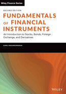
The profit diagram for a short futures position is also linear, but is downward sloping, as depicted in Figure 6.2.
In this case, the maximum profit occurs when the terminal futures price is zero and is equal in magnitude to the initial futures price. The maximum loss is obviously unlimited, because the terminal futures price has no upper bound. Thus holders of short positions, like investors who establish short positions in the spot market, are confronted with the prospect of finite profits but infinite losses. Quite obviously such investors too are bearish in nature, for they stand to make profits if the prices were to decline.
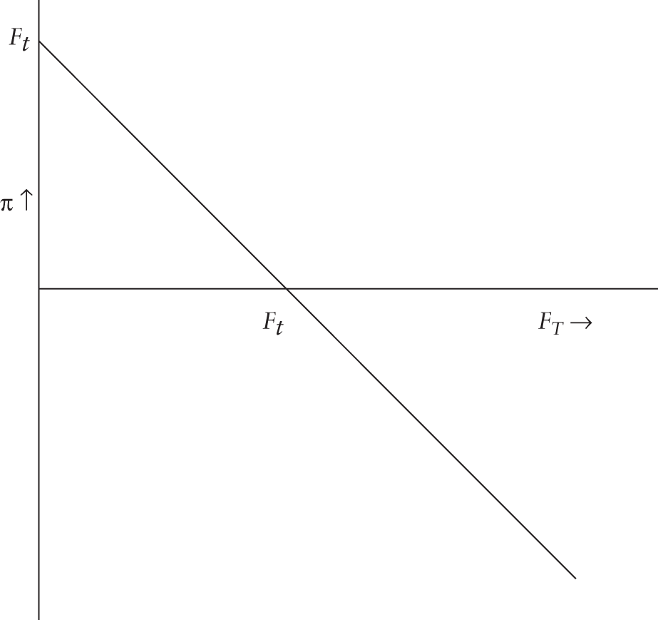
FIGURE 6.2 Profit Profile – Short Futures
VALUE AT RISK
To estimate the required margin, the clearinghouse needs to assess the potential loss for a party. Now, the loss from a futures contract does not arise all of a sudden but rather is accumulated over a period of time, as the futures price fluctuates from trade to trade in the market. In practice exchanges use a statistical technique known as Value at Risk (VaR) to estimate the potential loss over a given time horizon. The value at risk of a portfolio is an estimate of the loss over a specified time horizon for a given probability level. For instance, if the 95% value at risk of a portfolio over a one-day horizon is $7,500, it implies that there is only a 5% chance that the loss from the portfolio will exceed this amount over a one-day horizon. Quite obviously the estimate of the loss is a function of the specified probability level as well as the time horizon over which the loss is sought to be measured. That is, for a given probability level, the estimated loss over a three-day horizon will be different from the estimate for a one-day horizon. And, for a given time horizon the 95% VaR estimate will be different from the 99% VaR estimate. Consequently, a VaR number is meaningless until it is accompanied by the corresponding probability percentage and the time horizon. It must be remembered that the value at risk of a portfolio is not the maximum loss it can suffer over a given time period. In practice the value of a portfolio can always go to zero over any specified horizon, however small. Consequently, the maximum loss that a portfolio can suffer is its entire current value.
To illustrate how the VaR is computed in practice let us demonstrate the application of a method called RiskMetrics developed by JP Morgan. The volatility of the underlying asset on a given day is computed as an exponential moving average. The formula is given by:
σ is the value of the standard deviation or the volatility of the rate of return and r is the return for the day. In practice, a value of 0.94 is recommended for λ. Let us consider futures contracts on a stock index such as the S&P 500. The return for day t is defined as rt = ln(It/It−1), where It is the level of the index on day t. Consider a short futures position. We know that shorts will lose if the futures price were to rise. We can state with 99% confidence that the return will lie within +2.33 standard deviations. In practice, in order to account for the fat tails of the observed return distribution, a limit of +3 standard deviations is often taken. Thus, for a short position the upper limit is taken as +3σ.
Therefore

Hence if we know It, we can say with the stated level of confidence that the percentage change in the futures price will be less than or equal to ![]() .
.
Similar logic will show that the percentage decline in the futures price, which has pertinence for a long futures position, will be less than or equal to ![]() .
.
We will illustrate the application of this methodology with the help of an illustration.
THE EXPECTED SHORTFALL
The expected shortfall is the expected loss given that the loss exceeds the value at risk. The computation of the VaR and ES, given the distribution of losses for an investment, is given in Example 6.3.
SPOT-FUTURES EQUIVALENCE
Consider a futures contract that is entered into an instant prior to the specified delivery time. It is no different from a spot contract, as it requires the short to make delivery immediately and the long to accept immediate delivery. Thus, the futures price at the time of expiration of the contract must be exactly equal to the spot price, to preclude arbitrage. That is, as the time of expiration approaches, the spot and futures prices must converge with each other.
Let us examine the consequences if the futures price were not to be equivalent to the spot price at the time of contract expiration. There are two possibilities: the futures price may be higher or lower.
We will first consider the case where the futures price is higher. Assume that ABC is trading at $80 per share on the stock exchange and that ABC futures are trading at $82 on the futures exchange. Each futures contract is for 100 shares of stock.
Arbitrageurs will acquire 100 shares in the spot market and immediately go short in a futures contract. They can obviously take delivery at $80 in the spot market and simultaneously give delivery at $82 in the futures market. Thus, they have a costless assured profit of $2 per share or $200 per contract awaiting them. To preclude such an arbitrage opportunity, we require that the futures price must be less than or equal to the spot price at expiration.
The futures price, however, cannot be less than the spot price, for this situation too will give rise to an arbitrage opportunity. For instance, assume that the spot price of ABC is $80, while the futures price is $77.50. Arbitrageurs will short sell the stock and simultaneously go long in the futures contract. They will get $80 per share when they take the short position. They can immediately cover the short position by taking delivery under the futures contract at $77.50. Thus there is an arbitrage profit of $2.50 per share or $250 per contract. To rule out both forms of arbitrage it is imperative that the futures price converge to the spot price at the time of expiration.
PRODUCTS AND EXCHANGES
Futures contracts are available on a variety of financial assets and commodities. There was a time when the bulk of trading activity was in commodity-based products. Subsequently trading action has picked up considerably in contracts based on financial assets, such as stock indices, bonds, and foreign currencies, although many commodity derivative contracts continue to be very active. The newest derivatives on financial assets are single stock or individual stock futures.
Financial products on which contracts are traded include bonds such as T-notes and T-bonds, and money market securities such as Eurodollars. Contracts are traded on a variety of stock indices such as the Dow Jones Industrial Average, the Standard & Poor's 500, and the Nikkei 225. Foreign exchange products, based on the currencies of G-10 countries and of emerging markets, are also actively traded.
Derivative exchanges in the developed countries are characterized by large trading volumes for most of their products, and consequently attract attention from traders across the world. Emerging markets have picked up considerably in recent years, however, and offer attractive trading opportunities for both domestic market participants as well as cross-border traders. The derivatives markets have been characterized by a series of high-profile mergers in recent years. Prominent mergers include: CME with CBOT; NYSE with Euronext; NASDAQ with OMX; and BM&F with Bovespa.
CASH-AND-CARRY ARBITRAGE
An arbitrage strategy that is implemented for taking advantage of an overpriced futures contract is termed a cash-and-carry arbitrage. It entails the assumption of a long position in the spot market coupled with a short position in the futures market. If the futures contract is scheduled to expire immediately, the profit is FT − ST. But if there is time left for the maturity of the contract, the arbitrage profit may be expressed as ![]() where r is the interest rate for the period from t until T.1 The interest cost is the market rate of interest if the arbitrageurs are borrowing to fund the acquisition in the spot market; otherwise it is an opportunity cost if they are deploying their own funds.
where r is the interest rate for the period from t until T.1 The interest cost is the market rate of interest if the arbitrageurs are borrowing to fund the acquisition in the spot market; otherwise it is an opportunity cost if they are deploying their own funds.
REVERSE CASH-AND-CARRY ARBITRAGE
Such an arbitrage strategy comes into play when the futures contract is underpriced. It entails the assumption of a short position in the spot market coupled with a long position in the futures market. If the futures contract is slated to expire immediately, the profit is ST − FT. But if the maturity date of the contract is in the future, the profit may be expressed as ![]()
REPO AND REVERSE REPO RATES
Consider a cash-and-carry arbitrage strategy. It requires arbitrageurs to go long at a price St, in order for an assured payoff of Ft at the time of expiration. Thus the rate of return is given by

and is termed as the Implied Repo Rate (IRR). If the contract were to be fairly priced, then this rate will be exactly equal to the riskless rate. However, if the contract were to be overpriced, then this will exceed the riskless rate. Consequently, cash-and-carry arbitrage is profitable if the contract is overpriced, or equivalently if the IRR is greater than the borrowing rate.
Now let us consider reverse cash-and-carry arbitrage. The arbitrageurs will indulge in a short sale at a price St, knowing at the outset that they will eventually have to cover at a price Ft. Thus, their funding rate is

which is referred to as the Implied Reverse Repo Rate (IRRR). If the contract were to be fairly priced, then this rate will be exactly equal to the riskless rate. If the contract were to be underpriced, however, then this rate will be less than the riskless rate. Thus, reverse cash-and-carry arbitrage is profitable if the contract is underpriced or if the IRRR is less than the lending rate.
SYNTHETIC SECURITIES
Cash-and-carry arbitrage entails an initial investment in return for an assured payoff at the time of expiration of the futures contract. Thus, it is akin to an investment in a zero-coupon security such as a Treasury bill. Consequently, the artificial security created by such an arbitrage strategy is referred to as a synthetic T-bill. Quite obviously reverse cash-and-carry arbitrage is equivalent to a short position in a synthetic T-bill.
We can therefore state that: Spot – Futures = Synthetic T-bill
That is, a long position in the spot market, coupled with a short position in a futures contract, is equivalent to a long position in an artificial T-bill. Thus, if we have a natural position in any two of the three assets, then the third can be synthetically created.
VALUATION
The futures price is a function of the spot price, the interest rate, the time until expiration, and any payouts made by the underlying asset. We will start by analyzing the futures price of an asset that is not scheduled to make any payouts during the life of the contract.
We know that cash-and-carry arbitrage is ruled out if Ft ≤ St(1 + r), and that reverse cash-and-carry arbitrage is precluded if Ft ≥ St(1 + r). Hence, to rule out both forms of arbitrage it must be the case that Ft = St(1 + r) = St + rSt. Thus the futures price in an arbitrage-free setting should be equal to the cost of acquisition of the asset, and the funding cost for the duration of the contract. This relationship is referred to as the cost of carry. In Example 6.4 we show how the no-arbitrage futures price is determined.
THE CASE OF ASSETS MAKING PAYOUTS
Now assume that ABC is expected to make a payout of $2.50 after three months. Let us analyze the impact on both forms of arbitrage. Cash-and-carry arbitrage requires the trader to borrow and acquire the asset and go short in the futures contract. If the asset were to make a payout during the life of the contract, the effective carrying cost will stand reduced. The cost of funding the purchase of the security is rSt. If we denote the future value of the payout, as computed at the point of expiration of the futures contract by I, then the effective carrying cost is rSt − I. The reason why we need to compute the future value of the payout is the following. The interest cost is incurred at the point of expiration of the futures contract. In order to be consistent with the principles of time value of money, the magnitude of the payout too should be measured at this point. If the payout has occurred prior to the expiration date of the contract, it will obviously need to be compounded until the point of expiration. Thus, to rule out cash-and-carry arbitrage we require that Ft ≤ St × (1 + r) − I.
Now let us analyze reverse cash-and-carry arbitrage. The arbitrageur would have short sold the asset and invested it in the market, while simultaneously going long in the futures contract. The income from the investment proceeds of the short sale is rSt. However, if there were to be a payout from the asset, then the interest income will stand reduced, because the short seller, as explained earlier, will have to compensate the party who is lending the asset for any lost income. Thus, the net proceeds from the investment is rSt − I. Thus, to rule out reverse cash-and-carry arbitrage we require that
Hence to rule out both forms of arbitrage in the case of contracts on assets that make a payout, we require that Ft = St × (1 + r) − I. Here are numerical illustrations of how arbitrage profits can be earned if this condition is violated.
PHYSICAL ASSETS
Unlike financial assets, physical assets do not make payouts; however, the acquirers of such assets have to expend resources for storing and possibly insuring such assets. Let us denote the total cost incurred in holding such assets by Z. A cost is nothing but a negative income. Thus, if we replace the variable I in the pricing equation for assets making a payout with Z, we get the relationship for physical assets that is
And yet the issue is not so straightforward. First we need to make a distinction between assets that are held for the purpose of investment and those that are held for consumption purposes. This has implications for the ability to short sell the asset. Financial assets such as stocks and bonds are held for investment reasons. Holders of such assets will have no problems in lending such assets to facilitate a short sale, if the asset is returned at the end of the period for which they intend to hold it, and if they are compensated for any income that they would have received had they continued to hold it. Precious metals like gold and silver are also usually held for investment purposes. An agricultural product like wheat or corn, however, may be held for other reasons. A wheat mill owner may choose to hold it in stock to avoid problems of short supply due to unanticipated events such as a natural calamity or a rainfall failure. Such assets will in these circumstances not be parted with to facilitate short sales. We term such assets as consumption or convenience assets and say that the holders are receiving a convenience value. The convenience value is like an implicit dividend; however, it cannot be quantified for (1) it cannot be objectively measured, and (2) it varies from holder to holder. Before we proceed to discuss the pricing of futures contracts on physical assets let us introduce the concept of quasi-arbitrage.
We know that a long spot position plus a short futures position is equivalent to a long position in a T-bill-like security, which we have termed as a synthetic T-bill. The variables can be repositioned to show that a synthetic position in any of the three products – the underlying asset, the futures contract, or the riskless asset – can be taken if we have natural positions in the remaining assets. A strategy that is designed to take a synthetic position in a product, because the perceived returns are greater than what traders would get were they to take a natural position in it, is termed as a quasi-arbitrage strategy.
Let us now consider cash-and-carry arbitrage. It requires traders to go long in spot and short in futures. This per se should pose no problems irrespective of whether the asset is a pure asset, like gold or silver, or a convenience asset, like wheat. Thus, overpricing of the futures contract is ruled out; however, the reverse cash-and-carry argument may be needed to be supplanted with a quasi-arbitrage argument to rule out an underpriced futures contract, as the following illustration will demonstrate.
Take the case of a party who already owns an ounce of the metal. They can sell it for $250 and invest the proceeds at 8% per annum for six months. Simultaneously they can go long in a futures contract. At the end of six months the asset will be back in their possession, and they would have saved $10 in the process by way of saving of storage costs. Thus, quasi-arbitrage is indeed a profitable activity in such circumstances, and a combination of conventional cash-and-carry arbitrage and reverse cash-and-carry quasi-arbitrage will ensure that the asset is neither underpriced nor overpriced.
The situation can be different, however, in the case of a convenience asset. Conventional cash-and-carry arbitrage will help ensure that the contract is not overpriced. Traders may be unwilling to indulge in either reverse cash-and-carry arbitrage or quasi-arbitrage because they are getting a convenience value from the asset. Thus, all that we can state in the case of such assets is that Ft ≤ St × (1 + r) + Z. That is, while the contract cannot be overpriced, what looks like underpricing may not be exploitable in practice.
NET CARRY
The net carry for an asset that makes no payouts may be expressed as NC = r, while for assets making a payout it is ![]() . For assets that entail the payment of storage costs we can express it as
. For assets that entail the payment of storage costs we can express it as ![]() . Thus, in all cases we can state that Ft = St × (1 + NC). If, however, the asset were to yield a convenience value, we can state the futures price as: Ft = St × (1 + NC) − Y. Y, the variable that equates the two sides, is termed as the marginal convenience value.
. Thus, in all cases we can state that Ft = St × (1 + NC). If, however, the asset were to yield a convenience value, we can state the futures price as: Ft = St × (1 + NC) − Y. Y, the variable that equates the two sides, is termed as the marginal convenience value.
BACKWARDATION AND CONTANGO
If the futures price is in excess of the spot price, or if the price of the nearby futures contract is lower than that of the more distant contract, then we say that the market is in contango. If, however, the futures price is less than the spot price, or if the nearby contract is priced higher than the more distant contract, then we say that the market is in backwardation. Let us first consider financial assets.
The net carry may be positive or negative, depending on whether the interest cost dominates the income from the security, or is dominated by it. Thus, the market may be in backwardation or in contango.
For physical assets held for investment purposes, the net carry will always be positive. Consequently, such assets will always be in contango. Convenience assets may be in backwardation or in contango. For such assets:
The net carry will be positive. If the effect of the net carry were to dominate, the market will be in contango. However, if the convenience yield is substantial, then the market may be in backwardation. Tables 6.4 and 6.5 represent two illustrations showing markets in backwardation and contango respectively. In practice it is not necessary that a market should steadily be in backwardation or in contango. For instance, while a three-month contract may be priced higher than the spot, which is what we would associate with a contango market, a six-month contract may be priced lower than the three-month contract, thereby displaying backwardation.
TABLE 6.4 Illustration of a Contango Market
| Contract | Price |
|---|---|
| Spot | $100.00 |
| 3-M Futures | $107.50 |
| 6-M Futures | $112.50 |
| 9-M Futures | $118.00 |
| 12-M Futures | $122.00 |
TABLE 6.5 Illustration of a Backwardation Market
| Contract | Price |
|---|---|
| Spot | $100.00 |
| 3-M Futures | $ 97.50 |
| 6-M Futures | $ 92.50 |
| 9-M Futures | $ 88.00 |
| 12-M Futures | $ 82.00 |
THE CASE OF MULTIPLE DELIVERABLE GRADES
We have shown that the futures price must converge to the spot price of the underlying asset. But in the case of contracts on certain commodities, multiple grades are permitted for delivery. The question in this case is, which spot price will the futures price converge to, as each eligible grade of the underlying asset will have its own spot price?
Before we go on to answer this question, let us deal with the issue of the spot-futures ratio. In the case of contracts where there is only one eligible grade for delivery, any arbitrage strategy that entails the assumption of a futures position until the time of expiration requires spot-futures positions in the ratio of 1:1. That is, the number of units in which a long or a short position is taken in the spot market must be identical to the number of units of the underlying asset represented by the position taken in the futures market. If multiple grades are permitted for delivery, however, then this will typically not be the case. There are two possible ways of price compensation when multiple grades have been specified for delivery. These are referred to as multiplicative price adjustment and additive price adjustment respectively.
In the case of contracts where a multiplicative price adjustment system has been specified, the short will receive aiFT if he were to deliver grade ‘I’ where ai is the adjustment factor for the grade. One grade will be designated as the par grade, for which the adjustment factor will be 1.0. For premium grades the adjustment factor will be greater than 1.0, while for discount grades it will be less than one. The cash inflow for an arbitrageur who chooses to initiate a cash-and-carry arbitrage strategy at time t with a short position in ‘h’ futures contracts will be aiFT + h(Ft − FT). To make the cash flow from this strategy riskless we need to eliminate the term involving ‘T,’ which implies that h = ai. Thus, the number of futures contracts required is equal to the adjustment factor of the grade in which the trader has taken a long spot position.
The profit from the arbitrage strategy is aiFt − St(1 + r). To rule out arbitrage we require that the profit be zero, which implies that ![]() . Because there are multiple grades, this condition clearly cannot prevail for all grades simultaneously. The most preferred grade for which this condition will prevail is called the cheapest to deliver grade (CTD). In technical terms, we say that the futures price prior to expiration will be equal to the delivery-adjusted no-arbitrage futures price of the CTD grade, where the no-arbitrage futures price is St × (1 + r). For all the other grades, which we will denote in general by ‘j,’ it must be the case that
. Because there are multiple grades, this condition clearly cannot prevail for all grades simultaneously. The most preferred grade for which this condition will prevail is called the cheapest to deliver grade (CTD). In technical terms, we say that the futures price prior to expiration will be equal to the delivery-adjusted no-arbitrage futures price of the CTD grade, where the no-arbitrage futures price is St × (1 + r). For all the other grades, which we will denote in general by ‘j,’ it must be the case that ![]() . The no-arbitrage condition at expiration is obviously FT = ST/ai. Thus, the futures price will converge at the time of expiration of the contract to the delivery-adjusted spot price of the CTD grade where the delivery-adjusted spot price of a grade is S/a. For all the other grades ‘j,’ the delivery-adjusted spot price will obviously be higher. Thus, the CTD grade at expiration is the grade with the lowest delivery-adjusted spot price.
. The no-arbitrage condition at expiration is obviously FT = ST/ai. Thus, the futures price will converge at the time of expiration of the contract to the delivery-adjusted spot price of the CTD grade where the delivery-adjusted spot price of a grade is S/a. For all the other grades ‘j,’ the delivery-adjusted spot price will obviously be higher. Thus, the CTD grade at expiration is the grade with the lowest delivery-adjusted spot price.
The multiplicative system of price adjustment is used for contracts like Treasury Bond futures. Consider the September 2018 futures contract. The CTD bond is a 5% coupon bond maturing on 15 May 2047. Its adjustment factor is 0.8642.
On September 15, which is an allowable date for delivery, the futures price (per dollar 100 of face value) is 96-08. The accrued interest per $100 of face value is $1.6984. Thus, the price payable by the long is:
Now let us consider the system of additive price adjustment, which is used for contracts on agricultural commodities with multiple deliverable grades. In the case of such contracts, the short will receive FT + ai, if he were to deliver grade i where ai is the adjustment factor for the grade. One grade will be designated as the par grade for which the adjustment factor will be 0.0. For premium grades the adjustment factor will be positive, while for discount grades it will be negative. The cash inflow for an arbitrageur who chooses to initiate a cash-and-carry arbitrage strategy at time t with a short position in ‘h’ futures contracts will be FT + ai+ h(Ft − FT). To make the cash flow from this strategy riskless we need to eliminate the term involving ‘T,’ which implies that h = 1. Thus the appropriate spot-futures ratio for such contracts is 1:1, as it is for contracts that do not offer a choice with respect to the eligible grade.
The profit from the arbitrage strategy is Ft + ai − St(1 + r). To rule out arbitrage we require that the profit be zero, which implies that ![]() . As there are multiple grades, this condition once again cannot prevail for all grades simultaneously. The most preferred grade for which this condition will prevail is called the cheapest to deliver grade (CTD). Thus, as in the case of multiplicative adjustment, the futures price prior to expiration will be equal to the delivery-adjusted no-arbitrage futures price of the CTD grade, where the no-arbitrage futures price is St × (1 + r). For all the other grades, which we will denote in general by ‘j,’ it must be the case that
. As there are multiple grades, this condition once again cannot prevail for all grades simultaneously. The most preferred grade for which this condition will prevail is called the cheapest to deliver grade (CTD). Thus, as in the case of multiplicative adjustment, the futures price prior to expiration will be equal to the delivery-adjusted no-arbitrage futures price of the CTD grade, where the no-arbitrage futures price is St × (1 + r). For all the other grades, which we will denote in general by ‘j,’ it must be the case that ![]() . The no-arbitrage condition at expiration is FT = St − ai. Thus, the futures price will converge at the time of expiration of the contract to the delivery-adjusted spot price of the CTD grade where the delivery-adjusted spot price of a grade is S − a. For all the other grades ‘j,’ the delivery-adjusted spot price will obviously be higher. Thus, the CTD grade at expiration is once again the grade with the lowest delivery-adjusted spot price.
. The no-arbitrage condition at expiration is FT = St − ai. Thus, the futures price will converge at the time of expiration of the contract to the delivery-adjusted spot price of the CTD grade where the delivery-adjusted spot price of a grade is S − a. For all the other grades ‘j,’ the delivery-adjusted spot price will obviously be higher. Thus, the CTD grade at expiration is once again the grade with the lowest delivery-adjusted spot price.
RISK ARBITRAGE
In the preceding case we stated that the futures price prior to expiration will converge to the delivery-adjusted no-arbitrage futures price of the CTD grade. For all other grades we can state that ![]() or
or ![]() . The issue is that if the futures price is lower than the delivery-adjusted no-arbitrage futures price for a grade, then why can we not implement a reverse cash-and-carry arbitrage strategy to earn a costless, riskless profit. The answer is that such strategies are not riskless.
. The issue is that if the futures price is lower than the delivery-adjusted no-arbitrage futures price for a grade, then why can we not implement a reverse cash-and-carry arbitrage strategy to earn a costless, riskless profit. The answer is that such strategies are not riskless.
Let us analyze the cash-and-carry strategy for contracts on a commodity where the additive/multiplicative price adjustment systems are used. Arbitrageurs would have gone long in the required number of units in the spot market and assumed a short position in the futures market. Since they hold the short position in futures, they have the prerogative to decide as to which grade they should choose to deliver. If the maximum profit is likely to be obtained by delivering the grade in their possession, then they will choose to deliver that grade. If, however, they were of the opinion that any other grade is likely to lead to a larger cash flow if delivered, then they would choose to dispose of the grade in their possession in the spot market and acquire the required number of units of the grade that will lead to optimal profits if delivered. Consequently, while arbitrageurs may realize the profits that they have been anticipating from the outset, they can only earn more if circumstances were to change.
Reverse cash-and-carry arbitrage, however, is different. It requires arbitrageurs to go long in futures and short in the spot. In this case the right to choose the deliverable grade is with the counterparty and not the arbitrageurs. There is no guarantee that the counterparty will choose to deliver the grade that the arbitrageur has sold short. If they choose to deliver a different grade because it is optimal for them, then the arbitrageurs will realize a lower profit than anticipated. Thus, while implementing a reverse cash-and-carry strategy, arbitrageurs may end up realizing a lower profit, which in practice may even be a loss, and can never earn more than what they were anticipating at the outset. It is for this reason that reverse cash-and-carry arbitrage under such circumstances is termed as risk arbitrage. We will now demonstrate these arguments, first with the multiplicative adjustment system, and then with the additive adjustment system.
THE CASE OF MULTIPLICATIVE ADJUSTMENT
Consider the case of arbitrageurs who have gone long in one unit of grade ‘i’ of the asset and short in ai futures contracts. Assume that at the point of expiration, another grade ‘j’ has become more profitable to deliver. If so, they will sell the unit of grade ‘i’ that they possess in the spot market and acquire ai units of grade ‘j’ to satisfy their delivery commitments under the futures contract. Let us consider their cash flows.
Inflow from sale of grade ‘i’ = Si,T
Marking to market profit/loss = ai(Ft − FT)
Cost of acquisition of grade ‘j’ = aiSj,T
Inflow from delivery under the futures contract = ai × ajFT

We have used the fact that ajFT = Sj,T and that ‘j’ is the CTD grade and so ![]() .
.
Thus the arbitrageurs will never earn a profit that is less than what they anticipated at the outset.
Now let us turn to reverse cash-and-carry arbitrage. It would have been initiated by short selling one unit of grade “i” and going long in ai futures contracts. Assume that at the point of expiration, another grade “j” has become more profitable to deliver. If so, the arbitrageurs will acquire one unit of grade “i” to cover their short position and sell ai units of grade “j” which they would receive under the futures contract in the spot market. Let us consider their cash flows.
Outflow on account of acquisition of grade “i” = Si,T
Marking to market profit/loss = ai(FT − Ft)
Proceeds from sale of grade “j” = aiSj,T
Outflow due to acquisition under the futures contract = ai × ajFT
We know that ![]() . Thus, the net outflow can be greater than what was anticipated at the outset but not less. Thus, reverse cash-and-carry arbitrage is fraught with danger and is consequently termed as risk arbitrage.
. Thus, the net outflow can be greater than what was anticipated at the outset but not less. Thus, reverse cash-and-carry arbitrage is fraught with danger and is consequently termed as risk arbitrage.
THE CASE OF ADDITIVE ADJUSTMENT
Consider the case of cash-and-carry arbitrage. That is, the arbitrageurs have gone long in one unit of grade ‘i’ of the asset and short in one futures contract. Assume that at the point of expiration, another grade ‘j’ has become more profitable to deliver, and that consequently they decide to sell their unit of grade ‘i’ in the spot market and acquire one unit of grade ‘j’ to satisfy their delivery commitments under the futures contract. Let us consider their cash flows.
Inflow from sale of grade ‘i’ = Si,T
Marking to market profit/loss = (Ft − FT)
Cost of acquisition of grade ‘j’ = Sj,T
Inflow from delivery under the futures contract = FT + aj
The net cash flow = Si,T + FT + aj+ (Ft − FT) − Sj,T
= Ft + ai + [Si,T − ai − (Sj,T − aj)]
Because grade ‘j’ is the CTD, we know that (Si,T − ai) > (Sj,T − aj). Thus, the net inflow may be higher than anticipated but never less. Using similar arguments, we can demonstrate that reverse cash-and-carry arbitrage in the case of a contract for which additive adjustment has been prescribed is also a case of risk arbitrage.
TRADING VOLUME AND OPEN INTEREST
Trading volume refers to the number of contracts traded during a given time interval. In practice we are usually concerned with the volume for a given trading day that is from the commencement of trading in the morning until the close of the market. Every trade that is consummated during the day adds to the trading volume for that day. Take the case of Mitch, who goes long in 250 contracts on wheat with Doug. The addition to the trading volume for the day is obviously +250. A trade will always serve to increase the observed volume for the time period.
Open interest refers to the number of open positions at any point in time. Every long position must be matched by a corresponding short position. Consequently, open interest may be measured as the total number of open long positions at a given point in time, or equivalently as the total number of open short positions. A trade may lead to an increase or a decrease in the open interest or may leave it unchanged as we will demonstrate.
Assume that Mitch took a long position in 250 contracts on wheat last week and that Doug also had a prior short position in 200 contracts on the commodity. The two parties now execute a trade in 100 contracts wherein Mitch takes a long position and Doug takes a short position. The number of open long positions increases by 100 as a consequence of the trade. Equivalently the number of open short positions also increases by 100. Thus, the impact of the trade is to increase the open interest by 100 contracts. Hence if a trade results in an establishment of new positions by both the parties who enter into it, the open interest will rise.
Now consider a situation where Mitch goes long in 100 contracts with Kirk, who takes a short position. Assume that Kirk previously had a long position in 200 contracts. The impact of the trade is to increase the number of total open long positions by 100 as seen from Mitch's perspective; however, the trade simultaneously results in a decline of the open interest by 100 contracts since Kirk is partially offsetting his position. Thus, the net impact on open interest is nil. So, if a trade results in the opening of a position by a party by trading with a counterparty who is offsetting, the open interest will remain unchanged.
Finally, consider a situation where Mitch takes a short position in 100 contracts by trading with Doug, who takes a long position. The consequence of the trade is that Mitch's long position is reduced by 100 contracts. Simultaneously the trade has resulted in a decrease of 100 in Doug's short position. Thus, the open interest will decline by 100 contracts in this case. Therefore, if a trade results in the offsetting of existing positions by both the parties, open interest will decline.
Thus, while a trade will always lead to an increase in the trading volume for a day, its impact on the open interest will depend on the prior positions held by the counterparties.
A high trading volume for a day is symptomatic of a highly liquid market. Open interest, on the other hand, is an indicator of high future liquidity, because the higher the open interest, the greater is the potential for offsetting transactions.
DELIVERY
Both forward and futures contracts may set forth terms for delivery, but the two types of contracts differ in several respects. First, the majority of forward contracts that come into existence are actually settled by delivery. On the other hand, the majority of futures contracts are offset prior to maturity. In practice, a small number of futures contracts, ranging from 2 to 5%, are actually settled by delivery.
Second, in the case of a forward contract the party who went short at the outset will end up delivering to the party with whom they traded initially. As explained earlier, there is no intervention in the case of such contracts by an agency such as a clearinghouse, and consequently the link between the two original counterparties very much remains intact. In the case of a futures contract, however, the link between the two counterparties is snapped by the clearinghouse immediately after the trade. Subsequently one or both counterparties may exit the market by taking a counterposition. Hence, when a short expresses the desire to make delivery, the exchange has to locate a party to whom they can deliver. In practice the long who is chosen to accept delivery is the party with the oldest outstanding long position.
Third, futures contracts are marked to market on a daily basis. The cash flow, for a long position, on a given day is Ft − Ft−1. If we aggregate the cash flows, we get  . In order to ensure that the price paid by the long is what was contracted at the outset, they should pay a price P, such that after accounting for the cash flows from marking to market they effectively end up paying F0.
Thus, the price at which delivery is made under a futures contract is the terminal futures price, which, as we have seen earlier, is no different from the terminal spot price.
In the case of a forward contract, however, there is no marking to market. Hence the price that is paid by the long at the time of delivery is the price that was contracted at the outset.
CASH SETTLEMENT
All futures contracts do not mandate the delivery of the underlying asset. Stock index futures contracts, for instance, do not, for it is extremely cumbersome to deliver a large basket of securities (the S&P 500 is composed of 500 stocks) in exactly the same proportions as they are present in the index. Contracts such as index futures are cash settled. That is, they are marked to market one last time at the close of trading on the expiration day, and all positions are declared closed. Both the long and the short will exit the market with their profit/loss, but without taking delivery. The cash flow for the long will be Ft − F0, while that for the short will be F0 − Ft. Cash settlement may at times be the prescribed mechanism in markets where there is a perceptible risk of manipulation or the potential to create artificial shortages. Exchanges in many developing economies therefore prescribe cash settlement as the norm for many contracts.
HEDGING AND SPECULATION
There are two categories of traders in futures contracts: hedgers and speculators. The former take positions in futures contracts to reduce or eliminate their exposure to risk on account of a spot market position. The latter consciously seek to take an exposure to risk in the futures market in anticipation of gains.
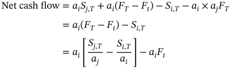
The rationale for hedging may be explained as follows. Take the case of traders who own 5,000 bushels of wheat they are planning to sell after a month. Their worry is that the price of the product may fall in the spot market by the time the delivery date arrives. They can, however, go short in a futures contract at the prevailing futures price Ft. If so, they can be assured of being able to sell at this price, no matter what the spot price of wheat may be on the expiration date of the contract. In this argument we are assuming that the planned date of sale of the commodity coincides with the expiration date of the futures contract. In practice this may not be the case. If the wheat were to be sold before the delivery date of the contract on a date t*, the traders would have to sell the asset in the spot market at a price St*, and collect their profit/loss from marking to market in the futures market. The net inflow will be:
![]() is referred to as the basis. Thus, the risk for the hedger is the risk of variation in the basis. If the trader had not hedged, he would have received
is referred to as the basis. Thus, the risk for the hedger is the risk of variation in the basis. If the trader had not hedged, he would have received ![]() . The risk of variation in the spot price is termed as price risk. Hence hedging replaces price risk with the more acceptable risk of variation in the price difference between the spot and the futures price, which is termed as basis risk.
. The risk of variation in the spot price is termed as price risk. Hence hedging replaces price risk with the more acceptable risk of variation in the price difference between the spot and the futures price, which is termed as basis risk.
Now let us take the case of traders who are short in the spot market. The term connotes that they have a prior commitment to buy. For instance, a company in Bangalore may have imported mainframe computers from the United States and may have a commitment to pay in USD after a month. The risk is that the rupee price of the US dollar may rise or, in other words, that the US dollar may appreciate. Such traders can go long in the futures market in order to hedge. If the date of acquisition of dollars were to coincide with the expiration date of the futures contracts, the dollars can be acquired at the initial futures price Ft. If not, the dollars can be bought in the spot market, and the profit/loss from marking to market can be collected. In this case, the outflow will be:
The magnitude of the cash inflow for a short hedger is Ft + ![]() , while the magnitude of the outflow for a long hedger is also Ft +
, while the magnitude of the outflow for a long hedger is also Ft + ![]() . The short hedger therefore stands to benefit from a rising basis, while the long hedger stands to profit from a falling basis. We know that traders with short futures positions stand to benefit from falling futures prices while those with long futures positions stand to gain from rising futures prices. The basis itself may be construed as a price, for it is but the difference of two prices, or a synthetic price. Consequently, we say that the short hedger is long the basis while the long hedger is short the basis.
. The short hedger therefore stands to benefit from a rising basis, while the long hedger stands to profit from a falling basis. We know that traders with short futures positions stand to benefit from falling futures prices while those with long futures positions stand to gain from rising futures prices. The basis itself may be construed as a price, for it is but the difference of two prices, or a synthetic price. Consequently, we say that the short hedger is long the basis while the long hedger is short the basis.
On the day of expiration, the basis will be zero, for bT = ST − FT = 0, because the futures price must converge to the spot price when the contract itself is scheduled to expire. A hedge without any inherent basis risk is termed as a perfect hedge. Thus, one of the key requirements for a perfect hedge is that the date of termination of the hedge must coincide with the expiration date of the futures contract. In the case of a perfect hedge a short hedger can be assured of receiving the futures price that was prevailing when the hedge was set up, while a long hedger can be guaranteed that he can acquire the asset by paying the futures price that was prevailing when he took a long position.
There is another key requirement for a perfect hedge. Let us consider the cash inflow for a short hedger, who is long in Q units of the asset and short in N futures contracts where each contract is for C units of the underlying asset. Thus the futures position represents Qf units of the underlying asset, where Qf = NC. The cash inflow is: QST + NC(Ft − FT). For this to be equal to QFt, we require that Q = NC = Qf. Thus the hedge ratio must be 1:1, which implies that the quantity being hedged must be an integer multiple of the size of the futures contract.
Let us summarize the conditions for a perfect hedge.
- The first and the most basic condition is that futures contracts must be available on the asset whose price is being sought to be hedged.
- The date of sale/purchase of the underlying asset must coincide with the expiration date of the futures contract.
- The number of units of the underlying asset must be an integer multiple of the contract size.
In practice, condition-1 is likely to be satisfied in many cases; however, condition-2 is not. Take, for instance, a commodity on which contracts expiring in March, May, July, September, and December are available. Assume that the contracts expire on the 21st of the respective months, whereas the hedger would like to terminate the hedge on the 15th of July. The May contract is not appropriate as it will leave the trader open to price risk for the period from May until July. July contracts are not usually suitable because futures contracts can exhibit erratic price movements in the expiration month. Consequently, a hedger who seeks to buy or sell in July would like to avoid exposure to this contract. Thus, the choice is between the September and December contracts. In practice, the further away the expiration month, the greater is the basis risk. The reason is as follows.
The spot price, as well as the futures price, is being influenced by the same economic factors. The spot price represents the current market price, whereas the futures price is the price for a transaction at a future point in time. If the termination date of the hedge is close to the expiration date of the futures contract, then both the markets will be discovering the price of the product for virtually the same point in time. Consequently, the prices will converge such that the difference or the basis is more predictable.2 Consequently the September contract is likely to expose the trader to a lower basis risk than the December contract. Hence in practice, when the transaction date does not coincide with the expiration date of the futures contract, the hedger will choose a contract which is slated to expire soon after the month in which the hedge is being terminated.
ROLLING A HEDGE
In the preceding argument we assumed that the hedger would choose the September futures contract. Let us assume that the futures position was taken on 21 April. On that day, however, the September contracts may not have commenced trading. Or they may be so illiquid as to deter investors who seek to enter and exit the market at a price that is close to the true or fair value of the asset. In such cases, it is conceivable that hedgers will first go short in the May contract. Since they would like to avoid exposure to the contract in its expiration month, they are likely to offset the position at the end of April and go short in July contracts. Finally, toward the end of June, they are likely to offset the July contracts and take a short position in September contracts. On 15 July they will sell the underlying asset in the spot market and offset the September futures position. Such a hedging strategy is known as a rolling hedge.
TAILING A HEDGE
Consider a perfect hedge. We know that a short hedger will receive the spot price prevailing at the time of termination of the hedge, and then collect the total profit/loss from marking to market. The profit/loss from marking to market on a given day ‘t’ is Ft−1 − Ft. This can be reinvested if it is a profit, or financed if it is a loss, until the maturity date so as to yield (Ft−1 − Ft)(1 + r)t*−t. The cumulative profit/loss from a futures position equivalent to Qf units is  . This will in general not be equal to Qf[F0 −
 ![]() ]. To make it so, we should have a position in
]. To make it so, we should have a position in

futures contracts at the beginning of day ‘t.’ Thus, we would have to start with a quantity less than Qf and increase our position steadily at the end of each day. Consequently, if we were to start with Qf units rights from the outset, we would be overhedging. Overhedging will inflate the profit when there is a profit but will magnify the loss when there is a loss. The process of periodically adjusting the futures position in order to account for the effect of marking to market is termed as tailing. In practice the futures position is not usually adjusted daily but only periodically, for each adjustment entails the incurrence of transactions costs.
THE MINIMUM VARIANCE HEDGE RATIO
We know that the cash flow for a short hedger is:
If t* = T, then ![]() = ST =
= ST = ![]() = FT, and we should set Qf = Q such that the total revenue is QFt, an amount about which there is no uncertainty. Thus, in order to obtain a perfect hedge under such circumstances, we need to set Qf = Q, or in other words we need a hedge ratio of 1:1.
= FT, and we should set Qf = Q such that the total revenue is QFt, an amount about which there is no uncertainty. Thus, in order to obtain a perfect hedge under such circumstances, we need to set Qf = Q, or in other words we need a hedge ratio of 1:1.
In general, however, the revenue from the hedged position is:
where h is obviously the hedge ratio.
At the outset, we know Q, St, and h. In order to minimize risk we need to minimize the variance of the revenue using the only variable in our control, which is h.

Let us denote Var(ΔS) by σs2 and Var(ΔF) by σf2. The correlation between the two variables is ρ. If we minimize the variance of R with respect to h, we get ![]() .
.
ESTIMATION OF THE HEDGE RATIO AND THE HEDGING EFFECTIVENESS
Consider the following statistical relationship.
To estimate the parameters, we can run a linear regression with ΔF as the independent variable and ΔS as the dependent variable. The minimum variance hedge ratio is given by the slope coefficient β. The R2 of the regression is a measure of the hedging effectiveness. If the basis risk is equal to the price risk, there will be no risk reduction and the R2 will be zero. However, if there is a perfect hedge, then the R2 will be 1.0. Thus, in practice we will get a value between 0 and 1.0.
CROSS-HEDGING
Sometimes it may so happen that there are no suitable futures contracts on the product whose price is sought to be hedged. It could be because there is no contract on the commodity in which we are interested. Otherwise, it could be the case that while contracts are available, they are so illiquid that the hedger does not have the confidence to take a position. Under such circumstances, the trader may choose to hedge by taking a futures position in a closely related commodity, where, by the term closely related, we mean a commodity whose price is highly positively correlated with that of the commodity that we are interested in. The use of futures contracts on a closely related commodity is termed as cross-hedging.
- The revenue for the short hedger under such circumstances is: St* + [F*t − F*t*], where S and F represent the spot and futures prices of the commodity the revenue from which is sought to be hedged, and S* and F* are the spot and futures prices of the closely related commodity that is being used for cross-hedging.
- This can be expressed as F*t + (S*t* − F*t*) + (St* − S*t*). The basis therefore consists of two components. (S*t* − F*t*) is the basis if the asset being hedged is the same as the asset underlying the futures contract. The second term, (St* − S*t*), is the basis that arises due to the fact that the two assets are different. If t* = T, then the first term will drop out and the basis for a cross-hedge will be (St* − S*t*).
SPECULATION
Futures contracts can be used for speculation. Take the case of traders who are bullish about the market. If so, they can go long in a futures contract at the prevailing spot price. If the market were to rise, they can either take delivery at expiration and sell the commodity at the prevailing spot price, which by assumption is higher, or they can offset their position prior to expiration and exit the market with a cumulative profit from marking to market.
LEVERAGE
Bulls have a choice between a long spot position and a long futures position from the standpoint of speculation, whereas bears have a choice between a short spot position and a short futures position.
Futures positions offer the benefit of leverage to a speculator. As we have seen earlier, a position may be said to be levered if a small price movement in the underlying asset has a disproportionately large impact on the rate of return.
Why do we say that a futures position is levered? Take the case of a trader who goes long in a futures contract on a commodity by depositing $5,000 as the initial margin. Let the initial futures price be $5.00 per bushel and assume that the contract size is 5,000 bushels. Consider a price increase of $0.40 per bushel. The profit per contract will be $2,000, which amounts to a return of 40% on the initial margin deposit. If the trader had taken a spot position at a price equal to the initial futures price, however, the investment would have been $25,000, and a profit of $2,000 would amount to a return of only 8%. Thus, the leverage inherent in a futures contract helps magnify the rate of return. However, as we are aware, leverage is a double-edged sword. That is, losses if any will also be magnified. A price decline of $0.40 per bushel would amount to a –40% return on the futures position, but to a loss of only 8% on a spot position.
CONTRACT VALUE
When a forward contract is entered into, neither the short nor the long has to pay a price to enter into it. The price at which the underlying asset is scheduled to be bought/sold at a future date as per the contract is referred to as the delivery price of the contract. The delivery price is set in such a way that the contract value at inception is zero. That is, the two equal and offsetting obligations ensure that neither party has to pay the other to take a position.
The delivery price remains fixed once a contract is sealed. However, the price for a fresh contract will keep fluctuating over time. The price that is applicable if a forward contract were to be sealed at a particular instant is referred to as the forward price. If a contract were to be sealed, the prevailing forward price will be the delivery price of the contract. But an instant later the forward price will typically change.
Although the value of a contract will be zero at inception, such contracts will accrue value as time elapses. Consider a long forward position taken at a point of time in the past, when the forward price was K. This forward price would have been set as the delivery price of the contract. Now, a few periods later, the prevailing forward price is F. If the party who had originally gone long were to offset, they would have to do so by going short at a price F. The two offsetting positions would lead to a cash flow of F − K at the time of expiration of the contract. The current value of the contract is the present value of this cash flow. As we have seen earlier, rising prices will lead to profits for the longs, while falling prices will lead to losses. Thus, if the forward price at a point in time were to be higher than the delivery price of the contract, a long forward position will have a positive value. If the price were to have declined after a contract was entered into, however, a long position will have a negative value. The situation will be exactly the opposite for shorts. Falling prices will lead to positive contract values while rising prices will lead to negative values. Example 6.17 shows how to compute the value of a preexisting forward contract.
What about the value of a futures contract? Such contracts too will have a zero value at inception. At the end of each day, starting with the trade date, the contract will be marked to market. Marking to market is nothing but the settlement of built-up value since the time that the contract was previously marked to market. The party with a positive value will have their margin account credited while the counterparty's margin account will be debited. Thus, the only time that a futures contract acquires value is in the intervening period between two successive marking to market dates. Each time the contract is marked to market, the value will revert back to zero.
FORWARD VERSUS FUTURES PRICES
In general, the forward price will not be equal to the futures price for contracts on the same underlying asset and with the same expiration date. The reason is that futures contracts are periodically marked to market, while forward contracts are not.
It can be shown that if the interest rate is a constant and is equal for all maturity periods, then there will be no difference between the forward price and the futures price. In reality, however, interest rates are a random variable; that is, they are stochastic in nature. Therefore, in practice the forward price will differ from the futures price.
The rationale is the following. If interest rates were to be positively correlated with futures prices, rising prices will lead to a situation where the long, who will have a profit under such circumstances, can invest profits from marking to market at high rates of interest. Clearly, falling futures prices will lead to a situation where the longs have to finance their losses at a lower rate of interest. Thus, an interest rate that is positively correlated with futures prices is beneficial for the longs. Therefore, longs will have to pay more under such circumstances, which means that the futures price will be higher than the forward price. The positive correlation has no consequences for a forward contract since there is no concept of marking to market. Thus, under such circumstances, futures prices will be higher than forward prices.
On the other hand, if futures prices were negatively correlated with interest rates, then rising futures prices would correspond to a situation where the longs are investing their profits at lower rates of interest, while declining prices will obviously mean that they are financing their losses at higher rates of interest. Consequently, under such circumstances the futures price will be lower than the forward price.
HEDGING THE RATE OF RETURN ON A STOCK PORTFOLIO
Index futures can be used to lock in the rate of return on a stock portfolio. The number of futures contracts required to set up a risk-minimizing hedge can be shown as:
βp is the beta of the portfolio whose risk is sought to be hedged. Pt is the current market value of the portfolio being hedged, and It is the present index level in dollars.
Assuming that the stocks in the index are not scheduled to pay any dividends during the life of the futures contract, the pricing condition required to preclude both forms of arbitrage is:
where T − t is the time remaining until the expiration date of the futures contract.
If we were to assume that there are 90 days until expiration, and that the interest rate is 7.20% per annum, the corresponding futures price is:
We will consider two illustrations, the first where the index rises, and the second where it declines.
CHANGING THE BETA
Stock index futures can be used to change the beta of a stock portfolio. Assume that a portfolio has a beta of β0, and that we wish to change it to βT. The number of futures contracts required is given by:

Thus, if we wish to increase the beta, we should go long in futures contracts, whereas if we wish to decrease the beta, a short position will be required.
PROGRAM TRADING
Program trading is a market term for stock index arbitrage. It refers to cash-and-carry and reverse cash-and-carry arbitrage strategies implemented with the help of index futures contracts. If potential arbitrageurs were of the opinion that the futures contract is overpriced, they would go in for a cash-and-carry strategy by buying the stocks contained in the index and taking a short position in index futures. On the other hand, if they were of the opinion that the contract is underpriced, they would short sell the stocks contained in the index and take a long position in index futures.
Index arbitrage therefore requires traders to take simultaneous long or short positions in a large basket of securities.6 Given the magnitude of the task, computer-based programs are indispensible for implementing such strategies, and hence the origin of the term program trading.
STOCK PICKING
Stock pickers are traders who believe that they have the uncanny ability to spot underpriced and overpriced stocks. The rate of return on an asset may be expressed as:
As per the CAPM, εi, which is the return due to unsystematic risk, has an expected value of zero. αi is what is termed as the abnormal return. If the asset is fairly priced, then αi will have a value of zero. But if the asset is underpriced or overpriced, then it will have a non-zero value. For underpriced stocks the abnormal return will be positive, whereas for overpriced stocks it will be negative.
Stock pickers who take positions based on their hunch about the stock being mispriced need to guard against adverse movements in the market as a whole. For there is always a risk that even if the anticipated abnormal return were to materialize, adverse market movements could wipe out the profits, leading to a lower profit or even a loss.
Take the case of traders who believe that a stock is underpriced and that they will get an abnormal return of 0.75% if they were to buy it. Assume that the nonsystematic risk is zero, that the beta of the stock is 1.25, and that the riskless rate is 2.75%.
It could so happen that while the expected abnormal return is translated into reality, the market moves down by say 4%. The return from the stock will be:
Thus the overall market movement has resulted in a situation where, despite the fact that traders made the right call, they ended up with a negative rate of return.
We will now illustrate how stock pickers can use index futures to capture abnormal returns.
PORTFOLIO INSURANCE
Index futures contracts can in principle be used to remove the entire risk inherent in a portfolio, thereby ensuring that it earns the riskless rate of return. In practice, however, portfolio managers may not like to convert the entire portfolio into a riskless position. That is, they may choose to convert a fraction of the portfolio into an effective riskless security using index futures contracts, while continuing to hold the balance in its current form. The riskless fraction will earn the riskless rate of return. The risky component's value will be market determined and, in a worst-case scenario, can go to zero. Therefore, in practice there will be a floor on the overall value of the portfolio. The returns on the portfolio may exceed this floor value but cannot be less.
An investment strategy using futures contracts to partially hedge the risk of a stock portfolio is referred to as portfolio insurance. In practice, fund managers will constantly monitor the market and either increase or decrease the percentage of investment in the riskless component. That is, the proportion of equity to synthetic debt will be periodically changed. At any point in time, if a greater level of insurance were needed, then more futures contracts would be sold. Such an asset management strategy is referred to as dynamic hedging.
IMPORTANCE OF FUTURES
Futures contracts provide economic benefits in a number of ways. First, they facilitate reallocation of risk. All traders in the market do not have an identical appetite for risk. Hedgers seek to avoid risk while speculators consciously seek to take risk. Futures contracts enable the transfer of risk from those who do not want to bear it to those who consciously seek to take risky positions in anticipation of gains.
Second, futures markets facilitate price discovery. The informational accuracy of asset prices is imperative for ensuring the success of a free market economy. When new information enters the market, it typically percolates into the futures markets a lot faster. This is because taking a long futures position requires the deposit of a relatively small margin, as compared to a long stock position where the entire value has to be deposited up front. In addition, from the standpoint of bears, taking a short futures position is a lot easier in practice than short selling the underlying asset. Consequently, trading volumes in derivative markets tend to be high. This has two major consequences: (1) transactions costs in such markets tend to be much lower as compared to spot markets, and (2) these markets are characterized by a high degree of liquidity.
Futures contracts play a critical economic role by enabling markets to be more efficient. Because trading in such markets is relatively easier, new information with an implication for prices typically permeates such markets first. As there is a pricing relationship between spot and futures markets, this will initially manifest itself as an arbitrage opportunity. The activities of arbitrageurs will, however, quickly ensure that the spot markets too reflect the new information.
Finally, futures markets are a very potent tool for speculators, both bulls and bears. The freedom to speculate is imperative for the effective functioning of the free market system. Futures contracts are attractive for speculators because positions can be taken by depositing relatively smaller amounts. Besides, as explained earlier, they are a vital tool for those seeking to go short.
NOTES
- 1 That is, r is not an annualized rate.
- 2 See Koontz and Purcell (1999).
- 3 The contract at this point in time has two weeks remaining until expiration.
- 4 We have assumed that the interest rate is 6% per annum.
- 5 Similar illustrations can be designed for bears who choose to speculate with futures.
- 6 The S&P 500 is composed of 500 stocks.
- 7 The index has a beta of 1.0.