CHAPTER 7
Options Contracts
INTRODUCTION
Forward and futures contracts, which we examined earlier, are commitment contracts. That is, once an agreement is reached to transact at a future point in time, noncompliance by either party would be tantamount to default. In other words, having committed to the transaction, the long – whom we have defined as the party who has agreed to acquire the underlying asset – must buy the asset by paying the pre-fixed price to the short. At the same time, the short is obliged to deliver the underlying asset in return for the payment.
Now let us turn our attention to contracts that give the buyer the right to transact in the underlying asset. The difference between a right and an obligation is that a right needs to be exercised if it is in the interest of holders and need not be exercised if it is not beneficial for them. An obligation, on the other hand, mandates them to take the required action, irrespective of whether they stand to benefit or not. Contracts to transact at a future point in time, which give buyers the right to transact, are referred to as options contracts, for they are being conferred an option to perform. When it comes to bestowing a right, there are two possibilities. Buyers can be given the right to acquire the underlying asset or they can be given the right to sell the underlying asset. Consequently, there are two categories of options: call options and put options. A call option gives the buyers of the option the right to buy the underlying asset at a predecided price, whereas a put option gives them the right to sell the underlying asset at a pre-fixed price. The prespecified price in the contract is termed as the strike price or the exercise price.
Let us first consider call options. Clearly, holders will exercise their right to purchase the underlying asset only if the prevailing spot price at the time of exercise is higher than the exercise price. In such a situation, however, the counterparty, who has sold the option, would be unwilling to transact if they could get away with it. The only way that we can ensure compliance on the part of the sellers of the option is by imposing an obligation on them. Consequently, call options give buyers the right to buy the underlying asset and impose a contingent obligation on the sellers. The term contingent indicates that the sellers will have an obligation to perform if and when the buyers exercise their right.
The same rationale applies for put options. The buyers of the option will choose to sell the underlying asset only if the prevailing spot price at the time of exercise is less than the exercise price of the option. Once again, the sellers of the put option will be unwilling to take delivery under such circumstances if they can avoid it. Consequently, there is once again a need to impose an obligation on the sellers of the put. Thus, both call and put options give a right to the option buyers and impose a contingent obligation on the sellers. Contracts for transactions scheduled at a future point in time may impose an obligation on both parties, as do forward and futures contracts, or they may grant a right to one party while imposing an obligation on the counterparty, as do options contracts.
The party who buys the options contract, whether it is a call or a put, is referred to as the option buyer or the long. The counterparty who sells the options contracts is termed as the option writer or the short. The implication is that the short has written the options contract.
From the standpoint of the date of exercise, there are two possibilities. The scheduled transaction date may be either the only point in time at which the holders of the option can exercise their right, or it may represent the last point in time at which they can exercise the option. Consequently, we have two types of call options and two types of put options. Call and put options that permit the holders to exercise only at the point of expiration of the contract are referred to as European options. Contracts that give the holders the flexibility of exercising on or before the expiration date of the option are referred to as American options. If we were to compare options contracts which are equivalent in all other respects, an American option will be more valuable than a European option.
The strike price or exercise price represents the price at which the underlying asset can be bought if a call is exercised, and the price at which it can be sold if a put option is exercised. The option itself, however, carries an attached price tag, which is called the option price or the option premium. This is the price that the option buyers have to pay to the option sellers at the outset, for conferring them the right to transact. Thus, unlike in the case of forward and futures contracts, where the two equal and opposite obligations ensure that neither party has to pay the other at the outset, options contracts require buyers to pay an up-front price. This is required for both calls and puts, whether the option is European or American. While the strike price enters the picture only if the option is exercised, the premium payable at the outset is nonrefundable and represents a sunk cost.
While forward contracts are OTC products, and futures contracts are exchange traded, options can be of both types. Options exchanges offer standardized contracts, and customized contracts can be privately negotiated by corporations and financial institutions. We have once again used the terms standardization and customization, which refer to the terms and conditions of the contract. In the case of an options contract the critical terms are the exercise price, the expiration date, and the contract size. In the case of OTC options, the two parties are at liberty to fix any strike price and contract size and choose any desirable expiration date. As in the case of a forward contract, these terms will have to be finalized by way of bilateral negotiations. In the case of exchange-traded options contracts, however, the exchange will fix these parameters. For instance, on the CBOE a stock options contract is for 100 shares. Thus, transactions are possible only in multiples of 100. Contracts expire on the third Friday of the month. The last day of trading is the third Friday of the month, or the preceding business day if the third Friday is a holiday. Thus, stock options contracts expiring on any other day of the month cannot be traded on the exchange. The exchange will also specify the allowable exercise prices. Traders are at liberty to enter into contracts with one of the allowable exercise prices, but cannot choose a price that is not permitted by the exchange. Exchange-traded stock options are American in nature while options based on stock indices may be either European or American.
NOTATION
We will use the following symbols to depict the various variables.
- t ≡ today, a point in time before the expiration of the options contract
- T ≡ the point of expiration of the options contract
- St ≡ the stock price at time t
- ST ≡ the stock price at the point of expiration of the options contract
- It ≡ the index value at time t
- IT ≡ the index value at the point of expiration of the options contract
- X ≡ the exercise price of the option
- Ct ≡ a general symbol for the premium of a call option at time t, when we do not wish to make a distinction between European and American options
- Pt ≡ a general symbol for the premium of a put option at time t, when we do not wish to make a distinction between European and American options
- CT ≡ a general symbol for the premium of a call option at time T, when we do not wish to make a distinction between European and American options
- PT ≡ a general symbol for the premium of a put option at time T, when we do not wish to make a distinction between European and American options
- CE,t ≡ the premium of a European call option at time t
- PE,t ≡ the premium of a European put option at time t
- CA,t ≡ the premium of an American call option at time t
- PA,t ≡ the premium of an American put option at time t
- CE,T ≡ the premium of a European call option at time T
- PE,T ≡ the premium of a European put option at time T
- CA,T ≡ the premium of an American call option at time T
- PA,T ≡ the premium of an American put option at time T
- r ≡ the riskless rate of interest per annum
EXERCISING OPTIONS
Let us first consider contracts that are delivery settled. For the purpose of exposition, we will focus on European options although the underlying rationale applies to American options as well, with the difference being that such options may possibly be exercised prior to the expiration date.
Take the case of a call options contract on XYZ stock. Each contract is for 100 shares. Let the exercise price be $X and the option premium be Ct. Option premiums are always quoted on a per-share basis in practice. So, the premium for the contract is 100Ct. At the time of entering into the trade, the buyers of the contract will have to pay $100Ct to the sellers for giving them the right to transact. On the expiration date of the contract there could be two possibilities. The prevailing stock price ST may be greater than X or less than X. Obviously the buyers will choose to exercise only if ST > X. If they decide to exercise, they will pay $100X to the sellers, who in turn will deliver 100 shares to them.
Now consider the case of put options on the same stock. Let us denote the premium per share by $Pt. Buyers will have to pay the writer $100Pt at the outset. Obviously, it would make sense to sell a share at a price X only if the prevailing market price were to be lower. Consequently, a European put option will be exercised only if the terminal stock price ST is less than X. If the holders were to exercise, they would have to deliver 100 shares to the writer, who in turn will have to pay $100X to them. In the case of both contracts – that is, calls and puts – the initial premium is nonrefundable if market movements were to be such that the option holders choose not to exercise their right. Let us now consider numerical illustrations to reinforce the concepts.
Thus, a call will be exercised if ST > X; otherwise, it would be allowed to expire worthless. Therefore the payoff at expiration is Max[0, ST − X]. The profit is Max[0, ST − X] − Ct. On the other hand, a put will be exercised if ST < X, and would otherwise be allowed to expire. Thus the payoff at expiration is Max[0, X − ST], while the profit is Max[0, X − ST] − Pt.
Now let us look at the cash flows from the perspective of the writer.
Thus the payoff for a call writer may be expressed as −Max[0, (ST − X)] = Min[0, X − ST]. The profit for the writer is therefore Min[0, X − ST] + Ct.
Using similar logic, it can be demonstrated that the payoff for a put writer is Min[0, ST − X] while the profit is Min[0, ST − X] + Pt.
Thus, options, like futures contracts, are zero-sum games. The profit/loss for the holders is exactly equal to the loss/profit for the writers. Let us consider the profit for call holders, which is Max[0, ST − X] − Ct. The maximum profit is unbounded, as the terminal stock price has no upper bound. Thus, there is no cap on the potential profit for call holders; however, their maximum loss is restricted to the premium paid at the outset. That is, the worst-case scenario from the standpoint of the holders is that the options are not exercised and they lose the entire premium. This once again illustrates the difference between an options contract and a commitment contract. For the call writers, the maximum loss is unbounded, for the stock price has no upper bound; however, the maximum profit is restricted to the premium received at the outset. Thus, the best possibility from the standpoint of the writers is that the options are not exercised and they consequently get to retain the premium paid by the holders. Therefore, while call holders face the specter of infinite profits and finite losses, call writers face the possibility of infinite losses and finite profits.
The profit for put holders is Max[0, X − ST] − Pt. Thus, the holders stand to gain if the asset price declines. The lowest possible stock price, because of the limited liability feature, is zero. Hence, the maximum profit for put holders is X − Pt. Their maximum possible loss is once again the premium that they pay at the outset. Thus, put holders face finite profits as well as finite losses. For writers the profit is Min[0, ST − X] + Pt. From their standpoint, therefore, the maximum loss is Pt − X, while the maximum profit is Pt. Once again, as in the case of the call writers, the best situation that put writers can hope for is that the options are not exercised thereby enabling them to retain the premium received at the outset.
Thus, the maximum loss for an option holder is the premium, while the maximum gain for the option writer is the premium. Because of the limited liability feature of stocks, both put buyers and put writers face the specter of finite profits and finite losses. In the case of calls, however, holders may have unbounded gains, while writers may have unbounded losses. The. maximum loss for the former is the premium, which also represents the maximum profit for the latter.
MONEYNESS
If the current asset price is greater than the exercise price of a call option, then the option is said to be in the money (ITM). But if the spot price is less than the exercise price, then the call is said to be out of the money (OTM). If the two were exactly equal, then the option is said to be at the money (ATM).
Symbolically:
- St > X ⇒ ITM call and OTM put
- St = X ⇒ ATM call and ATM put
- St < X ⇒ OTM call and ITM put
For put options, it is just the opposite. If the spot price of the asset is greater than the exercise price of the option, then the put is said to be out of the money. If, however, the spot price is less than the strike price of the option, then we would say the put is in the money. And if the spot price is equal to the strike price, the put option would be said to be at the money.
An option, whether it is a call or a put, would be exercised only if it is in the money. Prior to the expiration date, however, it is not necessary that an option be exercised if it is in the money, for the holder may like to wait in anticipation of the contract going deeper into the money. At expiration, of course, an in-the-money contract will be exercised.
EXCHANGE-TRADED OPTIONS
An exchange-traded options contract is standardized, as discussed earlier. That is, the contract size, the allowable exercise prices, and the allowable expiration dates are specified by the exchange. Thus, while an infinite number of OTC options contracts can be designed, there will only be a finite number of exchange-traded products available at any point in time. We will now discuss how the allowable exercise prices and expiration dates are fixed by the exchange.
When the exchange declares a new asset to be eligible to have options written on it, it will assign the asset to a quarterly cycle. There are three possible cycles: January, February, and March. The January cycle comprises the following months: January, April, July, and October. The February cycle comprises: February, May, August, and November. The March cycle comprises: March, June, September, and December.
At any point in time, the allowable contract months are:
- The current month
- The following month
- And the next two months of the cycle to which the underlying asset has been assigned
Here is an illustration.
In addition to these contracts, the CBOE offers contracts on both individual stocks and stock indices with up to three years to maturity. These contracts are termed as Long Term Equity Anticipation Securities or LEAPS. These contracts expire on the third Friday of January each year.
Now let us turn our attention to the permitted exercise prices. At any point in time there will always be a contract that is at the money or near the money. In addition, there will be other contracts which are in or out of the money to various extents. When contracts for a new calendar month are listed, two strike prices that are closest to the prevailing price of the stock will be chosen. The CBOE usually follows the rule that the interval formed by these two strike prices should be $2.50 if the stock price is less than $25; $5.00 if the stock price is between $25 and $200; and $10.00 if the stock price exceeds $200. Subsequently, based on the movement in the price of the underlying asset, additional exercise prices may be permitted for trading. Thus, at a given point in time, contracts with many different exercise prices will be trading for a particular expiration month. Of course, not all contracts will be equally active.
OPTION CLASS AND OPTION SERIES
All options contracts on a given asset that are of the same type, that is, calls or puts, are said to belong to the same option class, irrespective of the exercise price or expiration date. For instance, an ABC call with X = $80 and a maturity of January 20XX would be said to belong to the same class as an ABC call with X = $85 and a maturity of February 20XX.
All the contracts that belong to the same class, and have the same exercise price and expiration date, are said to belong to the same option series. Thus an ABC call option contract with X = $80 and a maturity of January 20XX that is executed at 10:30 a.m. on a given day is said to belong to the same series as another call with X = $80 and a maturity of January 20XX that is executed at 11:00 a.m. on that day.
FLEX OPTIONS
Before the CBOE introduced exchange-traded options, the only way to trade options was in the OTC market. While standardized options contracts have their own benefits, for many institutional traders OTC options are more attractive as they provide greater flexibility from the standpoint of contract design. Consequently, the exchanges were required to design contracts specifically targeted at such investors in order to prevent them from opting for OTC products. Their response was FLEX options, where FLEX stands for FLexible EXchange.
Such options combine the features of exchange-traded and OTC products. On the one hand, as in the case of OTC products, these contracts permit traders to choose their own contract terms, such as exercise price and expiration date. On the other hand, these contracts are cleared by the clearing corporation, which eliminates the counterparty risk that is associated with OTC products.
CONTRACT ASSIGNMENT
When traders with a long position declare their intention to exercise, a counterparty has to be found to give delivery in the case of calls, and to take delivery in the case of puts. As in the case of futures contracts, it is not necessary that the party who originally traded with the holder of option should still have an open short position. This is because they could have exited the market at a prior point in time by taking a counterposition.
When holders wish to exercise, they will inform their brokers, who will convey their declaration of intent to the clearinghouse by placing an exercise order. In most cases, there will be many different brokers through whom traders would have taken short positions in the contract being exercised. The clearinghouse will have to choose one of them. Typically, the clearing firm chosen by the clearinghouse will have multiple clients who have written options with the same exercise price and expiration date. The clearing firm will consequently have to choose one such writer to deliver the stock in the case of calls, or to accept delivery in the case of puts. The writer who is chosen to perform in such a fashion is said to be assigned.
ADJUSTING FOR CORPORATE ACTIONS
Exchange-traded options have to be adjusted for corporate actions such as stock splits and stock dividends. Take, for instance, a 20% stock dividend. If the current share price were to be St, post-split the price in theory ought to be 5/6 × St. The terms of the options contract would be adjusted as follows. The exercise price will be modified to 5/6 × X. and the contract size will be changed to 6/5 × 100 = 120. Similarly, if a firm were to announce an n:m split, the contract size will be increased from 100 to n/m × 100, and the exercise price will be modified to m/n × X.
NONNEGATIVE OPTION PREMIA
Neither European nor American options can ever have a negative premium. That is, no rational trader will pay you for giving you a right. The acquirer of the right has to pay the party who is offering the right. A negative option premium, which would imply that the writer has to pay the holder, will be a classic case of arbitrage. Because, if an option were to have a negative premium, a rational trader will buy the option and pocket the premium. If the option were to subsequently end up in the money, the trader stands to make an additional profit. Otherwise, if the option were to end up out of the money, the trader need not take any action and consequently does not face the specter of a cash outflow. This is clearly a case of arbitrage.
INTRINSIC VALUE AND TIME VALUE
The intrinsic value of an option is the extent to which it is in the money, if it is in the money, else it is equal to zero. That is, in-the-money options will have a positive intrinsic value, whereas at-the-money and out-of-the money options will have a zero intrinsic value. This is true for calls as well as puts; that is, by definition, the intrinsic value of an option cannot be negative.
Thus, for calls:
- I.V. = Max[0, St − X] and for puts: I.V. = Max[0, X − St]
The difference between the current option premium and the current intrinsic value is referred to as the time value or the speculative value of the option. Because out-of-the money options have a zero intrinsic value, their entire premium represents their time value. And because an option cannot have a negative premium, such options will always have a nonnegative time value. In-the-money options may or may not have a negative time value, as we will demonstrate shortly.
TIME VALUE OF AMERICAN OPTIONS
American calls and puts cannot have a negative time value, for it would be tantamount to arbitrage. This is because if the time value is negative, a trader can acquire the option and immediately exercise it to realize a riskless profit. The rationale does not apply to European options, because they cannot be exercised immediately. Thus, for an American call:
and for an American put:
Out-of-the-money American options cannot have a negative time value for an options contract cannot have a negative premium. We will now demonstrate with the help of numerical examples that in-the-money American calls and puts also cannot have a negative time value.
TIME VALUE AT EXPIRATION
All options, European or American, calls or puts, must have a zero time value at expiration. That is, the premium of an option at expiration must be equal to its intrinsic value. Violation of this condition will amount to arbitrage as the following examples will demonstrate.
PUT-CALL PARITY
The put-call parity relationship for European options on a non-dividend-paying stock may be stated as follows.
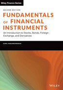
To prove this consider the following strategy. Buy the stock at the prevailing price; sell a call with an exercise price of X and a time to maturity of T − t; buy a put with the same exercise price and expiration date; and borrow the present value of the exercise price. The strategy and its implications in terms of current and future cash flows is depicted in Table 7.1.
Let us analyze the entries in Table 7.1. The first column represents the transactions that form components of the overall strategy. The second column depicts the cash flow corresponding to each transaction. If an asset results in a cash inflow, the initial cash flow will be shown with a positive sign, whereas if it results in a cash outflow, the initial cash flow will have a negative sign. When an asset is bought there will be an outflow, whereas when an asset is sold there will be a cash inflow. Similarly, when funds are borrowed there will be an inflow, whereas when funds are lent there will be a cash outflow.
TABLE 7.1 Illustration of Put-Call Parity: Strategy 1
| Terminal Cash Flow | |||
|---|---|---|---|
| Action | Initial Cash Flow | If ST > X | If ST < X |
| Buy the Stock | –St | ST | ST |
| Sell the Call | CE,t | –(ST – X) | 0 |
| Buy the Put | –PE,t | 0 | X − ST |
| Borrow the P.V. of X |  | –X | –X |
| Total | 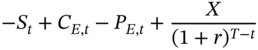 | 0 | 0 |
The third and fourth columns depict the cash flows at the time of expiration of the option. The variable of relevance is the terminal stock price and its level with respect to the exercise price of the options. There are two possibilities, that is, the stock price may be more than the exercise price or it can be less than it. Irrespective of the stock price, the stock can be sold at the prevailing stock price. If the call is in the money, it will be exercised by the counterparty, whose cash flow will be ST − X, so the arbitrageur's cash flow will be –(ST − X). If the put is in the money, it will be exercised by the arbitrageur, who will receive X − ST. Finally, because the present value of X has been borrowed at the outset, there will be an outflow of $X at the time of the expiration of the option, because the borrowed amount has to be returned with interest.
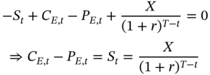
As can be seen from Table 7.1, the net cash flow at the point of expiration of the options is zero, irrespective of whether the terminal stock price is above the exercise price or below it. Thus, to rule out arbitrage we require that the initial cash flow be nonpositive, because if we have a cash inflow at the outset, followed by no further outflows, then it would clearly be a case of arbitrage. Therefore, to rule out arbitrage, we require that:
If, however,  , then we can make an arbitrage profit by simply reversing the above strategy, as demonstrated in Table 7.2.
If as assumed earlier that 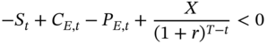 , then the initial cash flow in this case will be positive, whereas the terminal cash flows irrespective of the value of the stock price will continue to be zero.
TABLE 7.2 Illustration of Put-Call Parity: Strategy 2
| Terminal Cash Flow | |||
|---|---|---|---|
| Action | Initial Cash Flow | If ST > X | If ST < X |
| Short Sell the Stock | St | – ST | – ST |
| Buy the Call | –CE,t | (ST − X) | 0 |
| Sell the Put | PE,t | 0 | –(X − ST) |
| Lend the P.V. of X |  | X | X |
| Total | 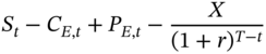 | 0 | 0 |
Hence to ensure the total absence of arbitrage, we require that:
This relationship is referred to as put-call parity. The expression that we have derived is valid only for European options on a non-dividend-paying stock. We will subsequently derive the equivalent expression for European options on a dividend-paying stock.
We will now consider the arbitrage strategies that can yield a profit if this relationship were to be violated. First assume that C − P > S − PV(X). There are three possibilities: the call may be overpriced, and/or the put may be underpriced, and/or the stock may be underpriced. Anything that is perceived as being overpriced must be sold, while an asset that is thought to be underpriced must be bought. Thus, to exploit such a situation, the call must be sold, and the stock and put must be bought. The acquisition of the stock can be funded by using borrowed money.
On the other hand, what if C − P < S − PV(X)? The possibilities are that the call is underpriced, and/or the put is overpriced, and/or the stock is overpriced. Thus, to exploit this situation, the stock must be sold short, the put must be sold, while the call must be bought.
IMPLICATIONS FOR THE TIME VALUE
If the call is in the money, the time value is P + [X − PV(X)], which cannot be negative. If the call is at or out of the money, the entire premium consists of time value. Because the premium cannot be negative, nor can the time value. Thus, European calls on a non-dividend-paying stock will always have a positive time value, except at expiration when they will have a zero time value.
Now let us consider puts.
If the put is at or out of the money, the entire premium consists of time value, and consequently the time value cannot be negative. If the put is in the money, the time value is C + {PV(X) − X]. C cannot be negative; however, PV(X) − X is negative. Hence the time value can be negative if the call premium is very low, which would mean that the call is substantially out of the money. If so, a put with the same exercise price will be substantially in the money. Thus, deep in-the-money European puts on a non-dividend-paying stock may have a negative time value.
Rationale: For a given intrinsic value, the longer the wait until exercise, the greater is the interest earned on the exercise price for a European call holder. Thus, the longer the term to maturity of the option, the greater is the premium.
In the case of puts for a given intrinsic value, however, the longer the wait to receive the exercise price, the greater is the interest lost from the inability to invest. This could lead a situation where the time value is negative. For instance, if the stock price is close to zero, the holder would love to exercise immediately; however, the European nature of the option prevents him from doing so. The longer the wait under these circumstances, the greater is the loss for the put holder. Thus, deep in-the-money European put options on a non-dividend-paying stock may have a negative time value.
PUT-CALL PARITY WITH DIVIDENDS
Let us now consider European call and put options on a stock with an exercise price of $X and T − t periods to maturity. Assume that the stock will pay a dividend of $D at a time t*, where t < t* < T. The put-call parity relationship for such options may be stated as:
To prove this, consider the strategy depicted in Table 7.3.
It is very similar to the strategy used earlier to demonstrate the put-call parity relationship for a non-dividend-paying stock. The difference is that the stock we have bought is scheduled to pay a known dividend at time t*. To make the net cash flow at this point in time equal to zero, we assume that the trader borrows the present value of this dividend at the outset. Because the dividend is scheduled to be paid at t*, the present value is  .
.
As can be seen from Table 7.3, the cash flows at all subsequent points in time are guaranteed to be zero. Hence, to rule out arbitrage we require that the initial cash flow be nonpositive. If the initial cash flow were to be negative, however, we can reverse the above strategy and make arbitrage profits. Consequently, to rule out all forms of arbitrage, we require that:
This can be extended to the case of multiple dividends.
TABLE 7.3 Illustration of Put-call Parity for a Dividend-paying Stock
| Actions | Initial Cash Flow | Intermediate Cash flow | Terminal Cash flow | |
|---|---|---|---|---|
| If ST > X | If ST < X | |||
| Buy the Stock | –St | D | ST | ST |
| Sell the Call | CE,t | –(ST − X) | 0 | |
| Buy the Put | –PE,t | 0 | X − ST | |
| Borrow the P.V. of D |  | −D | ||
| Borrow the P.V. of X |  | –X | –X | |
| Total | 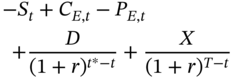 | 0 | 0 | 0 |
IMPLICATIONS FOR THE TIME VALUE
If the option is at or out of the money, the time value cannot be negative. For in-the-money calls, however, the time value is ![]() . The put premium cannot be negative and neither can the difference between the exercise price and its present value. But the third term, –PV(D), will be less than zero. Hence if P is very low and D is high, the call option may have a negative time value. If P is very low, the put will be substantially out of the money, which would mean that the call will be substantially in the money. Thus, deep in-the-money European calls on a dividend-paying stock may have a negative time value. There are conflicting forces at work here. The longer the exercise is delayed, the greater the income earned from investing the exercise price. If there is a large dividend before exercise, however, the holder may like to exercise and receive the dividend, which can then be reinvested. The longer the term to maturity of the option, the greater is the lost interest due to the inability to reinvest the dividend. The larger the magnitude of the dividend, the more is the lost interest. Thus, European in-the-money calls on a dividend-paying stock may have a negative time value.
. The put premium cannot be negative and neither can the difference between the exercise price and its present value. But the third term, –PV(D), will be less than zero. Hence if P is very low and D is high, the call option may have a negative time value. If P is very low, the put will be substantially out of the money, which would mean that the call will be substantially in the money. Thus, deep in-the-money European calls on a dividend-paying stock may have a negative time value. There are conflicting forces at work here. The longer the exercise is delayed, the greater the income earned from investing the exercise price. If there is a large dividend before exercise, however, the holder may like to exercise and receive the dividend, which can then be reinvested. The longer the term to maturity of the option, the greater is the lost interest due to the inability to reinvest the dividend. The larger the magnitude of the dividend, the more is the lost interest. Thus, European in-the-money calls on a dividend-paying stock may have a negative time value.
Now consider puts. ![]() .
.
Once again, at-the-money and out-of-the-money puts cannot have a negative time value. For an in-the-money put, the time value is ![]() . The first two terms are nonnegative while the third is negative. If C is very low, which means that the put is substantially in the money, the time value, as in the case of puts on a non-dividend-paying stock, may be negative. For a given set of a parameters, the lower the magnitude of the dividend, the greater the likelihood of the time value being negative.
. The first two terms are nonnegative while the third is negative. If C is very low, which means that the put is substantially in the money, the time value, as in the case of puts on a non-dividend-paying stock, may be negative. For a given set of a parameters, the lower the magnitude of the dividend, the greater the likelihood of the time value being negative.
A VERY IMPORTANT PROPERTY FOR AMERICAN CALLS
We will now demonstrate that an American call on a non-dividend-paying stock will never be exercised early, that is, prior to expiration. In other words, an American call on a non-dividend-paying stock is exactly equivalent to a European call on the same stock.
Consider the strategy outlined in Table 7.4.
Assume that the initial cash flow is positive. That is:
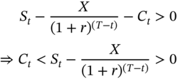
In the table, the initial cash flow has been assumed to be positive. The cash flows at the time of expiration of the option will be nonnegative, as can be seen, whether the option is in the money or out of it. The cash flow at the intermediate point in time t*, however, looks to be negative. Let us analyze this.
First, why are we concerned with the situation at a time prior to expiration? The reason is that this proof is intended to be common for both European and American options. And whenever we seek to present a result for American options, we need to factor in the consequences of early exercise. In this strategy arbitrageurs have bought the call. If they were to prematurely exercise it, it will lead to an overall cash outflow. Because the option is in their control, however, they will obviously never exercise it early in such circumstances. Thus, we do not have to consider the possibility of a negative cash flow prior to expiration. Hence irrespective of the subsequent movements in the stock price, this strategy will give rise to nonnegative cash flows. So, to rule out arbitrage, the initial cash flow must be nonpositive. Thus:
TABLE 7.4 Lower Bound for Call Options
| Intermediate Cash flow | Terminal Cash flow | |||
|---|---|---|---|---|
| Actions | Initial Cash Flow | If St* > X | If ST > X | If ST < X |
| Short Sell the Stock | St | –St* | –ST | –ST |
| Buy the Call | –Ct | (St* − X) | (ST − X) | 0 |
| Lend the P.V. of X |  |  | X | X |
| Total |  |  | 0 | X − ST > 0 |
But what if 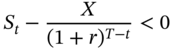 ? Then we can state that Ct > 0, for we know that an option cannot have a negative premium. Thus, combining the two conditions we can state that:
We know that an American option must trade at least for its intrinsic value. That is: Ct > Max[0, St − X]. But if  , then this condition will be automatically satisfied. Thus, the condition that we have just derived gives us a tighter lower bound for the premium of an option prior to expiration. Based on this result, we can draw some important conclusions about an American call on a non-dividend-paying stock.
- An in-the-money American call will always have a positive time value except at expiration. We know that the time value of all options must be zero at expiration. From our result, however, if we assume that St > X, prior to expiration, then:

- Obviously, an American call on a non-dividend-paying stock will never be exercised early. If holders were to exercise such an option when it is in the money, they will get the intrinsic value of the option. If they were to offset their long position by taking a counterposition, however, they will get the premium, which, as we have just demonstrated, will be greater than the intrinsic value. Thus, traders who desire to get out of a long call position would rather offset than exercise prior to maturity.
- An American call on a non-dividend-paying stock must have the same premium as a European call on the same asset, with the same exercise price and expiration date. Why is an American call generally priced higher than a European call on the same asset, and with the same features? It is because the American call gives the trader the flexibility to exercise early. If, however, an option is never going to be exercised prior to maturity, then the early exercise feature will have no value, and no rational investor will pay for it. Thus, an American call on a non-dividend-paying stock must sell for the same premium as an otherwise similar European call on the same stock.
EARLY EXERCISE OF OPTIONS: AN ANALYSIS
Consider the position of investors who own a call option on a stock and have cash equal to the exercise price of the option. If they were to exercise at time t, they would get one share of stock. If the stock price were to remain constant, which would be tantamount to assuming a constant intrinsic value, the longer the wait, the greater the interest earned on the exercise price. Thus, irrespective of the intrinsic value, holders would like to wait as long as they can, which means they will wait until expiration.
Thus, under no circumstances is it beneficial to exercise an American call on a non-dividend-paying stock prior to expiration. Hence, a trader who acquires such an option will either offset it before expiration or hold it to maturity and exercise it if it is in the money.
American puts may, however, be exercised prior to expiration. Assume that a put is substantially in the money and that the market is convinced that it will finish in the money. Holders will rather exercise than wait, for if they were to exercise, they would get the exercise price, which can be immediately invested to earn the riskless rate. Waiting is suboptimal for it will delay the cash inflow and amount to a loss of interest income. In such a situation, offsetting will not be beneficial because no potential counterparty will be willing to pay a positive time value for the option.
PROFIT PROFILES
We will now depict the profit diagrams for the four basic option positions, that is:
- Long call
- Short call
- Long put
- Short put
The payoff from a long call is Max[0, ST − X], while the profit is Max[0, ST − X] − Ct. Consider a stock currently trading at $100. Call and put options with an exercise price of $100 are currently trading at $9.50 and $5.60 respectively. The payoffs and profits for the options for various values of the terminal stock price are given in Table 7.5.
The profit diagrams are as depicted in Figures 7.1 and 7.2.
The payoffs and profits for short call and put positions are as shown in Table 7.6.
TABLE 7.5 Payoffs and Profits for Long Call and Put Positions
| Terminal Stock Price | Payoff for Call | Profit for Call | Payoff for Put | Profit for Put |
|---|---|---|---|---|
| 50 | 0 | –950 | 5,000 | 4,440 |
| 60 | 0 | –950 | 4,000 | 3,440 |
| 70 | 0 | –950 | 3,000 | 2,440 |
| 80 | 0 | –950 | 2,000 | 1,440 |
| 90 | 0 | –950 | 1,000 | 440 |
| 94.40 | 0 | –950 | 560 | 0 |
| 100 | 0 | –950 | 0 | –560 |
| 109.50 | 950 | 0 | 0 | –560 |
| 110 | 1,000 | 50 | 0 | –560 |
| 120 | 2,000 | 1,050 | 0 | –560 |
| 130 | 3,000 | 2,050 | 0 | –560 |
| 140 | 4,000 | 3,050 | 0 | –560 |
| 150 | 5,000 | 4,050 | 0 | –560 |

FIGURE 7.1 Profit Diagram for a Long Call Position

FIGURE 7.2 Profit Diagram for a Long Put Position
TABLE 7.6 Payoffs and Profits for Short Call and Put Positions
| Terminal Stock Price | Payoff for Call | Profit for Call | Payoff for Put | Profit for Put |
|---|---|---|---|---|
| 50 | 0 | 950 | –5,000 | –4,440 |
| 60 | 0 | 950 | –4,000 | –3,440 |
| 70 | 0 | 950 | –3,000 | –2,440 |
| 80 | 0 | 950 | –2,000 | –1,440 |
| 90 | 0 | 950 | –1,000 | –440 |
| 94.40 | 0 | 950 | –560 | 0 |
| 100 | 0 | 950 | 0 | 560 |
| 109.50 | –950 | 0 | 0 | 560 |
| 110 | –1,000 | –50 | 0 | 560 |
| 120 | –2,000 | –1,050 | 0 | 560 |
| 130 | –3,000 | –2,050 | 0 | 560 |
| 140 | –4,000 | –3,050 | 0 | 560 |
| 150 | –5,000 | –4,050 | 0 | 560 |

FIGURE 7.3 Profit Diagram for a Short Call Position
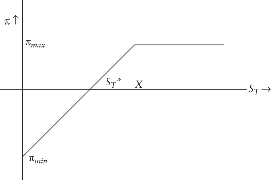
FIGURE 7.4 Profit Diagram for a Short Put Position
SPECULATION WITH OPTIONS
Traders can use options contracts for speculation. Bulls can take a long position in call options or short positions in put options. In either case, they stand to make a profit if they are right, and the market does rise. Figure 7.3 depicts the profit profile for a short call position while Figure 7.4 depicts the equivalent profile for a short put position.
In the case of speculators who take short positions in options, the losses can be significant, as the following example illustrates.
Bears can also use options to speculate. In their case, they will have to use a long position in put options or a short position in call options.
HEDGING WITH OPTIONS
Call and put options can be used to hedge the risk associated with spot positions. We will study two hedging strategies, using calls to hedge a short spot position, and using puts to hedge a long spot position.
Using Call Options to Protect a Short Position
Call options can be used to hedge the risk associated with a short spot position. To implement the strategy, the trader needs to acquire a call option for every share that is sold short. The profit from the short spot position is St − ST. The profit from the long call is Max[0, ST − X] − Ct. Thus, the total profit is equal to:
If the option were to expire in the money, the call will be exercised. The total profit in this case will be: St − X − Ct. This represents the minimum profit from the position. If the option were to expire out of the money, however, the call will expire worthless, and the profit will be: St − ST − Ct. The break-even stock price is given by:
The maximum profit will arise if the stock price were to attain a value of zero, and will be equal to St − Ct. Thus, the hedged position puts a cap on the loss in the event of an adverse market movement, but enables the trader to benefit from a positive market movement.
Thus, the maximum loss is capped at $1,090. The break-even point is 89.10, which is 100 − 10.90 = St − Ct. The position leaves the trader with the opportunity to take advantage of price movements on the downside.
Using Put Options to Protect a Long Spot Position
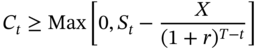
Similarly, put options can be used to protect a long spot position from price risk. In this case, hedgers have to buy one put option for every stock that they acquire. The profit from the long stock position is: ST − St. The profit from the long put position is: Max[0, X − ST] − Pt. Thus the profit from the overall position is: ![]() . If the terminal stock price were to be below the exercise price, the puts will be exercised, and the overall profit will be X − St − Pt. This represents the maximum loss from the position. If the option were to end up out of the money, the profit will be ST − St − Pt. The break-even point is given by ST* = St + Pt. There is obviously no upper limit on the profit. Once again, the hedge puts a cap on the loss, while permitting traders to take advantage of favorable market movements.
. If the terminal stock price were to be below the exercise price, the puts will be exercised, and the overall profit will be X − St − Pt. This represents the maximum loss from the position. If the option were to end up out of the money, the profit will be ST − St − Pt. The break-even point is given by ST* = St + Pt. There is obviously no upper limit on the profit. Once again, the hedge puts a cap on the loss, while permitting traders to take advantage of favorable market movements.
Thus, the maximum loss is capped at $600. The break-even point is 106, which is 100 + 6 = St + Pt. The position leaves the trader with the opportunity to take advantage of price movements on the upside.
VALUATION
Options, unlike futures contracts, cannot be priced by ruling out simple cash-and-carry and reverse cash-and-carry arbitrage strategies. The value of an option depends on the probability that it will finish in the money, and on the payoff if it does so. Consequently, to price an option, we need to make an assumption about the process for the evolution of the price of the underlying asset over time. The pricing formula obtained would depend on the price process that is postulated. In some cases, we will arrive at precise mathematical formulae, or what we term as closed-form solutions, while in other cases the best we can do is to come up with a numerical approximation.
The price of an option, irrespective of the price process assumed, is a function of the following variables.
The Price of the Underlying Asset: Because the option is based on the underlying asset, its price will depend on the price of the underlying asset. Keeping all the other variables constant, the higher the price of the underlying asset, the higher will be the value of a call option, and the lower will be the value of a put option.
The Exercise Price: The partial derivative of the option premium with respect to the exercise price will be negative for call options and positive for put options, as is to be expected. That is, the higher the exercise price, ceteris paribus, the lower will be the call premium and the higher will be the put premium.
Dividends: When a stock goes ex-dividend, the share price will decline immediately. Because the call premium is positively related to the stock price, the larger the dividend, the lower will be the call premium. Similar logic tells us that the larger the dividend, the higher will be the put premium. It must be clarified that the only dividends of consequence are those that are scheduled to be paid during the life of the options contract.
Volatility: In finance we typically assume that investors are risk averse. That is, for a given level of expected returns, the greater the risk as measured by the standard deviation or variance, the lower will be the utility. Options, however, are different. Both calls and puts, being contingent contracts, protect the holders from price movements on one side while permitting them to take full advantage of movements on the other side. This is because the worst that can happen to call holders is that they will lose the option premium, no matter how low the stock price may go. Similarly, irrespective of the increase in the stock price, a put holder can never lose more than the premium. Thus, the higher the volatility the greater will be the values of both call and put options.
Time to Maturity: Most options are what are termed as wasting assets, that is, keeping all the other variables constant, their value steadily erodes over time. Most options, with the exception of certain European options, have a positive time value prior to expiration. At the point of expiration, as we have seen earlier, all options must have a zero time value to rule out arbitrage. Thus, most options will experience a steady decline of value over time, if the other variables that influence the price remain constant.
The Riskless Interest Rate: Take the case of an investor who has adequate funds to acquire a stock at its prevailing price. One alternative would be to buy a call option and invest the balance at the riskless rate. The higher the interest rate, the more attractive will be the second course of action. Consequently, the higher the interest rate, the greater will be the demand for the call, and hence the greater will be the premium of a call option.
To draw a conclusion for put options, let us look at the issue from the perspective of an investor who owns the underlying asset and is contemplating its sale. One alternative is to buy a put option and thereby lock in a minimum price for the asset. The higher the prevailing rate of interest, the more enticing will be the prospect of an immediate sale followed by reinvestment of the sale proceeds. Consequently, the higher the interest rate, the lower will be the demand for put options, and the lower will be the value of a put option.
THE BINOMIAL OPTION PRICING MODEL
This model assumes that given a state of nature characterized by a price St, at the end of the next period the asset price may either go up to uSt or go down to dSt, where u is obviously greater than 1.0, while d is less than 1.0. Because the asset can only take on one of two possible values at the end of every time period, the model is termed as the binomial model.
We will first consider the one-period case; that is, we will assume that we are at time (T − 1), where T is the scheduled expiration date of the option. The evolution of the asset price may be depicted as shown in Figure 7.5.
Our objective is to find the option premium at (T − 1). We have to commence our computation from the point of expiration, because that is the instant at which we know what the payoff from the contract will be. Thus, in the binomial model, we always start by considering the cash flows from the option at the point of expiration.
If the upstate is reached, the payoff from a call option will be Cu = Max[0, uSt − X], whereas if the downstate is reached, it will be Cd = Max[0, dSt − X].
Consider a portfolio consisting of α shares of stock and a short position in a call option. α is termed as the hedge ratio. The current value of the portfolio is αSt − Ct, where Ct is the unknown call premium that we are seeking to derive. Next period, in the upstate the portfolio will be worth αuSt − Cu, while in the downstate it will be worth αdSt − Cd. We will choose the hedge ratio in such a way that the payoff in the upstate is the same as that in the downstate. That is:

This portfolio by construction is riskless because the payoff is identical in both states of nature. To rule out the prospect of arbitrage, it must therefore earn the riskless rate of return. That is:

FIGURE 7.5 Stock Price Tree for the One-period Case
where r is one plus the riskless rate per period.1
Therefore

p and (1 − p) are referred to as risk-neutral probabilities. Thus, the value of the option as per this model is a probability-weighted average of the option values in the up and down states.
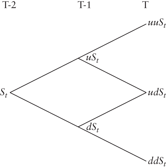
FIGURE 7.6 Stock Price Tree for the Two-period Case
THE TWO-PERIOD MODEL
In the preceding exposition we assumed that the stock price will move just once prior to the expiration of the option. In general, the asset price will move many times before the expiration of the options contract. The arguments used for the one-period case can be extended to value an option in a multi-period framework.
Let us assume that the current stock price is St, and that there are two periods left until the expiration date of the option. The evolution of the stock price is depicted in Figure 7.6.
As we did in the one-period case, we know the payoffs at expiration. Let us step back one period from T to T − 1, to compute the option price. As this is a one-period problem, we can state that

We know the values of Cuu, Cud, and Cdd, because they represent the payoffs at the three nodes corresponding to the expiration date of the option. Once we have computed the values of Cu and Cd, we can once again invoke the one-period model to evaluate Ct, which is the value of the option at T − 2. This is the basis on which we will solve the multi-period option pricing problem. That is, we start at expiration, and repeatedly invoke the one-period logic to compute the value of the option at a node corresponding to a previous point in time. We will now present the solution for the two-period problem using the data in Example 7.24.
VALUATION OF EUROPEAN PUT OPTIONS
Let us consider the one-period case first. Define Pu = Max[0, X −uSt] and Pd = Max[0, X − dSt]. The option premium at a prior point in time may be computed as a probability-weighted average of the payoffs at expiration, where the risk-neutral probabilities have the same definition as before. When we extend the theory to the multi-period case, we once again start at the expiration date of the option and work backwards, one step at a time, by repeatedly invoking the one-period model. Example 7.25 demonstrates the valuation process for a two-period put option.
VALUING AMERICAN OPTIONS
The binomial model can be easily extended to value American options. At each node we have to compare the model value, obtained by working backwards from the following point in time, with the intrinsic value of the option. If the intrinsic value is greater than the model value, we use it to compute the option premium for subsequent calculations. The rationale is that if the model value is lower than the intrinsic value at a particular node, then the holders will choose to exercise it early. If they do not wish to hold the option, then obviously early exercise will occur. This is because although offsetting is an alternative for such investors, it will not be optimal because potential buyers will not pay more than the model value for the option, since buyers can always replicate the option at the model value. Thus, early exercise is superior to taking a counterposition under such circumstances. Even if the holders were to desire to continue holding the option, it would be more profitable to exercise it, realize the intrinsic value, and replicate it at a cost lower than the intrinsic value.
We demonstrate the valuation of an American put option in Example 7.26.2
IMPLEMENTING THE BINOMIAL MODEL IN PRACTICE
While illustrating the binomial model we have arbitrarily assumed values for u, d, and consequently p. In practice, these parameters are chosen such that the moments of the discrete-time asset price process correspond to the moments of the lognormal distribution. The significance of the lognormal distribution is that it is the price process assumed by Black and Scholes in order to derive their option pricing model.
If σ is the standard deviation of the rate of return on the underlying asset, i is the annual riskless rate, and Δt is the length of a period in the binomial process being modeled, as measured in years, the normal practice is to set
THE BLACK-SCHOLES MODEL
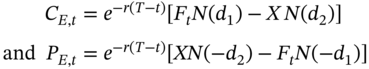
Black and Scholes derived closed-form solutions for the values of European call and put options on non-dividend-paying stocks by assuming that stock prices follow a lognormal process. The Black-Scholes formula for a European call option may be stated as follows.
The formula for European put options is
In these formulae

and ![]() .
.
N(X) is the cumulative probability distribution function for a standard normal variable.
PUT-CALL PARITY
Put-call parity is a relationship that must be satisfied if arbitrage is to be ruled out. Consequently, it is independent of the model that is used to price the options and we would therefore expect the Black-Scholes model to satisfy it. We will now demonstrate that the formula indeed satisfies the put-call parity condition.
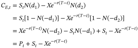
INTERPRETATION OF THE BLACK-SCHOLES FORMULA
The option price as per the formula is independent of the risk preferences of traders. If the attitude toward risk is indeed irrelevant, the simplest approach to valuation would entail the assumption that all investors are risk neutral. A risk-neutral investor would value any asset as the present value of the expected payoff, where the discount rate used will be the riskless rate.
From the Black-Scholes formula for call options:
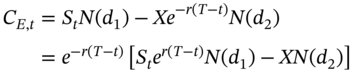
Thus ![]() is the expected payoff from the option at the time of expiration as perceived by a world of risk-neutral investors.
is the expected payoff from the option at the time of expiration as perceived by a world of risk-neutral investors.
![]() is the expected value of a variable, once again in a risk-neutral world, that has a value equal to ST if the option is exercised and a value of zero otherwise. XN(d2) is the expected outflow on account of the exercise price. Because the exercise price has to be paid only if the option is exercised, N(d2) is the probability that the option will be exercised. In other words, N(d2) is the probability that the option will end up in the money, that is, the odds that ST > X.
is the expected value of a variable, once again in a risk-neutral world, that has a value equal to ST if the option is exercised and a value of zero otherwise. XN(d2) is the expected outflow on account of the exercise price. Because the exercise price has to be paid only if the option is exercised, N(d2) is the probability that the option will be exercised. In other words, N(d2) is the probability that the option will end up in the money, that is, the odds that ST > X.
For a put option

Using similar logic ![]() is the expected value of a variable that will be equal to ST if ST < X and will be zero otherwise. Obviously, N(–d2) is the probability that the put will end up in the money and will consequently be exercised.
is the expected value of a variable that will be equal to ST if ST < X and will be zero otherwise. Obviously, N(–d2) is the probability that the put will end up in the money and will consequently be exercised.
THE GREEKS
The option price is a function of many different variables that we have discussed earlier. The rate of change of the option premium with respect to these variables is denoted by Greek symbols. Hence this part of option valuation theory is referred to as The Greeks.
The partial derivative of the option price with respect to the price of the underlying asset is termed as delta. For a call option, delta will always be between zero and one. For deep out-of-the-money options, delta will be close to zero, while for deep in-the-money options it will be close to one. Delta itself is a function of several variables, including the price of the underlying asset. Consequently, delta will change as the asset price changes, and a given value of delta is valid only for an infinitesimal change in the price of the asset.
Even if the asset price were to remain constant, delta will change with the passage of time. As the time to expiration nears, delta will tend toward one if the call is in the money and will tend toward zero if the option is out of the money. Put options have a delta between zero and minus one.
The rate of change of delta with respect to the price of the underlying asset is termed as the gamma of the option. Gamma is positive for both calls and puts and tends to be at its highest when the option is close to the money.
The rate of change of the option premium with respect to the volatility of the rate of return is termed as vega. Because volatility will be perceived positively by both call and put holders, vega will be positive for both types of options.
The time decay of the option is denoted by theta. That is, theta is the negative of the partial derivative of the option premium with respect to the time remaining until maturity. Most options, with the exception of certain European options, are wasting assets; that is, their time values will steadily approach zero as expiration approaches. Because the time value at expiration must be zero for all options, theta will be negative for most options. Certain European options may have a negative time value prior to expiration. In such cases, theta will be positive because the time value must increase so as to attain a value of zero at expiration.
The rate of change of the option premium with respect to the riskless rate of interest is termed as rho. As discussed earlier, rho will be positive for call options and negative for put options.
From the put-call parity relationship for European options on a non-dividend-paying stock:
Thus, we can make the following assertions:
- The delta of a call will be equal to one plus the delta of a put.
- The gamma of call and put options will be equal.
- The vega of both call and put options will be equal.
If options were to be priced as per the Black-Scholes model, the expressions for the Greeks will be as follows.
- The call delta will be N(d1) and the put delta will be –N(–d1)
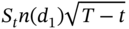
- The gamma for both calls and puts will be

- Vega for both calls and puts will be
- The theta for a call will be

The theta for a put will be
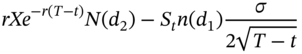
- The rho for a call will be
 while that for a put will be
  .
.
OPTION STRATEGIES
Options contracts can be used to implement various trading strategies. We will discuss two types of strategies, spreads and combinations. We will look at three categories of spreads, namely bull spreads, bear spreads, and butterfly spreads, and two types of combinations, straddles and strangles.
Bull Spreads
Bull spreads lead to a profit for the trader if the stock price were to rise; hence the name. It can be implemented using both call and put options. A bull spread, whether set up with calls or puts, sets a cap on both the loss and the profit from the strategy.
Let us first analyze a spread using calls. We will denote the two exercise prices by X1 and X2 where X1 < X2. The strategy requires the trader to buy an option with a lower exercise price and sell an option with a higher exercise price. Because the lower the exercise price, the higher will be the option premium, this strategy involves a net investment. The payoff from the strategy at expiration for various values of the terminal stock price is depicted in Table 7.9.
The minimum payoff is zero while the maximum payoff is X2 − X1. If we denote the initial investment by ΔC, then the maximum loss is –ΔC, while the maximum profit is X2 − X1 − ΔC. The break-even stock price is X1 + ΔC.
TABLE 7.9 Payoffs from a Bull Spread with Calls
| Terminal Price Range | Payoff from Long Call | Payoff from Short Call | Total Payoff |
|---|---|---|---|
| ST < X1 | 0 | 0 | 0 |
| X1 < ST < X2 | ST − X1 | 0 | ST − X1 |
| ST > X2 | ST − X1 | – (ST − X2) | X2 − X1 |

FIGURE 7.8 Profit Profile: Bull Spread
The profit diagram may be depicted as shown in Figure 7.8.
A bull spread can also be created using puts. The trader has to buy the put with the lower exercise price and sell the put with the higher exercise price. Because the put premium increases with the exercise price, the inflow from the option that is sold will be higher than the outflow on account of the option that is bought. Consequently, a bull spread with puts will lead to a cash inflow at inception. The payoff from the strategy at expiration for various values of the terminal stock price is depicted in Table 7.10.
The minimum payoff is X1 − X2 and the maximum payoff is zero. If we denote the initial inflow as ΔP, then the maximum loss is X1 − X2 + ΔP and the maximum profit is ΔP. The break-even stock price is X2 − ΔP.
TABLE 7.10 Payoffs from a Bull Spread with Puts
| Terminal Price Range | Payoff from Long Put | Payoff from Short Put | Total Payoff |
|---|---|---|---|
| ST < X1 | X1 − ST | − (X2 − ST) | X1 − X2 |
| X1 < ST < X2 | 0 | − (X2 − ST) | ST − X2 |
| ST > X2 | 0 | 0 | 0 |
Bear Spreads
Bear spreads lead to a profit for the trader if the stock price were to decline; hence the name. It can be implemented using both call and put options. A bear spread, whether set up with calls or with puts, sets a cap on both the loss and the profit from the strategy.
Let us first analyze a spread using calls. We will denote the two exercise prices by X1 and X2 where X1 < X2. The strategy requires the trader to sell an option with a lower exercise price and buy an option with a higher exercise price. Because the lower the exercise price, the higher will be the option premium, this strategy involves a cash inflow at inception. The payoff from the strategy at expiration for various values of the terminal stock price is depicted in Table 7.12.
TABLE 7.12 Payoffs from a Bear Spread with Calls
| Terminal Price Range | Payoff from Long Call | Payoff from Short Call | Total Payoff |
|---|---|---|---|
| ST < X1 | 0 | 0 | 0 |
| X1 < ST < X2 | 0 | – (ST − X1) | X1 − ST |
| ST > X2 | ST − X2 | – (ST − X1) | X1 − X2 |
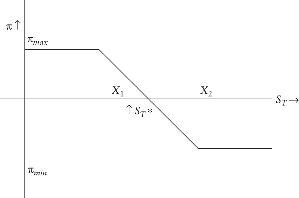
FIGURE 7.9 Profit Profile: Bear Spread
The maximum payoff is zero while the minimum payoff is X1 − X2. If we denote the initial inflow by ΔC, then the maximum profit is ΔC, while the maximum loss is X1 − X2 + ΔC. The break-even stock price is X1 + ΔC.
The profit diagram may be depicted as shown in Figure 7.9.
A bear spread can also be created using puts. The trader has to sell the put with the lower exercise price and buy the put with the higher exercise price. Because the put premium increases with the exercise price, the outflow on account of the option that is bought will be higher than the inflow on account of the option that is sold. Consequently, a bear spread with puts will lead to a cash outflow at inception. The payoff from the strategy at expiration for various values of the terminal stock price is depicted in Table 7.13.
TABLE 7.13 Payoffs from a Bear Spread with Puts
| Terminal Price Range | Payoff from Long Put | Payoff from Short Put | Total Payoff |
|---|---|---|---|
| ST < X1 | X2 − ST | − (X1 − ST) | X2 − X1 |
| X1 < ST < X2 | (X2 − ST) | 0 | X2 − ST |
| ST > X2 | 0 | 0 | 0 |
The minimum payoff is zero and the maximum payoff is X2 − X1. If we denote the initial investment as ΔP, then the maximum loss is –ΔP and the maximum profit is X2 − X1 − ΔP. The break-even stock price is X2 − ΔP.
Butterfly Spread
A butterfly spread requires options with three different exercise prices. To set up a long butterfly spread with calls, the trader will take a long position in an in-the-money call and an out-of-the-money call, and take a short position in two at-the-money calls. A butterfly spread can also be set up using put options, as we shall shortly demonstrate.
We will denote the exercise prices by X1, X2, and X3 where X1 < X2 < X3. The exercise prices are generally chosen so that the middle price is an arithmetic average of the other two prices. That is X2 = (X1 + X3)/2.
The Convexity Property
Consider three exercise prices X1, X2, and X3 such that X2 = wX1 + (1 − w)X3.
The convexity property states that the call and put premiums for the options with the corresponding exercise prices will be such that
Thus, it can be demonstrated that a butterfly spread will always require an initial investment which we will denote by ΔC. The payoffs from the strategy at expiration are depicted in Table 7.15.
The minimum payoff is zero and arises if the terminal stock price is either below the lowest of the exercise prices or above the highest. In either case the profit is –ΔC. This is the maximum potential loss from the strategy. The maximum profit is realized when ST = X2. There are two break-even prices: X1 + ΔC and X3 − ΔC.
The profit diagram is depicted in Figure 7.10.
TABLE 7.15 Payoffs from a Long Butterfly Spread
| Terminal Price Range | Payoff from Call with X = X1 | Payoff from Call with X = X3 | Payoff from Calls with X = X2 | Total Payoff |
|---|---|---|---|---|
| ST < X1 | 0 | 0 | 0 | 0 |
| X1 < ST < X2 | ST − X1 | 0 | 0 | ST − X1 |
| X2 < ST < X3 | ST − X1 | 0 | –2(ST − X2) | X3 − ST |
| ST > X3 | ST − X1 | ST − X3 | –2(ST − X2) | 0 |
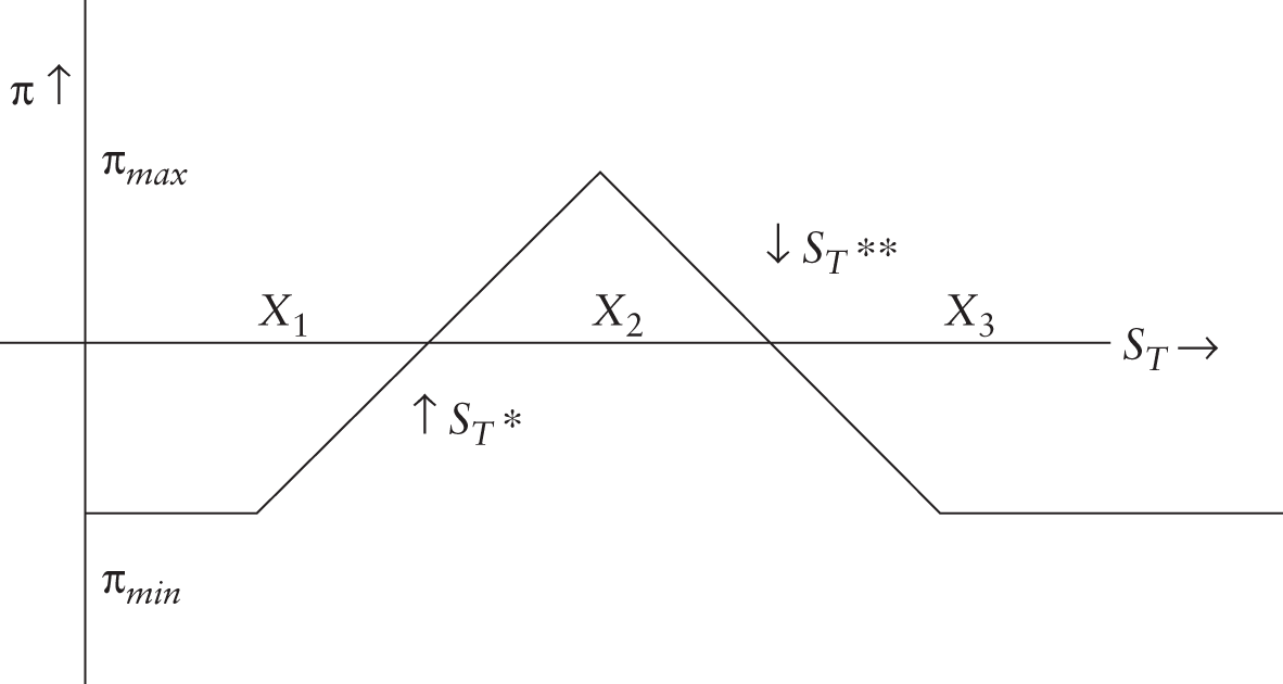
FIGURE 7.10 Profit Profile: Butterfly Spread
A butterfly spread can also be set up using put options. The strategy requires an investor to buy an in-the-money put and an out-of-the-money put, and sell two at-the-money puts, where the exercise prices are such that X1 < X2 < X3, and X2 = (X1 + X3)/2. The strategy will entail an initial investment of ΔP, which also represents the magnitude of the maximum loss. Once again, the maximum loss will be realized if the terminal stock price is below the lowest exercise price or above the highest. The two break-even prices are X1 + ΔP and X3 − ΔP.
TABLE 7.18 Payoffs from a Long Straddle
| Terminal Price Range | Payoff from Call | Payoff from Put | Total Payoff |
|---|---|---|---|
| ST < X | 0 | X − ST | X − ST |
| ST > X | ST − X | 0 | ST − X |

FIGURE 7.11 Profit Profile: Straddle
A Straddle
A long straddle requires the investor to buy a call and a put option on the same asset. Both options must have the same exercise price and expiration date. The initial investment is Ct + Pt. The call option will be in the money if the stock were to rise in value, while the put will be in the money if the stock were to decline in value. Thus, a straddle will pay off in both a bull and bear market. Consequently, it is a suitable strategy for an investor who is anticipating a large price move, but is unsure about its direction. The payoff at expiration is depicted in Table 7.18.
The maximum payoff is unlimited if ST > X, and consequently so is the maximum profit. The profit increases dollar for dollar with the stock price. In the other direction the maximum payoff is X, because the stock price cannot decline below zero. Thus, the maximum profit in this price range is X − Ct − Pt. The lowest payoff is zero, which occurs if ST = X. Hence the maximum loss is –(Ct + Pt). There are two break-even points: X − Ct − Pt and X + Ct + Pt. The profit diagram may be depicted as shown in Figure 7.11.
A Strangle
A strangle is similar to a straddle in the sense that it requires the trader to buy a call and a put on the same asset, and with the same expiration date. The difference is that the two options are chosen with different exercise prices. If we denote the exercise price of the call as X1, and that of the put as X2, there are two possibilities, that is, X1 > X2, and X1 < X2. Thus, there are two types of strangles: out-of-the-money strangles and in-the-money strangles.
Let us first consider an out-of-the-money strangle. The payoff is depicted in Table 7.20.
If ST < X2, the profit is X2 − ST − Ct − Pt. The maximum profit in this region is X2 − Ct − Pt, which is also the magnitude of the break-even stock price. If X2 < ST < X1, the payoff is zero and the loss is equal to the initial investment. This represents the maximum possible loss for this strategy. If ST > X1, the profit is ST − X1 − Ct − Pt. The maximum profit in this region is unbounded. The second break-even price is X1 + Ct + Pt. The profit diagram is depicted in Figure 7.12.
TABLE 7.20 Payoffs from an Out-of-the-money Long Strangle
| Terminal Price Range | Payoff from Call | Payoff from Put | Total Payoff |
|---|---|---|---|
| ST < X2 | 0 | X2 − ST | X2 − ST |
| X2 < ST < X1 | 0 | 0 | 0 |
| ST > X1 | ST − X1 | 0 | ST − X1 |
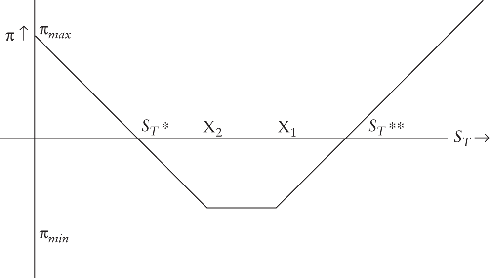
FIGURE 7.12 Profit Profile: Strangle
TABLE 7.21 Payoffs from an In-the-money Long Strangle
| Terminal Price Range | Payoff from Call | Payoff from Put | Total Payoff |
|---|---|---|---|
| ST < X1 | 0 | X2 − ST | X2 − ST |
| X1 < ST < X2 | ST − X1 | X2 − ST | X2 − X1 |
| ST > X2 | ST − X1 | 0 | ST − X1 |
Now let us consider an in-the-money strangle. The payoffs are shown in Table 7.21.
If ST < X1, the profit is X2 − ST − Pt − Ct. The maximum profit in this region is X2 − Pt − Ct, which is also the magnitude of the break-even stock price. If X1 < ST < X2, the profit is X2 − X1 − Pt − Ct. This represents the maximum loss from the strategy. Finally, if ST > X2, the profit is ST − X1 − Pt − Ct. The profit is unbounded is this region. The corresponding break-even stock price is X1 + Pt + Ct.
We will now give a numerical illustration of an out-of-the-money strangle.
FUTURES OPTIONS
A futures option is an option that is written on a futures contract. A call futures option gives holders the right to assume a long position in a futures contract if they were to exercise the option. When such a contract is exercised, a long position is established in the futures contract and the position is immediately marked to market. At this stage the holders have two options. They can either deposit the margin required to support the long futures position or they can offset the futures contract. When a call futures option is exercised by the holders, a short position in the futures contract is established for the writers of the contract, whose position will also be marked to market, and they will be confronted with the same two choices. That is, they can either deposit the margin required to maintain the futures position, or offset it.
If we denote the current futures price by Ft and the exercise price of the option by X, the contract will be exercised only if Ft > X. When the contract is marked to market there will be an inflow of Ft − X, which is nothing but the intrinsic value of the contract. What is the rationale for marking the contract to market upon exercise? The options contract gives holders the right to assume a long futures position upon exercise. When a futures position is established, it will obviously be at the prevailing futures price Ft. To ensure that the position is effectively at the exercise price, the price difference must be paid to the holders.
PUT-CALL PARITY
The put-call parity condition for European futures options is:
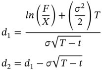
THE BLACK MODEL
The Black Model is applicable for pricing European options on futures contracts. In the case of European options scheduled to expire at the same time as the underlying futures contracts, the Black Model states that:
The variables d1 and d2 may be expressed as follows.
NOTES
- 1 The symbol r is generally used to denote the riskless rate of return. In the binomial model, however, the standard practice is to use it to denote one plus the riskless rate. In this context, r represents the periodic rate of interest, which need not necessarily be an annual rate.
- 2 An American call on a non-dividend-paying stock will obviously never be exercised early.