3

Mixing*

It will be shown that, under mild conditions, GARCH processes are geometrically ergodic and β-mixing. These properties entail the existence of laws of large numbers and of central limit theorems (see Appendix A), and thus play an important role in the statistical analysis of GARCH processes. This chapter relies on the Markov chain techniques set out, for example, by Meyn and Tweedie (1996).

3.1 Markov Chains with Continuous State Space

Recall that for a Markov chain only the most recent past is of use in obtaining the conditional distribution. More precisely, (X_t) is said to be a homogeneous Markov chain, evolving on a space E (called the state space) equipped with a σ-field ε, if for all x E, and for all ε,

(3.1)

In this equation, P^t(x, B) corresponds to the transition probability of moving from the state x to the set in t steps. The Markov property refers to the fact that P^t(x, B) does not depend on X_r, r < s. The fact that this probability does not depend on s is referred to time homogeneity. For simplicity we write P(x, B) = P¹(x, B). The function P : E × ε → [0, 1] is called a transition kernel and satisfies:

(i) ε, the function P(·, ) is measurable;

(ii) x E, the function P(x, ·) is a probability measure on (E,ε).

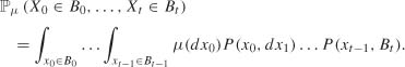
The law of the process (X_t) is characterized by an initial probability measure μ and a transition kernel P. For all integers t and all (t + l)-tuples (₀,…, _t) of elements of ε, we set

(3.2)

In what follows, (X_t) denotes a Markov chain on E = ^d and ε is the Borel σ -field.

Irreducibility and Recurrence

The Markov chain (X_t) is said to be ø-irreducible for a nontrivial (that is, not identically equal to zero) measure ø on (E,ε), if

If (X_t) is ø-irreducible, it can be shown that there exists a maximal irreducibility measure, that is, an irreducibility measure M such that all the other irreducibility measures are absolutely continuous with respect to M. If M() = 0 then the set of points from which is accessible is also of zero measure (see Meyn and Tweedie, 1996, Proposition 4.2.2). Such a measure M is not unique, but the set

does not depend on the maximal irreducibility measure M. For a particular model, finding a measure that makes the chain irreducible may be a non trivial problem (but see Exercise 3.1 for an example of a time series model for which the determination of such a measure is very simple).

A ø-irreducible chain is called recurrent if

and is called transient if

Note that can be interpreted as the average time that the chain spends in when it starts at x. It can be shown that a ø-ireducible chain (X_t) is either recurrent or transient (see Meyn and Tweedie, 1996, Theorem 8.3.4). It is said that (X_t) is positive recurrent if

If a ø-irreducible chain is not positive recurrent, it is called null recurrent. For a ø-irreducible chain, positive recurrence is equivalent to the existence of a (unique) invariant probability measure (see Meyn and Tweedie, 1996, Theorem 18.2.2), that is, a probability π such that

An important consequence of this equivalence is that, for Markov time series, the issue of finding strict stationarity conditions reduces to that of finding conditions for positive recurrence. Indeed, it can be shown (see Exercise 3.2) that for any chain (X_t) with initial measure μ,

(3.3)

For this reason, the invariant probability is also called the stationary probability.

Small Sets and Aperiodicity

For a ø-irreducible chain, there exists a class of sets enjoying properties that are similar to those of the elementary states of a finite state space Markov chain. A set C ε is called a small set¹ if there exist an integer m ≥ 1 and a nontrivial measure υ on ε such that

In the AR(1) case, for instance, it is easy to find small sets (see Exercise 3.4). For more sophisti-cated models, the definition is not sufficient and more explicit criteria are needed. For the so-called Feller chains, we will see below that it is very easy to find small sets. For a general chain, we have the following criterion (see Nummelin, 1984, Proposition 2.11): C ε⁺ is a small set if there exists ε⁺ such that, for all A, ε⁺, there exists T > 0 such that

If the chain is ø-irreducible, it can be shown that there exists a countable cover of E by small sets. Moreover, each set ε⁺ contains a small set C ε⁺. The existence of small sets allows us to define cycles for ø-irreducible Markov chains with general state space, as in the case of countable space chains. More precisely, the period is the greatest common divisor (gcd) of the set

where C ε⁺ is any small set (the gcd is independent of the choice of C). When d = 1, the chain is said to be aperiodic. Moreover, it can be shown (see Meyn and Tweedie, 1996, Theorem 5.4.4.) that there exist disjoint sets D₁,…, D_d ε such that (with the convention D_d+1 = D₁):

(i) i = l,…, d, x D_i, P(x, D_i+1) = 1;

(ii) ø(E-∪D_i) = 0.

A necessary and sufficient condition for the aperiodicity of (X_t) is that there exists A ε⁺ such that for all A, ε⁺, there exists t > 0 such that

(3.4)

(see Chan, 1990, Proposition A1.2).

Geometric Ergodicity and Mixing

In this section, we study the convergence of the probability _μ(X_t ·) to a probability π(·) independent of the initial probability μ, as t → ∞.

It is easy to see that if there exists a probability measure π such that, for an initial measure μ,

(3.5)

where _μ(X_t ) is defined in (3.2) (for (₀,…, _t) = (E,…, E, )), then the probability π is invariant (see Exercise 3.3). Note also that (3.5) holds for any measure μ if and only if

On the other hand, if the chain is irreducible, aperiodic and admits an invariant probability π, for π -almost all x E,

(3.6)

where · denotes the total variation norm² (see Meyn and Tweedie, 1996, Theorem 14.0.1). A chain (X_t) such that the convergence (3.6) holds for all x is said to be ergodic. However, this convergence is not sufficient for mixing. We will define a stronger notion of ergodicity.

The chain (X_t) is called geometrically ergodic if there exists ρ (0, 1) such that

(3.7)

Geometric ergodicity entails the so-called α- and β -mixing. The general definition of the α- and β-mixing coefficients is given in Appendix A.3.1. For a stationary Markov process, the definition of the α-mixing coefficient reduces to

where the first supremum is taken over the set of the measurable functions f and g such that | f | ≤ 1, | g | ≤ 1 (see Bradley, 1986, 2005). A general process X = (X_t) is said to be α-mixing (β-mixing) if α_X(k) (β_X(k)) converges to 0 as k → ∞. Intuitively, these mixing properties characterize the decrease in dependence when past and future become sufficiently far apart. The α-mixing is sometimes called strong mixing, but β-mixing entails strong mixing because α_X(k) ≤ β_X(k) (see Appendix A.3.1).

Davydov (1973) showed that for an ergodic Markov chain (X_t), of invariant probability measure π,

It follows that α_X(k) = O(ρ^k) if the convergence (3.7) holds. Thus

(3.8)

Two Ergodicity Criteria

For particular models, it is generally not easy to directly verify the properties of recurrence, existence of an invariant probability law, and geometric ergodicity. Fortunately, there exist simple criteria on the transition kernel.

We begin by defining the notion of Feller chain. The Markov chain (X_t) is said to be a Feller chain if, for all bounded continuous functions g defined on E, the function of x defined by E(g(X_t)|X_t−1 = x) is continuous. For instance, for an AR(1) we have, with obvious notation,

The continuity of the function x → g(θx + y) for all y, and its boundedness, ensure, by the Lebesgue dominated convergence theorem, that (X_t) is a Feller chain. For a Feller chain, the compact sets C ε⁺ are small sets (see Feigin and Tweedie, 1985).

The following theorem provides an effective way to show the geometric ergodicity (and thus the β-mixing) of numerous Markov processes.

Theorem 3.1 (Feigin and Tweedie (1985, Theorem 1)) Assume that:

(i) (X_t) is a Feller chain;

(ii) (X_t) is ø-irreducible;

(iii) there exist a compact set A E such that ø (A) > 0 and a continuous function V : E → ⁺ satisfying

(3.9)

and for δ > 0,

(3.10)

Then (X_t) is geometrically ergodic.

This theorem will be applied to GARCH processes in the next section (see also Exercise 3.5 for a bilinear example). In equation (3.10), V can be interpreted as an energy function. When the chain is outside the center A of the state space, the energy dissipates, on average. When the chain lies inside A, the energy is bounded, by the compactness of A and the continuity of V. Sometimes V is called a test function and (III) is said to be a drift criterion.

Let us explain why these assumptions imply the existence of an invariant probability measure. For simplicity, assume that the test function V takes its values in [l,+∞), which will be the case for the applications to GARCH models we will present in the next section. Denote by P the operator which, to a measurable function f in E, associates the function Pf defined by

Let P^t be the tth iteration of P, obtained by replacing P(x, dy) by P^t (x, dy) in the previous integral. By convention P⁰f = f and P⁰(x, A) = _A. Equations (3.9) and (3.10) and the boundedness of V by some M > 0 on A yield an inequality of the form

where b = M − (1 − δ)., Iterating this relation t times, we obtain, for x₀ A

(3.11)

It follows (see Exercise 3.6) that there exists a constant k > 0 such that for n large enough,

(3.12)

The sequence Q_n(x₀, ·) being a sequence of probabilities on (E, ε), it admits an accumulation point for vague convergence: there exist a measure π of mass less than 1 and a subsequence (n_k) such that for all continuous functions f with compact support,

(3.13)

In particular, if we take f = _A in this equality, we obtain π(A) ≥ k, thus π is not equal to zero. Finally, it can be shown that π is a probability and that (3.13) entails that π is an invariant probability for the chain (X_t) (see Exercise 3.7).

For some models, the drift criterion (iii) is too restrictive because it relies on transitions in only one step. The following criterion, adapted from Meyn and Tweedie (1996, Theorems 19.1.3, 6.2.9 and 6.2.5), is an interesting alternative relying on the transitions in n steps.

Theorem 3.2 (Geometric ergodicity criterion) Assume that:

(i) (X_t) is an aperiodic Feller chain;

(ii) (X_t) is ø-irreducible where the support of ø has nonempty interior;

(iii) there exist a compact C E, an integer n≥1 and a continuous function V : E → ⁺ satisfying

(3.14)

and for δ > 0 and b >0,

(3.15)

Then (X_t) is geometrically ergodic.

The compact C of condition (iii) can be replaced by a small set but the function V must be bounded on C. When (X_t) is not a Feller chain, a similar criterion exists, for which it is necessary to consider such small sets (see Meyn and Tweedie, 1996, Theorem 19.1.3).

3.2 Mixing Properties of GARCH Processes

We begin with the ARCH(l) process because this is the only case where the process (_t) is Markovian.

The ARCH(l) Case

Consider the model

(3.16)

where ω > 0, α ≥ 0 and (η_t) is a sequence of iid (0, 1) variables. The following theorem establishes the mixing property of the ARCH(l) process under the necessary and sufficient strict stationarity condition (see Theorem 2.1 and (2.10)). An extra assumption on the distribution of η_t is required, but this assumption is mild:

Assumption A The law P_η of the process (η_t) is absolutely continuous, of density f with respect to the Lebesgue measure λ on (, ()). We assume that

(3.17)

and that there exists τ > 0 such that

Note that this assumption includes, in particular, the standard case where f is positive over a neighborhood of 0, possibly over all . We then have η⁰ = 0. Equality (3.17) implies some (local) symmetry of the law of (η_t). This symmetry facilitates the proof of the following theorem, but It can be omitted (see Exercise 3.8).

Theorem 3.3 (Mixing of the ARCH(l) model) Under Assumption A and for

(3.18)

the nonanticipative strictly stationary solution of the ARCH (1) model (3.16) is geometrically ergodic, and thus geometrically β-mixing.

Proof. Let ψ(x) = (ω + αx²)^½. A process (_t) satisfying

where η_t is independent of _t-i, i > 0, is clearly a homogenous Markov chain on (, ()), with transition probabilities

We will show that the conditions of Theorem 3.1 are satisfied.

Step (i). We have

If g is continuous and bounded, the same is true for the function x → g{ψ(x)y], for all y. By the Lebesgue theorem, it follows that (_t) is a Feller chain.

Step (ii). To show the ø-irreducibility of the chain, for some measure ø, assume for the moment that η⁰ = 0 in Assumption A. Suppose, for instance, that f is positive on [0, τ). Let ø be the restriction of the Lebesgue measure to the interval . Since Ψ(x) ≥ , It can be seen that

It follows that the chain (_t) is ø-irreducible. In particular, ø = λ if η_t has a positive density over .

The proof of the irreducibility in the case η⁰>0 is more difficult. First note that

Now E log α by (3.18). Thus we have

Let τ′ (0, τ) be small enough such that

Iterating the model, we obtain that, for ⁰ = x fixed,

It follows that the function

Is a diffeomorphism between open subsets of ^t. Moreover, in view of Assumption A, the vector Y_t has a density on ^t. The same is thus true for Z_t, and It follows that, given ₀=x,

(3.19)

We now Introduce the event

(3.20)

Assumption A implies that (Ξ_t) > 0. Conditional on Ξ_t, we have

Since the bounds of the interval I_t are reached, the intermediate value theorem and (3.19) entail that, given ₀ = x, has, conditionally on Ξ_t, a positive density on I_t. It follows that

(3.21)

where J_t = {x | x² I_t}. Let

and let λ_J be the restriction of the Lebesgue measure to J. We have

The chain (_t) is thus ø-irreducible with ø = λ_J.

Step (iii). We shall use Lemma 2.2. The variable α Is almost surely positive and satisfies E(α) = α < ∞ and Elogα < 0, in view of assumption (3.18). Thus, there exists s > 0 such that

where μ_2s = E^s. The proof of Lemma 2.2 shows that we can assume s ≤ 1. Let V(x) = 1 + x^2s. Condition (3.9) is obviously satisfied for all x. Let 0 < δ < 1 − c and let the compact set

Since A is a nonempty closed interval with center 0, we have ø(A) > 0. Moreover, by the inequality (a+b)^s≤a^s+b^s for a, b ≥ 0 and s [0, 1] (see the proof of Corollary 2.3), we have, for x A,

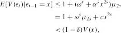
which proves (3.10). It follows that the chain (_t) is geometrically ergodic. Therefore, in view of (3.8), the chain obtained with the invariant law as Initial measure is geometrically β-mixing. The proof of the theorem is complete.        

Remark 3.1 (Case where the law of η_t does not have a density) The condition on the density of η_t is not necessary for the mixing property. Suppose, for example, that , a.s. (that is, η_t takes the values − 1 and 1, with probability ½). The strict stationarity condition reduces to α < 1 and the strictly stationary solution is a.s This solution is mixing since it is an independent white noise.

Another pathological example is obtained when η_t has a mass at 0: (η_t = 0) = θ > 0. Regardless of the value of α, the process is strictly stationary because the right-hand side of inequality (3.18) is equal to +∞. A noticeable feature of this chain is the existence of regeneration times at which the past is forgotten. Indeed, if η_t = 0 then _t = 0, , … It is easy to see that the process is then mixing, regardless of α.

The GARCH(1,1) Case

Let us consider the GARCH(1, 1) model

(3.22)

where ω>0, α ≥0, β ≥ 0 and the sequence (η_t) is as in the previous section. In this case (σ_t) is Markovian, but (_t) is not Markovian when β > 0. The following result extends Theorem 3.3.

Theorem 3.4 (Mixing of the GARCH(1,1) model) Under Assumption A and if

(3.23)

then the nonanticipative strictly stationary solution of the GARCH(1, 1) model (3.22) is such that the Markov chain (σ_t) is geometrically ergodic and the process (_t) is geometrically β-mixing.

Proof. If α = 0 the strictly stationary solution is iid, and the conclusion of the theorem follows in this case. We now assume that α > 0. We first show the conclusions of the theorem that concern the process (σ_t). A homogenous Markov chain (σ_t) is defined on (⁺,(⁺)) by setting, for t ≥ 1,

(3.24)

where a(x) = ax² + β. Its transition probabilities are given by

where _x = {η; {ω + a(η)x²}^½ }. We show the stated results by checking the conditions of Theorem 3.1.

Step (i). The arguments given in the ARCH(l) case, with

are sufficient to show that (σ_t) is a Feller chain.

Step (ii). To show the irreducibility, note that (3.23) implies

since |η_t| ≥ η⁰ a.s. and a(·) is an increasing function. Let τ′ (0,τ) be small enough such that

If σ₀ = x ⁺, we have, for t > 0,

Conditionally on Ξ_t, defined in (3.20), we have

Let

Then, given σ₀ = x,

σ_t has, conditionally on Ξ_t, a positive density on J_t

where J_t={x ⁺|x² I_xt}. Let λ_J be the restriction of the Lebesgue measure to . We have

The chain (σ_t) is thus ø-irreducible with ø = λ_J.

Step (iii). We again use Lemma 2.2. By the arguments used in the ARCH(l) case, there exists s [0, 1] such that

Define the test function by V(x) = 1 + x^2s, let 0 ≤ δ ≤ 1 − c₁ and let the compact set

We have, for x A,

which proves (3.10). Moreover (3.9) is satisfied.

To be able to apply Theorem 3.1, it remains to show that ø(A) >0 where ø is the above irreducibility measure. In view of the form of the intervals I and A, it is clear that, denoting by Å the interior of A,

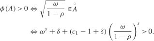
Therefore, it suffices to choose δ sufficiently close to 1 − c₁ so that the last inequality is satisfied. For such a choice of δ, the compact set A satisfies the assumptions of Theorem 3.1. Consequently, the chain (σ_t) is geometrically ergodic. Therefore the nonanticipative strictly stationary solution (σ_t), satisfying (3.24) for t , is geometrically β-mixing.

Step (iv). Finally, we show that the process (_t) inherits the mixing properties of (σ_t). Since _t = σ_tη_t, it is sufficient to show that the process Y_t = (σ_t, η_t)′ enjoys the mixing property. It is clear that (Y_t) is a Markov chain on ⁺ × equipped with the Borel σ-field. Moreover, (Y_t) is strictly stationary because, under condition (3.23), the strictly stationary solution (σ_t) is nonanticipative, thus Y_t is a function of η_t, η_t−1,… Moreover, σ_t is independent of η_t. Thus the stationary law of (Y_t) can be denoted by _Y = _{σ η} where _σ denotes the law of σ_t and _η that of η_t. Let ^t(y, ·) the transition probabilities of the chain (Y_t). We have, for y = (y₁, y₂) ⁺ × , ₁ (⁺), ₂ () and t > 0,

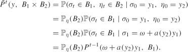
It follows, since _η is a probability, that

The right-hand side converges to 0 at exponential rate, in view of the geometric ergodicity of (σ_t). It follows that (Y_t) is geometrically ergodic and thus β-mixing. The process (_t) is also β-mixing, since _t is a measurable function of Y_t.

Theorem 3.4 is of interest because it provides a proof of strict stationarity which is completely different from that of Theorem 2.8. A slightly more restrictive assumption on the law of η_t has been required, but the result obtained in Theorem 3.4 is stronger.

The ARCH(q) Case

The approach developed in the case q = 1 does not extend trivially to the general case because (_t) and (σ_t) lose their Markov property when p>1 or q > 1. Consider the model

(3.25)

where ω > 0, α_i ≥ 0, i = 1.,…, q, and (η_t) is defined as in the previous section. We will once again use the Markov representation

(3.26)

where

Recall that γ denotes the top Lyapunov exponent of the sequence {A_t, t }.

Theorem 3.5 (Mixing of the ARCH(q) model) If η_t has a positive density on a neighborhood of 0 and γ < 0, then the nonanticipative strictly stationary solution of the ARCH(q) model (3.25) is geometrically β-mixing.

Proof. We begin by showing that the nonanticipative and strictly stationary solution () of the model (3.26) is mixing. We will use Theorem 3.2 because a one-step drift criterion is not sufficient.

Using (3.26) and the independence between η_t and the past of it can be seen that the process () is a Markov chain on (⁺)^q equipped with the Borel σ-field, with transition probabilities

The Feller property of the chain () is obtained by the arguments employed in the ARCH(l) and GARCH(1, 1) cases, relying on the independence between η_t and the past of as well as on the continuity of the function → _t + A_t.

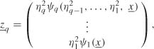
In order to establish the irreducibility, let us consider the transitions in q steps. Starting from ₀ = , after q transitions the chain reaches a state _q of the form

where the functions ψ_i- are such that ψ_i(·) ≥ ω > 0. Let τ > 0 be such that the density f of η_i be positive on (−τ, τ), and let ø be the restriction to [0, ωτ²[^q of the Lebesgue measure λ on ^q.

It follows that, for all = ₁ × … × _q ((⁺)^q), ø()>0 implies that, for all y₁,…,y_q (⁺)^qand for all i = 1,…, q,

which implies in turn that, for all (⁺)^q, P_q(,) > 0. We conclude that the chain () is ø-irreducible.

The same argument shows that

The criterion given in (3.4) can then be checked, which implies that the chain is aperiodic.

We now show that condition (iii) of Theorem 3.2 is satisfied with the test function

where · denotes the norm A = Σ |A_ij| of a matrix A = (A_ij) and s (0, 1) is such that

for some integer k₀ ≥ 1. The existence of s and k₀ is guaranteed by Lemma 2.3. Iterating (3.26), we have

The norm being multiplicative, it follows that

Thus, for all (⁺)^p+q,

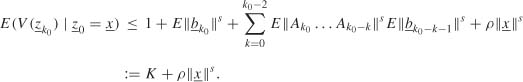
The inequality comes from the independence between A_t and _t−i for i > 0. The existence of the expectations on the right-hand side of the inequality comes from arguments used to show (2.33). Let δ > 0 such that 1. − δ > p and let C be the subset of (⁺)^p+q defined by

We have C ≠ because K > 1. − δ. Moreover, C is compact because 1 − δ − ρ > 0. Condition (3.14) is clearly satisfied, V being greater than 1. Moreover, (3.15) also holds true for n = k₀−1. We conclude that, in view of Theorem 3.2, the chain is geometrically ergodic and, when it is initialized with the stationary measure, the chain is stationary and β-mixing.

Consequently, the process (), where (_tt) is the nonanticipative strictly stationary solution of model (3.25), is βmixing, as a measurable function of This argument is not sufficient to conclude concerning (_t). For k > 0, let

where f and g are measurable functions. Note that

Similarly, we have E(Z_k |, t ) = E(Z_k|,t ≥ k) and we have independence between Y₀ and Z_k conditionally on (). Thus, we obtain

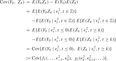
It follows, in view of the definition (A.5) of the strong mixing coefficients, that

In view of (A.6), we also have . Actually, (A.7) entails that the converse inequalities are always true, so we have and β_²(k) = β(k). The theorem is thus shown.        

3.3 Bibliographical Notes

A major reference on ergodicity and mixing of general Markov chains is Meyn and Tweedie (1996). For a less comprehensive presentation, see Chan (1990), Tj0stheim (1990) and Tweedie (1998). For survey papers on mixing conditions, see Bradley (1986, 2005). We also mention the book by Doukhan (1994) which proposes definitions and examples of other types of mixing, as well as numerous limit theorems.

For vectorial representations of the form (3.26), the Feller, aperiodicity and irreducibility properties were established by Cline and Pu (1998, Theorem 2.2), under assumptions on the error distribution and on the regularity of the transitions.

The geometric ergodicity and mixing properties of the GARCH(p, q) processes were established in the PhD thesis of Boussama (1998), using results of Mokkadem (1990) on polynomial processes. The proofs use concepts of algebraic geometry to determine a subspace of the states on which the chain is irreducible. For the GARCH(1, 1) and ARCH(q) models we did not need such sophisticated notions. The proofs given here are close to those given in Francq and Zakoïan (2006a), which considers more general GARCH(1, 1) models. Mixing properties were obtained by Carrasco and Chen (2002) for various GARCH-type models under stronger conditions than the strict stationarity (for example, α + β < 1 for a standard GARCH(1, 1); see their Table 1). Recently, Meitz and Saikkonen (2008a, 2008b) showed mixing properties under mild moment assumptions for a general class of first-order Markov models, and applied their results to the GARCH(1, 1).

The mixing properties of ARCH(∞) models are studied by Fryzlewicz and Subba Rao (2009). They develop a method for establishing geometric ergodicity which, contrary to the approach of this chapter, does not rely on the Markov chain theory. Other approaches, for instance developed by Ango Nze and Doukhan (2004) and Hormann (2008), aim to establish probability properties (different from mixing) of GARCH-type sequences, which can be used to establish central limit theorems.

3.4 Exercises

3.1 (Irreducibility condition for an AR(1) process)

Given a sequence (_q)_t of iid centered variables of law P which is absolutely continuous with respect to the Lebesgue measure λ on , let (X_t)_t be the AR(1) process defined by

where θ .

(a) Show that if P has a positive density over , then (X_t) constitutes a λ-irreducible chain.

(b) Show that if the density of _t is not positive over all , the existence of an irreducibility measure is not guaranteed.

3.2 (Equivalence between stationarity and invariance of the initial measure) Show the equivalence (3.3).

3.3 (Invariance of the limit law)

Show that if π is a probability such that for all , _μ(X_t ) → π () when t→∞, then π is invariant.

3.4 (Small sets for AR(1))

For the AR(1) model of Exercise 3.1, show directly that if the density f of the error term is positive everywhere, then the compacts of the form [−c, c], c> 0, are small sets.

3.5 (From Feigin and Tweedie, 1985)

For the bilinear model

where (_t) is as in Exercise 3.1(a), show that if

then there exists a unique strictly stationary solution and this solution is geometrically ergodic.

3.6 (Lower bound for the empirical mean of the p^t(x₀, A))

Show inequality (3.12).

3.7 (Invariant probability)

Show the invariance of the probability π satisfying (3.13).

Hints: (i) For a function g which is continuous and positive (but not necessarily with compact support), this equality becomes

(see Meyn and Tweedie, 1996, Lemma D.5.5).

(ii) For all σ-finite measures μ on (, ()) we have

(see Meyn and Tweedie, 1996, Theorem D.3.2).

3.8 (Mixing of the ARCH(1) model for an asymmetric density)

Show that Theorem 3.3 remains true when Assumption A is replaced by the following: The law P_η is absolutely continuous, with density f, with respect to λ. There exists τ > 0 such that

where and .

3.9 (A result on decreasing sequences)

Show that if u_η is a decreasing sequence of positive real numbers such that we have sup_nnu_n<∞. Show that this result applies to the proof of Corollary A.3 in Appendix A.

3.10 (Complements to the proof of Corollary A.3)

Complete the proof of Corollary A.3 by showing that the term d₄ is uniformly bounded in t, h and k.

3.11 (Nonmixing chain)

Consider the nonmixing Markov chain defined in Example A.3. Which of the assumptions (i)–(iii) in Theorem 3.1 does the chain satisfy and which does it not satisfy?

¹ Meyn and Tweedie (1996) introduce a more general notion, called a ‘petite set’, obtained by replacing, in the definition, the transition probability in m steps by an average of the transition probabilities, , where (a_m) is a probability distribution.

² The total variation norm of a (signed) measure m is defined by m = sup ∫ fdm, where the supremum is taken over {f : E → , f measurable and | f | ≤ 1}.