Tests Based on the Likelihood
In the previous chapter, we saw that the asymptotic normality of the QMLE of a GARCH model holds true under general conditions, in particular without any moment assumption on the observed process. An important application of this result concerns testing problems. In particular, we are able to test the IGARCH assumption, or more generally a given GARCH model with infinite variance. This problem is the subject of Section 8.1.
The main aim of this chapter is to derive tests for the nullity of coefficients. These tests are complex in the GARCH case, because of the constraints that are Imposed on the estimates of the coefficients to guarantee that the estimated conditional variance is positive. Without these constraints, it is impossible to compute the Gaussian log-likelihood of the GARCH model. Moreover, asymptotic normality of the QMLE has been established assuming that the parameter belongs to the interior of the parameter space (assumption A5 in Chapter 7). When some coefficients αi or βj are null, Theorem 7.2 does not apply. It is easy to see that, in such a situation, the asymptotic distribution of ![]() (
(![]() n − θ0) cannot be Gaussian. Indeed, the components
n − θ0) cannot be Gaussian. Indeed, the components ![]() in of
in of ![]() n are constrained to be positive or null. If, for instance, θ0i = 0 then
n are constrained to be positive or null. If, for instance, θ0i = 0 then ![]() (
(![]() in − θ0i) =
in − θ0i) = ![]()
![]() in ≥ 0 for all n and the asymptotic distribution of this variable cannot be Gaussian.
in ≥ 0 for all n and the asymptotic distribution of this variable cannot be Gaussian.
Before considering significance tests, we shall therefore establish In Section 8.2 the asymptotic distribution of the QMLE without assumption A5, at the cost of a moment assumption on the observed process. In Section 8.3, we present the main tests (Wald, score and likelihood ratio) used for testing the nullity of some coefficients. The asymptotic distribution obtained for the QMLE will lead to modification of the standard critical regions. Two cases of particular interest will be examined in detail: the test of nullity of only one coefficient and the test of conditional homoscedasticity, which corresponds to the nullity of all the coefficients αi and βj. Section 8.4 is devoted to testing the adequacy of a particular GARCH(p, q) model, using portmanteau tests. The chapter also contains a numerical application in which the preeminence of the GARCH(1, 1) model is questioned.
8.1 Test of the Second-Order Stationarity Assumption
For the GARCH(p, q) model defined by (7.1), testing for second-order stationarity involves testing
Introducing the vector c = (0, 1, …, 1)′ ![]()
![]() .p+q+1, the testing problem is
.p+q+1, the testing problem is
In view of Theorem 7.2, the QMLE ![]() n = (
n = (![]() n,
n,![]() 1n, …,
1n, …,![]() qn,
qn, ![]() 1n, …
1n, … ![]() pn) of θ0 satisfies
pn) of θ0 satisfies
under assumptions which are compatible with H0 and H1. In particular, if c′θ0 = 1 we have
It is thus natural to consider the Wald statistic
where ![]() η and
η and ![]() are consistent estimators in probability of κη and J. The following result follows immediately from the convergence of Tn to
are consistent estimators in probability of κη and J. The following result follows immediately from the convergence of Tn to ![]() (0, 1) when c′θ0 = 1.
(0, 1) when c′θ0 = 1.
Proposition 8.1 (Critical region of stationarity test) Under the assumptions of Theorem 7.2, a test of (8.1) at the asymptotic level a is defined by the rejection region
where Φ is the ![]() (0, 1) cumulative distribution function.
(0, 1) cumulative distribution function.
Table 8.1 Test of the infinite variance assumption for 11 stock market returns. Estimated standard deviations are in parentheses.
| Index | p -value | |
| CAC | 0.983 (0.007) | 0.0089 |
| DAX | 0.981 (0.011) | 0.0385 |
| DJA | 0.982 (0.007) | 0.0039 |
| DJI | 0.986 (0.006) | 0.0061 |
| DJT | 0.983 (0.009) | 0.0023 |
| DJU | 0.983 (0.007) | 0.0060 |
| FTSE | 0.990 (0.006) | 0.0525 |
| Nasdaq | 0.993 (0.003) | 0.0296 |
| Nikkei | 0.980 (0.007) | 0.0017 |
| SMI | 0.962 (0.015) | 0.0050 |
| S&P 500 | 0.989 (0.005) | 0.0157 |
Note that for most real series (see, for instance, Table 7.4), the sum of the estimated coefficients ![]() and
and ![]() is strictly less than 1: second-order stationarity thus cannot be rejected, for any reasonable asymptotic level (when Tn < 0, the p-value of the test is greater than 1/2). Of course, the non-rejection of H0 does not mean that the stationarity is proved. It is interesting to test the reverse assumption that the data generating process is an IGARCH, or more generally that it does not have moments of order 2. We thus consider the problem
is strictly less than 1: second-order stationarity thus cannot be rejected, for any reasonable asymptotic level (when Tn < 0, the p-value of the test is greater than 1/2). Of course, the non-rejection of H0 does not mean that the stationarity is proved. It is interesting to test the reverse assumption that the data generating process is an IGARCH, or more generally that it does not have moments of order 2. We thus consider the problem
Proposition 8.2 (Critical region of nonstationarity test) Under the assumptions of Theorem 7.2, a test of (8.2) at the asymptotic level a is defined by the rejection region
As an application, we take up the data sets of Table 7.4 again, and we give the p-values of the previous test for the 11 series of daily returns. For the FTSE (DAX, Nasdaq, S&P 500), the assumption of infinite variance cannot be rejected at the 5% (3%, 2%, 1%) level (see Table 8.1). The other series can be considered as second-order stationary (if one believes in the GARCH(1, 1) model, of course).
8.2 Asymptotic Distribution of the QML When θ0 is at the Boundary
In view of (7.3) and (7.9), the QMLE ![]() is constrained to have a strictly positive first component, while the other components are constrained to be positive or null. A general technique for determining the distribution of a constrained estimator involves expressing it as a function of the unconstrained estimator
is constrained to have a strictly positive first component, while the other components are constrained to be positive or null. A general technique for determining the distribution of a constrained estimator involves expressing it as a function of the unconstrained estimator ![]() (see Gouriéroux and Monfort, 1995). For the QMLE of a GARCH, this technique does not work because the objective function
(see Gouriéroux and Monfort, 1995). For the QMLE of a GARCH, this technique does not work because the objective function
cannot be computed outside Θ (for an ARCH(l), it may happen that ![]() := ω + α1
:= ω + α1![]() is negative when α1 < 0). It is thus impossible to define
is negative when α1 < 0). It is thus impossible to define ![]() .
.
The technique that we will utilize here (see, in particular, Andrews, 1999), involves writing ![]() with the aid of the normalized score vector, evaluated at θ0:
with the aid of the normalized score vector, evaluated at θ0:
with
where the components of ∂In(θ0)/∂θ and of Jn are right derivatives (see (a) in the proof of Theorem 8.1 on page 207).
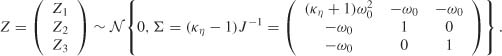
In the proof of Theorem 7.2, we showed that
For any value of θ0 ![]() Θ (even when θ0
Θ (even when θ0 ![]()
![]() ), it will be shown that the vector Zn is well defined and satisfies
), it will be shown that the vector Zn is well defined and satisfies
provided J exists. By contrast, when
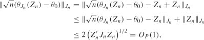
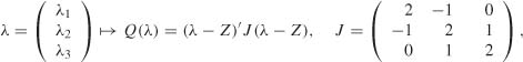
equation (8.4) is no longer valid. However, we will show that the asymptotic distribution of n1/2(![]() − θ0) is well approximated by that of the vector n1/2{θ − θ0) which is located at the minimal distance of Zn, under the constraint θ
− θ0) is well approximated by that of the vector n1/2{θ − θ0) which is located at the minimal distance of Zn, under the constraint θ ![]() Θ. Consider thus a random vector θJn (Jn) (which is not an estimator, of course) solving the minimization problem
Θ. Consider thus a random vector θJn (Jn) (which is not an estimator, of course) solving the minimization problem
It will be shown that Jn converges to the positive definite matrix J. For n large enough, we thus have
where dist Jn (x, y) := {(x − y)′ Jn(x − y)}1/2 is a distance between two points x and y of ![]() p+q+1, and where the distance between a point x and a subset S of
p+q+1, and where the distance between a point x and a subset S of ![]() p+q+1 is defined by dist Jn(x, S) = inf s
p+q+1 is defined by dist Jn(x, S) = inf s![]() sdist Jn(x, S).
sdist Jn(x, S).
We allow θ0 to have null components, but we do not consider the (less interesting) case where θ0 reaches another boundary of Θ. More precisely, we assume that
Bl: ![]() ,
,
where 0 < ![]() <
< ![]() and 0 < min{
and 0 < min{![]() 2, …,
2, …, ![]() p+q+1}. In this case
p+q+1}. In this case ![]() and
and ![]() (
(![]() n − θ0) belong to the local parameter space’
n − θ0) belong to the local parameter space’
where Λ1 = ![]() and, for i = 2,…, p + q + 1, Λi- =
and, for i = 2,…, p + q + 1, Λi- = ![]() if θ0i ≠ 0 and Λi = [0, ∞) if θ0i = 0. With the notation
if θ0i ≠ 0 and Λi = [0, ∞) if θ0i = 0. With the notation
we thus have, with probability 1,
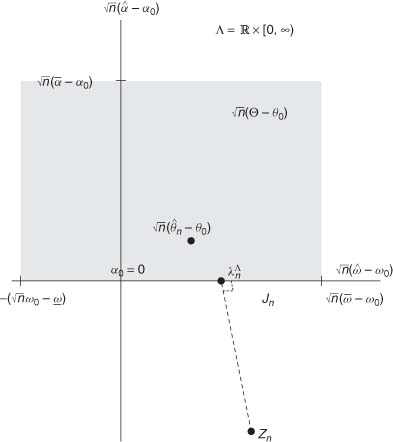
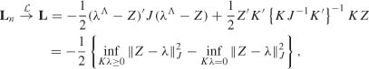
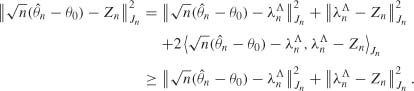
The vector ![]() is the projection of Zn on Λ, with respect to the norm
is the projection of Zn on Λ, with respect to the norm ![]() (see Figure 8.1). Since Λ is closed and convex, such a projection is unique. We will show that
(see Figure 8.1). Since Λ is closed and convex, such a projection is unique. We will show that
Since (Zn, Jn) tends in law to (Z, J) and ![]() is a function of (Zn, Jn) which is continuous everywhere except at the points where Jn is singular (that is, almost everywhere with respect to the distribution of (Z, J) because J is invertible), we have
is a function of (Zn, Jn) which is continuous everywhere except at the points where Jn is singular (that is, almost everywhere with respect to the distribution of (Z, J) because J is invertible), we have ![]() , where λΛ is the solution of limiting problem
, where λΛ is the solution of limiting problem
Figure 8.1 ARCH(l) model with θ0 = (ω0,0) and Θ = [![]() ,
,![]() ] × [0,
] × [0,![]() ]:
]: ![]() (Θ − θ0) = [−
(Θ − θ0) = [− ![]() (ω0 −
(ω0 − ![]() ),
), ![]() (
(![]() − ω0)] × [0,
− ω0)] × [0, ![]() (
(![]() − α0)] is the gray area;
− α0)] is the gray area; ![]()
![]() (
(![]() n − θ0) and
n − θ0) and ![]() have the same asymptotic distribution.
have the same asymptotic distribution.
In addition to Bl, we retain most of the assumptions of Theorem 7.2:
B2: θ0 ![]() Θ and Θ is a compact set.
Θ and Θ is a compact set.
B3: γ(A0) < 0 and for all θ ![]() Θ,
Θ, ![]()
B4: ![]() has a nondegenerate distribution with E
has a nondegenerate distribution with E![]() = 1
= 1
B5: If p > 0, ![]() (z) and
(z) and ![]() (z) do not have common roots,
(z) do not have common roots, ![]() (1)≠ 0, and
(1)≠ 0, and ![]() .
.
B6: κη = E![]() < ∞.
< ∞.
We also need the following moment assumption:
B7: ![]() < ∞
< ∞
When θ0 ![]()
![]() , we can show the existence of the information matrix
, we can show the existence of the information matrix
without moment assumptions similar to B7. The following example shows that, in the ARCH case, this is no longer possible when we allow θ0 ![]() ∂Θ.
∂Θ.
Example 8.1 (The existence of J may require a moment of order 4) Consider the ARCH(2) model
where the true values of the parameters are such that ω0 > 0, α01 ≥ 0, α02 = 0, and the distribution of the iid sequence (η) is defined, for a > 1, by
The process (![]() t) is always stationary, for any value of α01 (since exp {− E(log
t) is always stationary, for any value of α01 (since exp {− E(log ![]() )} = +∞, the strict stationarity constraint (2.10) holds true). By contrast,
)} = +∞, the strict stationarity constraint (2.10) holds true). By contrast, ![]() t does not possess moments of order 2 when α01 ≥ 1 (see Proposition 2.2).
t does not possess moments of order 2 when α01 ≥ 1 (see Proposition 2.2).
We have
so that
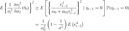
because on the one hand ηt − 1 =0 entails ![]() t − 1 = 0, and on the other hand ηt − 1 and
t − 1 = 0, and on the other hand ηt − 1 and ![]() t − 2 are independent. Consequently, if E
t − 2 are independent. Consequently, if E![]() = ∞ then the matrix J does not exist.
= ∞ then the matrix J does not exist.
We then have the following result.
Theorem 8.1 (QML asymptotic distribution at the boundary) Under assumptions B1–B7, the asymptotic distribution of ![]() (
(![]() n − θ0) is that of λΛ satisfying (8.10), where Λ is given by (8.7).
n − θ0) is that of λΛ satisfying (8.10), where Λ is given by (8.7).
Remark 8.1 (We retrieve the standard results in ![]() ) For θ0
) For θ0 ![]()
![]() , the result is shown in Theorem 7.2. Indeed, in this case Λ =
, the result is shown in Theorem 7.2. Indeed, in this case Λ = ![]() p+q+1 and
p+q+1 and
Theorem 8.1 is thus only of interest when θ0 is at the boundary ∂Θ of the parameter space.
Remark 8,2 (The moment condition B7 can sometimes be relaxed) Apart from the ARCH (q) case, it is sometimes possible to get rid of the moment assumption B7. Note that under the condition γ(A0) < 0, we have ![]() with b00 > 0, b0j≥0. The derivatives ∂
with b00 > 0, b0j≥0. The derivatives ∂![]() /∂θk have the form of similar series. It can be shown that the ratio {∂
/∂θk have the form of similar series. It can be shown that the ratio {∂![]() /∂θ}/
/∂θ}/![]() admits moments of all orders whenever any term
admits moments of all orders whenever any term ![]() −j which appears in the numerator is also present in the denominator. This allows us to show (see the references at the end of the chapter) that, in the theorem, assumption B7 can be replaced by
−j which appears in the numerator is also present in the denominator. This allows us to show (see the references at the end of the chapter) that, in the theorem, assumption B7 can be replaced by
B7:′ b0j > 0 for all j ≥ 1, where ![]() .
.
Note that a sufficient condition for B7′ is α01 > 0 and β01 > 0 (because![]() ). A necessary condition is obviously that α01 > 0 (because b01 = α01). Finally, a necessary and sufficient condition for B7′ is
). A necessary condition is obviously that α01 > 0 (because b01 = α01). Finally, a necessary and sufficient condition for B7′ is
Obviously, according to Example 8.1, assumption B7′ is not satisfied in the ARCH case.
8.2.1 Computation of the Asymptotic Distribution
In this section, we will show how to compute the solutions of (8.10). Switching the components of θ, if necessary, it can be assumed without loss of generality that the vector ![]() of the first d1 components of θ0 has strictly positive elements and that the vector
of the first d1 components of θ0 has strictly positive elements and that the vector ![]() of the last d2 = p + q + 1 − d1 components of θ0 is null. This can be written as
of the last d2 = p + q + 1 − d1 components of θ0 is null. This can be written as
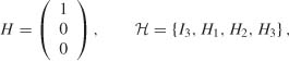
More generally, it will be useful to consider all the subsets of these constraints. Let
be the set of the matrices obtained by deleting no, one, or several (but not all) rows of K. Note that the solution of the constrained minimization problem (8.10) is the unconstrained solution λ = Z when the latter satisfies the constraint, that is, when
When Z ![]() Λ, the solution λΛ coincides with that of an equality constrained problem of the form
Λ, the solution λΛ coincides with that of an equality constrained problem of the form
An important difference, compared to the initial minimization program (8.10), is that the minimization is done here on a vectorial space. The solution is given by a projection (nonorthogonal when J is not the identity matrix). We thus obtain (see Exercise 8.1)
is the projection matrix (orthogonal for the metric defined by J) on the orthogonal subspace of the space generated by the rows of Ki Note that λKi does not necessarily belong to Λ because Kiλ = 0 does not imply that Kλ ≥ 0. Let ![]() = {λKi : Ki
= {λKi : Ki ![]()
![]() and λKi ≥ 0} be the class of the admissible solutions. It follows that the solution that we are looking for is
and λKi ≥ 0} be the class of the admissible solutions. It follows that the solution that we are looking for is
This formula can be used in practice to obtain realizations of λΛ from realizations of Z. The Q(λKi) can be obtained by writing
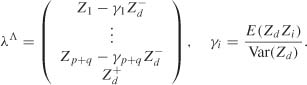
Another expression (of theoretical interest) for λΛ is
where ![]() 0 = Λ and the
0 = Λ and the ![]() i form a partition of
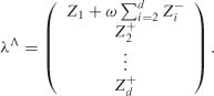
i form a partition of ![]() p+q+1. Indeed, according to the zone to which Z belongs, a solution λΛ = λKi is obtained. We will make explicit these formulas in a few examples. Let d = p + q + 1, z+ = z
p+q+1. Indeed, according to the zone to which Z belongs, a solution λΛ = λKi is obtained. We will make explicit these formulas in a few examples. Let d = p + q + 1, z+ = z ![]() (0,+∞)(z) and z− = z
(0,+∞)(z) and z− = z ![]() (−∞,0) (z).
(−∞,0) (z).
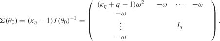
Example 8.2 (Law when only one component is at the boundary) When d2 = 1, that is, when only the last component of θ0 is zero, we have
and
We finally obtain
where c is the last column of J−1 divided by the (d, d)th element of this matrix. Note that the last component of λΛ is ![]() . Noting that J−1 is, up to a multiplicative factor, the variance of Z, it can also be seen that
. Noting that J−1 is, up to a multiplicative factor, the variance of Z, it can also be seen that
Thus ![]() if and only if Cov(Zi, Zd) = 0.
if and only if Cov(Zi, Zd) = 0.
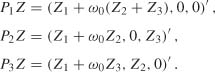
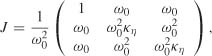
Example 8.3 (ARCH(2) model when the data generating process is a white noise) Consider an ARCH(2) model with θ0 = (ω0, 0, 0). We thus have d2 = 2, d1 = 1 and
with K1 = K, K2 = (0, 1, 0) and K3 = (0, 0, 1). Exercise 8.6 shows that
Using K Σ K′ = I2 and KiΣK′i for i = 2, 3 in particular, we thus obtain
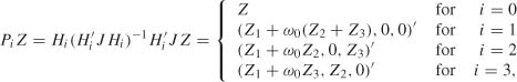
Let P0 = I3 and K0 = 0. Using (8.14), we have
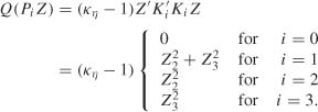
This shows that
In order to obtain a slightly simpler expression for the projections defined in (8.13), note that the constraint (8.12) can again be written as
We define a dual of ![]() , by
, by
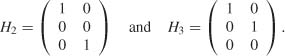
the set of the matrices obtained by deleting from 0 to d2 of the last d2 columns of the matrix Id. Note that the elements of ![]() can always be numbered in such a way that H0 = Id corresponds to the absence of constraint on θ0 and that, for
can always be numbered in such a way that H0 = Id corresponds to the absence of constraint on θ0 and that, for ![]() , the constraint Kiθ0 = 0 corresponds to the constraint θ0 = HiH′iθ0. Exercise 8.2 then shows that
, the constraint Kiθ0 = 0 corresponds to the constraint θ0 = HiH′iθ0. Exercise 8.2 then shows that
for ![]() (with P0 = Id). Note that (8.18) requires the inversion of only one matrix of size (d − k) × (d − k) (d − k being the number of columns of Hi), whereas (8.13) requires the inversion of one matrix of size d × d and another matrix of size k × k. To illustrate this new formula, we return to our previous examples.
(with P0 = Id). Note that (8.18) requires the inversion of only one matrix of size (d − k) × (d − k) (d − k being the number of columns of Hi), whereas (8.13) requires the inversion of one matrix of size d × d and another matrix of size k × k. To illustrate this new formula, we return to our previous examples.
Example 8,4 (Example 8.2 continued) We have
and
using the notation
where the matrix J11 is of size d1 × d1, the vectors J12 = J′1 and (1) are of size d1 × 1, and J22 and Z(2) = Zd are scalars. We finally obtain
which can be shown using (8.15) and
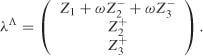
Example 8.5 (Example 83 continued) We have
with H1 = H
In view of Exercise 8.6, we have
which allows us to obtain
and to retrieve (8.16). Note that, in this example, the calculation are simpler with (8.13) than with (8.18), because J−1 has a simpler expression than J.
8.3 Significance of the GARCH Coefficients
We make the assumptions of Theorem 8.1 and use the notation of Section 8.2.1. Assume ![]() and consider the testing problem
and consider the testing problem
Recall that under H0, we have
where the distribution of λΛ is defined by
with ![]()
8.3.1 Tests and Rejection Regions
For parametric assumptions of the form (8.19), the most popular tests are the Wald, score and likelihood ratio tests.
The Wald test looks at whether ![]() is close to 0. The usual Wald statistic is defined by
is close to 0. The usual Wald statistic is defined by
where ![]() is a consistent estimator of Σ = (κη − 1)J−1.
is a consistent estimator of Σ = (κη − 1)J−1.
Score (or Lagrange Multiplier or Rao) Statistic
Let
denote the QMLE of θ constrained by θ(2) = 0. The score test aims to determine whether ∂In (![]() n|2)/∂θ is not too far from 0, using a statistic of the form
n|2)/∂θ is not too far from 0, using a statistic of the form
where ![]() η|2 and
η|2 and ![]() n|2 denote consistent estimators of κη and J.
n|2 denote consistent estimators of κη and J.
Likelihood Ratio Statistic
The likelihood ratio test is based on the fact that under H0 : θ(2) = 0, the constrained (quasi) log-likelihood log Ln (![]() n|2) = − (n/2)
n|2) = − (n/2)![]() n(
n(![]() n|2) should not be much smaller than the unconstrained log-likelihood − (n/2)
n|2) should not be much smaller than the unconstrained log-likelihood − (n/2)![]() n(
n(![]() n). The test employs the statistic
n). The test employs the statistic
Usual Rejection Regions
From the practical viewpoint, the score statistic presents the advantage of only requiring constrained estimation, which is sometimes much simpler than the unconstrained estimation required by the two other tests. The likelihood ratio statistic does not require estimation of the information matrix J, nor the kurtosis coefficient κη. For each test, it is clear that the null hypothesis must be rejected for large values of the statistic. For standard statistical problems, the three statistics asymptotically follow the same ![]() distribution under the null. At the asymptotic level α, the standard rejection regions are thus
distribution under the null. At the asymptotic level α, the standard rejection regions are thus
where ![]() , (l − α) is the (1 − α)-quantile of the χ2 distribution with d2 degrees of freedom. In the case d2 = 1, for testing the significance of only one coefficient, the most widely used test is Student’s t test, defined by the rejection region
, (l − α) is the (1 − α)-quantile of the χ2 distribution with d2 degrees of freedom. In the case d2 = 1, for testing the significance of only one coefficient, the most widely used test is Student’s t test, defined by the rejection region
where ![]() . This test is equivalent to the standard Wald test because
. This test is equivalent to the standard Wald test because ![]() (tn being here always positive or null, because of the positivity constraints of the QML estimates) and
(tn being here always positive or null, because of the positivity constraints of the QML estimates) and
Our testing problem is not standard because, by Theorem 8.1, the asymptotic distribution of ![]() n is not normal. We will see that, among the previous rejection regions, only that of the score test asymptotically has the level α.
n is not normal. We will see that, among the previous rejection regions, only that of the score test asymptotically has the level α.
8.3.2 Modification of the Standard Tests
The following proposition shows that for the Wald and likelihood ratio tests, the asymptotic distribution is not the usual ![]() under the null hypothesis. The proposition also shows that the asymptotic distribution of the score test remains the
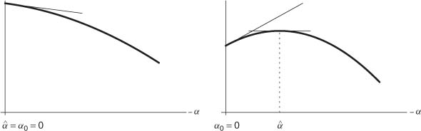
under the null hypothesis. The proposition also shows that the asymptotic distribution of the score test remains the ![]() distribution. The asymptotic distribution of Rn is not affected by the fact that, under the null hypothesis, the parameter is at the boundary of the parameter space. These results are not very surprising. Take the example of an ARCH(l) with the hypothesis H0:α0 = 0 of absence of ARCH effect. As illustrated by Figure 8.2, there is a nonzero probability that
distribution. The asymptotic distribution of Rn is not affected by the fact that, under the null hypothesis, the parameter is at the boundary of the parameter space. These results are not very surprising. Take the example of an ARCH(l) with the hypothesis H0:α0 = 0 of absence of ARCH effect. As illustrated by Figure 8.2, there is a nonzero probability that ![]() be at the boundary, that is, that
be at the boundary, that is, that ![]() = 0. Consequently Wn = n
= 0. Consequently Wn = n![]() 2 admits a mass at 0 and does not follow, even asymptotically, the
2 admits a mass at 0 and does not follow, even asymptotically, the ![]() law. The same conclusion can be drawn for the likelihood ratio test. On the contrary, the score nl/2∂ln(θ0)/∂θ can take as well positive or negative values, and does not seem to have a specific behavior when θ0 is at the boundary.
law. The same conclusion can be drawn for the likelihood ratio test. On the contrary, the score nl/2∂ln(θ0)/∂θ can take as well positive or negative values, and does not seem to have a specific behavior when θ0 is at the boundary.
Proposition 83 (Asymptotic distribution of the three statistics under H0) Under H0 and the assumptions of Theorem 8.1,
where Ω = K′ {(κη − 1) KJ−1 K′}−1 K and λΛ satisfies (8.20).
Figure 8.2 Concentrated log4ikelihood (solid line) α ![]() log Ln(
log Ln(![]() , α) for an ARCH(l) model. Assume there is no ARCH effect: the true value of the ARCH parameter is α0 = 0- In the configuration on the right, the likelihood maximum does not lie at the boundary and the three statistics Wn, Rn and Ln take strictly positive values. In the configuration on the left, we have Wn = n
, α) for an ARCH(l) model. Assume there is no ARCH effect: the true value of the ARCH parameter is α0 = 0- In the configuration on the right, the likelihood maximum does not lie at the boundary and the three statistics Wn, Rn and Ln take strictly positive values. In the configuration on the left, we have Wn = n![]() 2 = 0 and Ln = 2 {log Ln(
2 = 0 and Ln = 2 {log Ln(![]() ,
, ![]() ) − log Ln(a), 0)} = 0, whereas Rn = {∂ log Ln(
) − log Ln(a), 0)} = 0, whereas Rn = {∂ log Ln(![]() , 0)/∂ α}2 continues to take a strictly positive value.
, 0)/∂ α}2 continues to take a strictly positive value.
Remark 8.3 (Equivalence of the statistics Wn and Ln) Let ![]() η be an estimator which converges in probability to κη. We can show that
η be an estimator which converges in probability to κη. We can show that
under the null hypothesis. The Wald and likelihood ratio tests will thus have the same asymptotic critical values, and will have the same local asymptotic powers (see Exercises 8.8 and 8.9, and Section 8.3.4). They may, however, have different asymptotic behaviors under nonlocal alternatives.
Remark 8.4 (Assumptions on the tests) In order for the Wald statistic to be well defined, Ω must exist, that is, J = J (θ0) must exist and must be invertible. This is not the case, in particular, for a GARCH(p, q) at θ0 = (ω0, 0, …, 0), when p ≠ 0. It is thus impossible to carry out a Wald test on the simultaneous nullity of all the αi and βi coefficients in a GARCH(p, q), p ≠ 0. The assumptions of Theorem 8.1 are actually required, in particular the identifiability assumptions. Iti is thus impossible to test, for instance, an ARCH(l) against a GARCH(2, 1), but we can test, for instance, an ARCH(l) against an ARCH(3).
A priori, the asymptotic distributions W and L depend on J, and thus on nuisance parameters. We will consider two particular cases: the case where we test the nullity of only one GARCH coefficient and the case where we test the nullity of all the coefficients of an ARCH. In the two cases the asymptotic laws of the test statistics are simpler and do not depend on nuisance parameters. In the second case, both the test statistics and their asymptotic laws are simplified.
8.3.3 Test for the Nullity of One Coefficient
Consider the case d1 = 1, which is perhaps the most interesting case and corresponds to testing the nullity of only one coefficient. In view of (8.15), the last component of λΛ is equal to ![]() . We thus have
. We thus have
where Z* ~ ![]() (0, 1). Using the symmetry of the Gaussian distribution, and the independence between Z*2 and
(0, 1). Using the symmetry of the Gaussian distribution, and the independence between Z*2 and ![]() {z*>0} when z* follows the real normal law, we obtain
{z*>0} when z* follows the real normal law, we obtain
Testing
can thus be achieved by using the critical region ![]() at the asymptotic level α ≤ 1/2. In view of Remark 8.3, we can define a modified likelihood ratio test of critical region
at the asymptotic level α ≤ 1/2. In view of Remark 8.3, we can define a modified likelihood ratio test of critical region ![]() . Note that the standard Wald test
. Note that the standard Wald test ![]() has the asymptotic level α/2, and that the asymptotic level of the standard likelihood ratio test
has the asymptotic level α/2, and that the asymptotic level of the standard likelihood ratio test ![]() is much larger than α when the kurtosis coefficient κΛ is large. A modified version of the Student t test is defined by the rejection region
is much larger than α when the kurtosis coefficient κΛ is large. A modified version of the Student t test is defined by the rejection region
We observe that commercial software - such as GAUSS, R, RATS, SAS and SPSS - do not use the modified version (8.25), but the standard version (8.21). This standard test is not of asymptotic level α but only α/2. To obtain a t test of asymptotic level α it then suffices to use a test of nominal level 2α.
Example 8.6 (Empirical behavior of the tests under the null) We simulated 5000 independent samples of length n = 100 and n = 1000 of a strong ![]() (0, 1) white noise. On each realization we fitted an ARCH(l) model
(0, 1) white noise. On each realization we fitted an ARCH(l) model ![]() , by QML, and carried out tests of H0 : α = 0 against H1 : α > 0.
, by QML, and carried out tests of H0 : α = 0 against H1 : α > 0.
We began with the modified Wald test with rejection region
This test is of asymptotic level 5%. For the sample size n = 100, we observed a relative rejection frequency of 6.22%. For n = 1000, we observe a relative rejection frequency of 5.38%, which is not significantly different from the theoretical 5%. Indeed, an elementary calculation shows that, on 5000 independent replications of a same experiment with success probability 5%, the success percentage should vary between 4.4% and 5.6% with a probability of approximately 95%. Figure 8.3 shows that the empirical distribution of Wn is quite close to the asymptotic distribution ![]() , even for the small sample size n = 100.
, even for the small sample size n = 100.
We then carried out the score test defined by the rejection region
where R2 is the determination coefficient of the regression of ![]() on 1 and
on 1 and ![]() This test is also of asymptotic level 5%. For the sample size n = 100, we observed a relative rejection frequency of 3.40%. For n = 1000, we observed a relative frequency of 4.32%.
This test is also of asymptotic level 5%. For the sample size n = 100, we observed a relative rejection frequency of 3.40%. For n = 1000, we observed a relative frequency of 4.32%.
We also used the modified likelihood ratio test. For the sample size n = 100, we observed a relative rejection frequency of 3.20%, and for n = 1000 we observed 4.14%.
On these simulation experiments, the Type I error is thus slightly better controlled by the modified Wald test than by the score and modified likelihood ratio tests.
Example 8.7 (Comparison of the tests under the alternative hypothesis) We implemented the Wn, Rn and Ln tests of the null hypothesis H0 : α01 = 0 in the ARCH(l) model
Figure 8.3 Comparison between a kernel density estimator of the Wald statistic (dotted line) and the ![]() density on [0.5, ∞) (solid line) on 5000 simulations of an ARCH(l) process with α01 = 0: (left) for sample size n = 100; (right) for n = 1000.
density on [0.5, ∞) (solid line) on 5000 simulations of an ARCH(l) process with α01 = 0: (left) for sample size n = 100; (right) for n = 1000.
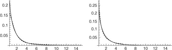
Figure 8.4 Comparison of the observed powers of the Wald test (thick line), of the score test (dotted line) and of the likelihood ratio test (thin line), as function of the nominal level α, on 5000 simulations of an ARCH(l) process: (left) for n = 100 and α01 = 0.2; (right) for n = 1000 and α01 = 0.05.
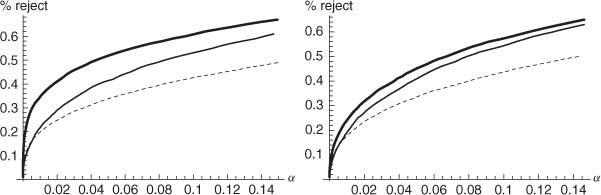
![]() compares the observed powers of the three tests, that is, the relative frequency of rejection of the hypothesis H0 that there is no ARCH effect, on 5000 independent realizations of length n = 100 and n = 1000 of an ARCH(l) model with α01 = 0.2 when n = 100, and α01 = 0.05 when n = 1000. On these simulated series, the modified Wald test turns out to be the most powerful.
compares the observed powers of the three tests, that is, the relative frequency of rejection of the hypothesis H0 that there is no ARCH effect, on 5000 independent realizations of length n = 100 and n = 1000 of an ARCH(l) model with α01 = 0.2 when n = 100, and α01 = 0.05 when n = 1000. On these simulated series, the modified Wald test turns out to be the most powerful.
8.3.4 Conditional Homoscedastlclty Tests with ARCH Models
Another interesting case is that obtained with d1 = 1, θ(1) = ω, p = 0 and d2 = q. This case corresponds to the test of the conditional homoscedasticity null hypothesis
in an ARCH(q) model
We will see that for testing (8.26) there exist very simple forms of the Wald and score statistics.
Simplified Form of the Wald Statistic
Using Exercise 8.6, we have
Since KΣK′ = Iq, we obtain a very simple form for the Wald statistic:
Asymptotic Distribution W and L
A trivial extension of Example 83 yields
The asymptotic distribution of ![]() is thus that of
is thus that of
where the Zi are independent ![]() (0, 1). Thus, in the case where an ARCH(q) is fitted to a white noise we havei
(0, 1). Thus, in the case where an ARCH(q) is fitted to a white noise we havei
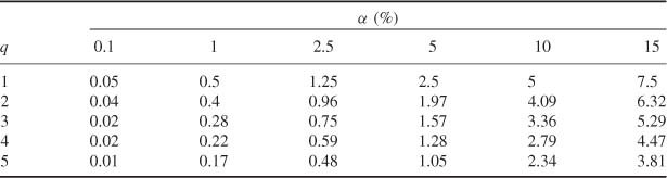
This asymptotic distribution is tabulated and the critical values are given in Table 8.2. In view of Remark 8.3, Table 8.2 also yields the asymptotic critical values of the modified likelihood ratio statistic 2Ln/(![]() − 1). Table 8.3 shows that the use of the standard
− 1). Table 8.3 shows that the use of the standard ![]() -based critical values of the Wald test would lead to large discrepancies between the asymptotic levels and the nominal level α.
-based critical values of the Wald test would lead to large discrepancies between the asymptotic levels and the nominal level α.
Table 8.2 Asymptotic critical value Cqα, at level α, of the Wald test of rejection region ![]() for the conditional homoscedasticity hypothesis H0 : α1 = … = αq = 0 in an ARCH (q) model.
for the conditional homoscedasticity hypothesis H0 : α1 = … = αq = 0 in an ARCH (q) model.
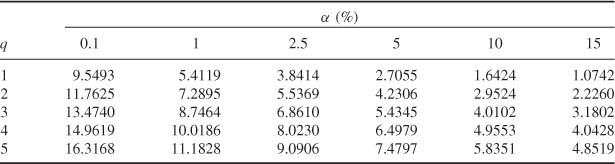
Table 8.3 Exact asymptotic level (%) of erroneous Wald tests, of rejection region ![]() , under the conditional homoscedasticity assumption H0 : α1 = … = αq = 0 in an ARCH(q) model.
, under the conditional homoscedasticity assumption H0 : α1 = … = αq = 0 in an ARCH(q) model.
For the hypothesis (8.26) that all the α coefficients of an ARCH(q) model are equal to zero, the score statistic Rn can be simplified. To work within the linear regression framework, write
where Y is the vector of length n of the ‘dependent’ variable 1 − ![]() /
/![]() , where X is the n × (q × 1) matrix of the constant
, where X is the n × (q × 1) matrix of the constant ![]() (in the first column) and of the ‘explanatory’ variables
(in the first column) and of the ‘explanatory’ variables ![]() (in column i + 1, with the convention
(in column i + 1, with the convention ![]() t = 0 for t ≤ 0), and
t = 0 for t ≤ 0), and ![]() . Estimating J(θ0) by n−1 X′X and κη − 1 by n−1Y′Y, we obtain
. Estimating J(θ0) by n−1 X′X and κη − 1 by n−1Y′Y, we obtain
and one recognizes n times the coefficient of determination in the linear regression of Y on the columns of X. Since this coefficient is not changed by linear transformation of the variables (see Exercise 5.11), we simply have Rn = nR2, where R2 is the coefficient of determination in the regression of ![]() on a constant and q lagged values
on a constant and q lagged values ![]() . Under the null hypothesis of conditional homoscedasticity, Rn asymptotically follows the
. Under the null hypothesis of conditional homoscedasticity, Rn asymptotically follows the ![]() law.
law.
The previous simple forms of the Wald and score tests are obtained with estimators of J which exploit the particular form of the matrix under the null. Note that there exist other versions of these tests, obtained with other consistent estimators of J. The different versions are equivalent under the null, but can have different asymptotic behaviors under the alternative.
8.3.5 Asymptotic Comparison of the Tests
The Wald and score tests that we have just defined are in general consistent, that is, their powers converge to 1 when they are applied to a wide class of conditionally heteroscedastic processes. An asymptotic study will be conducted via two different approaches: Bahadur’s approach compares the rates of convergence to zero of the p-values under fixed alternatives, whereas Pitman’s approach compares the asymptotic powers under a sequence of local alternatives, that is, a sequence of alternatives tending to the null as the sample size increases.
Bahadur’s Approach
Let Sw(t) = ![]() (W > t) and SR(t =
(W > t) and SR(t = ![]() (R > t) be the asymptotic survival functions of the two test statistics, under the null hypothesis H0 defined by (8.26). Consider, for instance, the Wald test. Under the alternative of an ARCH(q) which does not satisfy H0, the p-value of the Wald test Sw(Wn) converges almost surely to zero as n → ∞ because
(R > t) be the asymptotic survival functions of the two test statistics, under the null hypothesis H0 defined by (8.26). Consider, for instance, the Wald test. Under the alternative of an ARCH(q) which does not satisfy H0, the p-value of the Wald test Sw(Wn) converges almost surely to zero as n → ∞ because
The p-value of a test is typically equivalent to exp{−nc/2}, where c is a positive constant called the Bahadur slope. Using the fact that
and that ![]() , the (approximate1) Bahadur slope of the Wald test is thus
, the (approximate1) Bahadur slope of the Wald test is thus
To compute the Bahadur slope of the score test, note that we have the linear regression model ![]() = ω +
= ω + ![]() (B)
(B)![]() + vt, where vt = (
+ vt, where vt = (![]() − 1)
− 1)![]() (θ0) is the linear innovation of
(θ0) is the linear innovation of ![]() . We then have
. We then have
The previous limit is thus equal to the Bahadur slope of the score test. The comparison of the two slopes favors the score test over the Wald test.
Proposition 8.4 Let (![]() t) be a strictly stationary and nonanticipative solution of the ARCH(q) model (8.27), with E(
t) be a strictly stationary and nonanticipative solution of the ARCH(q) model (8.27), with E(![]() ) < ∞ and
) < ∞ and ![]() . The score test is considered as more efficient than the Wald test in Bahadur’s sense because its slope is always greater or equal to that of the Wald test, with equality when q = 1.
. The score test is considered as more efficient than the Wald test in Bahadur’s sense because its slope is always greater or equal to that of the Wald test, with equality when q = 1.
Example 8.8 (Slopes In the ARCH(l) and ARCH(2) cases) The slopes are the same in the ARCH(l) case because
In the ARCH(2) case with fourth-order moment, we have
We see that the second limit is always larger than the first. Consequently, in Bahadur’s sense, the Wald and Rao tests have the same asymptotic efficiency in the ARCH(l) case. In the ARCH(2) case, the score test is, still in Bahadur’s sense, asymptotically more efficient than the Wald test for testing the conditional homoscedasticity (that is, α1 = α2 = 0).
Bahadur’s approach is sometimes criticized for not taking account of the critical value of test, and thus for not really comparing the powers. This approach only takes into account the (asymptotic) distribution of the statistic under the null and the rate of divergence of the statistic under the alternative. It is unable to distinguish a two-sided test from its one-sided counterpart (see Exercise 8.8). In this sense the result of Proposition 8.4 must be put into perspective.
Pitman’s Approach
In the ARCH(l) case, consider a sequence of local alternatives Hn(τ) : α1= τ/![]() . We can show that under this sequence of alternatives,
. We can show that under this sequence of alternatives,
Consequently, the local asymptotic power of the Wald test is
The score test has the local asymptotic power
Note that (8.32) Is the power of the test of the assumption H0 : θ = 0 against the assumption H1 : θ = τ > 0, based on the rejection region of {X > c1] with only one observation X ~ ![]() (θ, 1). The power (8.33) is that of the two-sided test {|X| > c2}. The tests {X > c1} and {|X| > c2} have the same level, but the first test Is uniformly more powerful than the second (by the Neyman-Pearson lemma, {|X| > c1} is even uniformly more powerful than any test of level less than or equal to α, for any one-sided alternative of the form H1). The local asymptotic power of the Wald test Is thus uniformly strictly greater than that of Rao’s test for testing for conditional homoscedasticity in an ARCH(l) model.
(θ, 1). The power (8.33) is that of the two-sided test {|X| > c2}. The tests {X > c1} and {|X| > c2} have the same level, but the first test Is uniformly more powerful than the second (by the Neyman-Pearson lemma, {|X| > c1} is even uniformly more powerful than any test of level less than or equal to α, for any one-sided alternative of the form H1). The local asymptotic power of the Wald test Is thus uniformly strictly greater than that of Rao’s test for testing for conditional homoscedasticity in an ARCH(l) model.
Consider the ARCH(2) case, and a sequence of local alternatives Hn(τ) : α1 = τ1/![]() , α2 = τ2/
, α2 = τ2/ ![]() . Under this sequence of alternatives
. Under this sequence of alternatives
with (U1, U2)′ ~ ![]() (0, I2). Let c1 be the critical value of the Wald test of level α. The local asymptotic power of the Wald test is
(0, I2). Let c1 be the critical value of the Wald test of level α. The local asymptotic power of the Wald test is
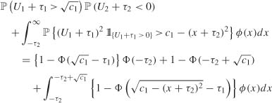
Let c2 be the critical value of the Rao test of level α. The local asymptotic power of the Rao test is
where (U1 + ω1)2 + (U2 + ω1)2 follows a noncentral χ2 distribution, with two degrees of freedom and noncentrailty parameter ![]() . Figure 8.5 compares the powers of the two tests when ω1 = ω2.
. Figure 8.5 compares the powers of the two tests when ω1 = ω2.
Figure 8.5 Local asymptotic power of the Wald test (solid line) and of the Rao test (dotted line) for testing for conditional homoscedasticity in an ARCH(2) model.
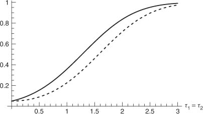
Thus, the comparison of the local asymptotic powers clearly favors the Wald test over the score test, counterbalancing the result of Proposition 8.4.
8.4 Diagnostic Checking with Portmanteau Tests
To check the adequacy of a given time series model, for instance an ARMA(p, q) model, it is common practice to test the significance of the residual autocorrelations. In the GARCH framework this approach is not relevant because the process ![]() t =
t = ![]() t/
t/![]() t is always a white noise (possibly a martingale difference) even when the volatility is misspecified, that is, when
t is always a white noise (possibly a martingale difference) even when the volatility is misspecified, that is, when ![]() with
with ![]() . To check the adequacy of a volatility model, for instance a GARCH(p, q) of the form (7.1), it is much more fruitful to look at the squared residual autocovariances
. To check the adequacy of a volatility model, for instance a GARCH(p, q) of the form (7.1), it is much more fruitful to look at the squared residual autocovariances
where |h| < n, ![]() t =
t = ![]() t(
t(![]() n) is defined by (7.4) and
n) is defined by (7.4) and ![]() n is the QMLE given by (7.9).
n is the QMLE given by (7.9).
For any fixed integer m, 1 ≤ m < n, consider the statistic ![]() m = (
m = (![]() (1),…,
(1),…,![]() (m))′. Let
(m))′. Let ![]() η and
η and ![]() be weakly consistent estimators of κη and J. For instance, one can take
be weakly consistent estimators of κη and J. For instance, one can take
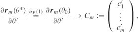
Define also the m × (p + q + 1) matrix ![]() m whose (h, k)th element, for 1 ≤ h ≤ m and 1 ≤ k < p + q + 1, is given by
m whose (h, k)th element, for 1 ≤ h ≤ m and 1 ≤ k < p + q + 1, is given by
Theorem 8.2 (Asymptotic distribution of a portmanteau test statistic) Under the assumptions of Theorem 7.2 ensuring the consistency and asymptotic normality of the QMLE,
with ![]()
The adequacy of the GARCH(p, q) model is rejected at the asymptotic level α when
8.5 Application: Is the GARCH(1, 1) Model Overrepresented?
The GARCH(1, 1) model is by far the most widely used by practitioners who wish to estimate the volatility of daily returns. In general, this model is chosen a priori, without implementing any statistical identification procedure. This practice is motivated by the common belief that the GARCH(1, 1) (or its simplest asymmetric extensions) is sufficient to capture the properties of financial series and that higher-order models may be unnecessarily complicated.
We will show that, for a large number of series, this practice is not always statistically justified. We consider daily and weekly series of 11 returns (CAC, DAX, DJA, DJI, DJT, DJU, FTSE, Nasdaq, Nikkei, SMI and S&P 500) and five exchange rates. The observations cover the period from January 2, 1990 to January 22, 2009 for the daily returns and exchange rates, and from January 2, 1990 to January 20, 2009 for the weekly returns (except for the indices for which the first observations are after 1990). We begin with the portmanteau tests defined in Section 8.4. Table 8.4 shows that the ARCH models (even with large order q) are generally rejected, whereas the GARCH(1, 1) is only occasionally rejected. This table only concerns the daily returns, but similar conclusions hold for the weekly returns and exchange rates. The portmanteau tests are known to be omnibus tests, powerful for a broad spectrum of alternatives. As we will now see, for the specific alternatives for which they are built, the tests defined in Section 8.3 (Wald, score and likelihood ratio) may be much more powerful.
The GARCH(1, 1) model is chosen as the benchmark model, and is successively tested against the GARCH(1, 2), GARCH(1, 3), GARCH(1, 4) and GARCH(2, 1) models. In each case, the three tests (Wald, score and likelihood ratio) are applied. The empirical p-values are displayed in Table 8.5. This table shows that: (i) the results of the tests strongly depend on the alternative;
Table 8.4 Portmanteau test p-values for adequacy of the ARCH(5) and GARCH(1, 1) models for daily returns of stock market indices, based on m squared residual autocovariances. p-values less than 5% are in bold, those less than 1% are underlined.
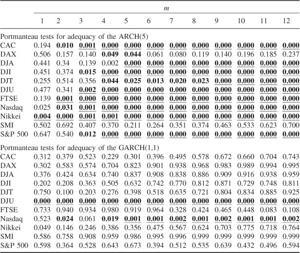
Table 8.5 p-values for tests of the null of a GARCH(1,1) model against the GARCH(1,2), GARCH(1,3), GARCH(1,4) and GARCH(2,1) alternatives, for returns of stock market indices and exchange rates, p-values less than 5% are in bold, those less than 1% are underlined.
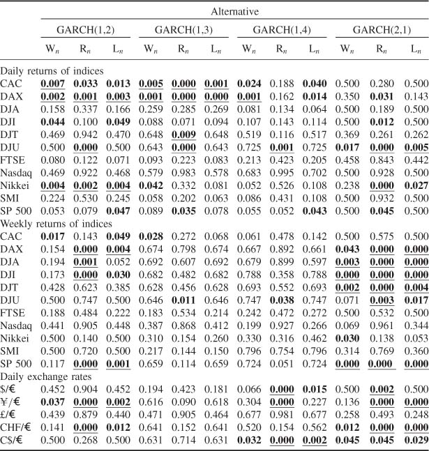
(ii) the p-values of the three tests can be quite different; (iii) for most of the series, the GARCH(1,1) model is clearly rejected. Point (ii) is not surprising because the asymptotic equivalence between the three tests is only shown under the null hypothesis or under local alternatives. Moreover, because of the positivity constraints, it is possible (see, for instance, the DJU) that the estimated GARCH(1,2) model satisfies ![]() 2 = 0 with
2 = 0 with ![]() . In this case, when the estimators lie at the boundary of the parameter space and the score is strongly positive, the Wald and LR tests do not reject the GARCH(1,1) model, whereas the score does reject it. In other situations, the Wald or LR test rejects the GARCH(1,1) whereas the score does not (see, for instance, the DAX for the GARCH(1,4) alternative). This study shows that it is often relevant to employ several tests and several alternatives. The conservative approach of Bonferroni (rejecting if the minimal/?-value multiplied by the number of tests is less than a given level α), leads to rejection of the GARCH(1, 1) model for 16 out of the 24 series in Table 8.5. Other procedures, less conservative than that of Bonferroni, could also be applied (see Wright, 1992) without changing the general conclusion.
. In this case, when the estimators lie at the boundary of the parameter space and the score is strongly positive, the Wald and LR tests do not reject the GARCH(1,1) model, whereas the score does reject it. In other situations, the Wald or LR test rejects the GARCH(1,1) whereas the score does not (see, for instance, the DAX for the GARCH(1,4) alternative). This study shows that it is often relevant to employ several tests and several alternatives. The conservative approach of Bonferroni (rejecting if the minimal/?-value multiplied by the number of tests is less than a given level α), leads to rejection of the GARCH(1, 1) model for 16 out of the 24 series in Table 8.5. Other procedures, less conservative than that of Bonferroni, could also be applied (see Wright, 1992) without changing the general conclusion.
In conclusion, this study shows that the GARCH(1, 1) model is certainly overrepresented in empirical studies. The tests presented in this chapter are easily implemented and lead to selection of GARCH models that are more elaborate than the GARCH(1,1).
8.6 Proofs of the Main Results*
Proof of Theorem 8.1
We will split the proof into seven parts.
(a) Asymptotic normality of score vector. When θ0 ![]() ∂Θ, the function
∂Θ, the function ![]() (θ) can take negative values in a neighborhood of θ0, and
(θ) can take negative values in a neighborhood of θ0, and ![]() t(θ) =
t(θ) = ![]() /
/![]() (θ) + log
(θ) + log ![]() (θ) is then undefined in this neighborhood. Thus the derivative of
(θ) is then undefined in this neighborhood. Thus the derivative of ![]() t(·) does not exist at θ0- By contrast the right derivatives exist, and the vector ∂
t(·) does not exist at θ0- By contrast the right derivatives exist, and the vector ∂![]() t(θ0)/∂θ of the right partial derivatives is written as an ordinary derivative. The same convention is used for the higher-order derivatives, as well as for the right derivatives of ln,
t(θ0)/∂θ of the right partial derivatives is written as an ordinary derivative. The same convention is used for the higher-order derivatives, as well as for the right derivatives of ln, ![]() t and
t and ![]() n at θ0 With these conventions, the formulas for the derivative of criterion remain valid:
n at θ0 With these conventions, the formulas for the derivative of criterion remain valid:
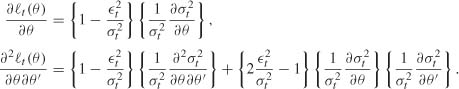
It is then easy to see that J = E∂2![]() t(θ0)/∂θ∂θ′ exists under the moment assumption B7. The ergodic theorem immediately yields
t(θ0)/∂θ∂θ′ exists under the moment assumption B7. The ergodic theorem immediately yields
where J is invertible, by assumptions B4 and B5 (cf. Proof of Theorem 7.2). The convergence (8.5) then directly follows from Slutsky’s lemma and the central limit theorem given in Corollary A.l.
(b) Uniform integrability and continuity of the second-order derivatives. It will be shown that, for all ε > 0, there exists a neighborhood ![]() (θ0) of θ0 such that, almost surely,
(θ0) of θ0 such that, almost surely,
and
Using elementary derivative calculations and the compactness of Θ, it can be seen that
where K > 0 and 0 < ρ < 1. Since supθ![]() Θ, assumption B7 then entails that
Θ, assumption B7 then entails that
In view of (8.34), the Holder and Minkowski inequalities then show (8.36) for all neighborhood of θ0 The ergodic theorem entails that
This expectation decreases to 0 when the neighborhood ![]() (θ0) decreases to the singleton {θ0}, which shows (8.37).
(θ0) decreases to the singleton {θ0}, which shows (8.37).
(c) Convergence in probability of ![]() to θ0 at rate
to θ0 at rate ![]() . In view of (8.35), for n large enough,
. In view of (8.35), for n large enough, ![]() defines a norm. The definition (8.6) of
defines a norm. The definition (8.6) of ![]() entails that
entails that ![]() . The triangular inequality then implies that
. The triangular inequality then implies that
where the last equality comes from the convergence in law of (Zn, Jn) to (Z, J). This entails that ![]() .
.
(d) Quadratic approximation of the objective function. A Taylor expansion yields
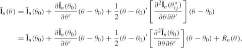
where
and ![]() is between θ and θ0. Note that (8.37) implies that, for any sequence (θn) such that θn − θ0 = OP(1), we have Rn(θn) = oP (
is between θ and θ0. Note that (8.37) implies that, for any sequence (θn) such that θn − θ0 = OP(1), we have Rn(θn) = oP (![]() θn − θ0
θn − θ0![]() 2)- In particular, in view of (c), we have Rn {θJn(Zn)} = oP(n−1). Introducing the vector Zn defined by (8.3), we can write
2)- In particular, in view of (c), we have Rn {θJn(Zn)} = oP(n−1). Introducing the vector Zn defined by (8.3), we can write
where
The initial conditions are asymptotically negligible, even when the parameter stays at the boundary. Result (d) of page 160 remaining valid, we have ![]() for any sequence (θn) such that θn → θ0 in probability.
for any sequence (θn) such that θn → θ0 in probability.
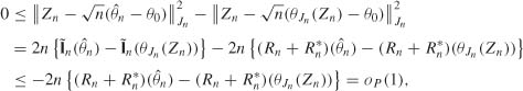
(e) Convergence In probability of ![]() n to θ0 at rate n1/2. We know that
n to θ0 at rate n1/2. We know that
when θ0 ![]()
![]() . We will show that this result remains valid when θ0
. We will show that this result remains valid when θ0 ![]() ∂Θ. Theorem 7.1 applies. In view of (d), the almost sure convergence of
∂Θ. Theorem 7.1 applies. In view of (d), the almost sure convergence of ![]() n to θ0 and of Ji to the nonsingular matrix J, we have
n to θ0 and of Ji to the nonsingular matrix J, we have
and
Since ![]() n(·) is minimized at
n(·) is minimized at ![]() n, we have
n, we have
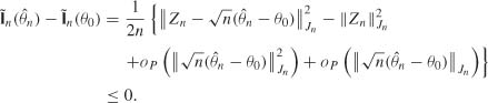
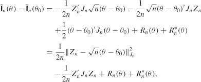
It follows that
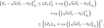
where the last inequality follows from ![]() . The triangular inequality then yields
. The triangular inequality then yields
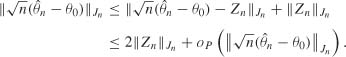
Thus ![]()
where the first line comes from the definition of ![]() , the second line comes from (8.38), and the inequality in third line follows from the fact that
, the second line comes from (8.38), and the inequality in third line follows from the fact that ![]() n(·) is minimized at
n(·) is minimized at ![]() n, the final equality having been shown in (d). In view of (8.8), we conclude that
n, the final equality having been shown in (d). In view of (8.8), we conclude that
(g) Approximation of ![]() (
(![]() n − θ0) by
n − θ0) by ![]() . The vector
. The vector ![]() , which is the projection of Zn on Λ with respect to the scalar product
, which is the projection of Zn on Λ with respect to the scalar product ![]() , is characterized (see Lemma 1.1 in Zarantonello, 1971) by
, is characterized (see Lemma 1.1 in Zarantonello, 1971) by
(see Figure 8.1). Since ![]() n
n ![]() Θ and Λ = lim ↑
Θ and Λ = lim ↑ ![]() (Θ − θ0), we have almost surely
(Θ − θ0), we have almost surely ![]() (
(![]() n − θ0)
n − θ0) ![]() Λ for n large enough. The characterization then entails
Λ for n large enough. The characterization then entails
Using (8.39), this yields
which entails (8.9), and completes the proof. ![]()
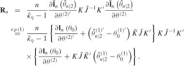
Proof of Proposition 8.3
The first result is an immediate consequence of Slutsky’s lemma and of the fact that under H0,
To show (8.23) in the standard case where θ0 ![]()
![]() , the asymptotic
, the asymptotic ![]() distribution is established by showing that Rn – Wn = oP(1). This equation does not hold true in our testing problem H0 : θ = θ0, where θ0 is on the boundary of Θ. Moreover, the asymptotic distribution of Wn is not
distribution is established by showing that Rn – Wn = oP(1). This equation does not hold true in our testing problem H0 : θ = θ0, where θ0 is on the boundary of Θ. Moreover, the asymptotic distribution of Wn is not ![]() - A more direct proof is thus necessary.
- A more direct proof is thus necessary.
Since ![]() is a consistent estimator of
is a consistent estimator of ![]() , > 0, we have, for n large enough,
, > 0, we have, for n large enough, ![]() > 0 and
> 0 and
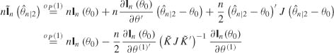
Let
Since
a Taylor expansion shows that
where ![]() means a = b + c. The last d2 components of this vectorial relation yield
means a = b + c. The last d2 components of this vectorial relation yield
and the first d1 components yield
using
We thus have
Using successively (8.40), (8.42) and (8.43), we obtain
Let
where W1 and W2 are vectors of respective sizes d1 and d2, and J11 is of size d1 × d1. Thus
where the last equality comes from Exercise 6.7. Using (8.44), the asymptotic distribution of Rn is thus that of
which follows a ![]() because it is easy to check that
because it is easy to check that
We have thus shown (8.23).
Now we show (8.24). Using (8.43) and (8.44), several Taylor expansions yield
and
By subtraction,
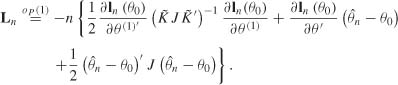
It can be checked that
Thus, the asymptotic distribution of Ln is that of
Moreover, it can easily be verified that
It follows that
which gives the first equality of (8.24). The second equality follows using Exercise 8.2. ![]()
Proof of Proposition 8.4
Since Cov(vt, ![]() ), we have
), we have
and the result follows from ![]() (see Proposition 2.2).
(see Proposition 2.2). ![]()
We first study the asymptotic impact of the unknown Initial values on the statistic ![]() m. Introduce the vector rm = (r(l), …, r(m))′, where
m. Introduce the vector rm = (r(l), …, r(m))′, where
Let st(θ) (![]() t(θ)) be the random variable obtained by replacing ηt by ηt(θ) =
t(θ)) be the random variable obtained by replacing ηt by ηt(θ) = ![]() t/σt(θ) (
t/σt(θ) (![]() t(θ) =
t(θ) = ![]() t/
t/![]() t(θ)) in st.The vectors rm(θ) and
t(θ)) in st.The vectors rm(θ) and ![]() m(θ) are defined similarly, so that rm = rm(θ0) and
m(θ) are defined similarly, so that rm = rm(θ0) and ![]() m =
m = ![]() m(
m(![]() n). Write
n). Write ![]() when a = b + c. Using (7.30) and the arguments used to show (d) on page 160, it can be shown that, as n → ∞,
when a = b + c. Using (7.30) and the arguments used to show (d) on page 160, it can be shown that, as n → ∞,
We now show that the asymptotic distribution of ![]()
![]() m is a function of the joint asymptotic distribution of
m is a function of the joint asymptotic distribution of ![]() rm and of the QMLE. By the arguments used to show (c) on page 160, it can be shown that there exists a neighborhood
rm and of the QMLE. By the arguments used to show (c) on page 160, it can be shown that there exists a neighborhood ![]() (θ0) of θ0 such that
(θ0) of θ0 such that
Using (8.45) and the fact that ![]() (
(![]() n − θ0), a Taylor expansion of rm(·) around
n − θ0), a Taylor expansion of rm(·) around ![]() n and θ0 shows that
n and θ0 shows that

for some θ* between ![]() n and θ0. Using (8.46), the ergodic theorem, the strong consistency of the QMLE, and a second Taylor expansion, we obtain
n and θ0. Using (8.46), the ergodic theorem, the strong consistency of the QMLE, and a second Taylor expansion, we obtain
where
For the next to last equality, we use the fact that ![]() . It follows that
. It follows that
We now derive the asymptotic distribution of ![]() (rm,
(rm, ![]() n − θ0). In the proof of Theorem 7.2, it is shown that
n − θ0). In the proof of Theorem 7.2, it is shown that
Note that ![]() where st − 1: t−m = (st−1, …, st−m)′- In view of (8.48), the central limit theorem applied to the martingale difference
where st − 1: t−m = (st−1, …, st−m)′- In view of (8.48), the central limit theorem applied to the martingale difference ![]() shows that
shows that
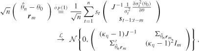
where
Using (8.47) and (8.49) together, we obtain
We now show that D is invertible. Because the law of ![]() is nondegenerate, we have κη>1. We thus have to show the invertibility of
is nondegenerate, we have κη>1. We thus have to show the invertibility of
If the previous matrix is singular then there exists λ = (λ1, …, λm)′ such that λ ≠ 0 and
with μ = λ′CmJ−1. Note that μ = (μ1, …, μp+ q + 1)′ ≠ 0. Otherwise λ′s−1:m = 0 a.s., which implies that there exists j ![]() {1, …, m} such that s−j is measurable with respect to σ{st, t ≠ − j}. This is impossible because the st are independent and nondegenerate by assumption A3 on page 144 (see Exercise 11.3). Denoting by Rt any random variable measurable with respect to σ{ηu, u ≤ t}, we have
{1, …, m} such that s−j is measurable with respect to σ{st, t ≠ − j}. This is impossible because the st are independent and nondegenerate by assumption A3 on page 144 (see Exercise 11.3). Denoting by Rt any random variable measurable with respect to σ{ηu, u ≤ t}, we have
and
Thus (8.50) entails that
Solving this quadratic equation in ![]() shows that either
shows that either ![]() which is impossible by arguments already given, or λ1α1 = 0. Let λ′2:m = (λ2, …, λm)′. If λ1 = 0 then (8.50) implies that
which is impossible by arguments already given, or λ1α1 = 0. Let λ′2:m = (λ2, …, λm)′. If λ1 = 0 then (8.50) implies that
Taking the expectation with respect to σ{ηt, t ≤ −2}, it can be seen that ![]() in the previous equality. Thus we have
in the previous equality. Thus we have
which entails α1 = μ2 = 0, because P {(λ2,…, λm)′s−2:−m = 0} < 1 (see Exercise 8.12). For GARCH (p, 1) models, it is impossible to have α1 = 0 by assumption A4. The invertibility of D is thus shown in this case. In the general case, we show by induction that (8.50) entails α1 = … αp.
It is easy to show that ![]() → D in probability (and even almost surely) as n → ∞. The conclusion follows.
→ D in probability (and even almost surely) as n → ∞. The conclusion follows. ![]()
It is well known that when the parameter is at the boundary of the parameter space, the maximum likelihood estimator does not necessarily satisfy the first-order conditions and, in general, does not admit a limiting normal distribution. The technique, employed in particular by Chernoff (1954) and Andrews (1997) in a general framework, involves approximating the quasi-likelihood by a quadratic function, and defining the asymptotic distribution of the QML as that of the projection of a Gaussian vector on a convex cone. Particular GARCH models are considered by Andrews (1997, 1999) and Jordan (2003). The general GARCH(p, q) case is considered by Francq and Zakoïan (2007). A proof of Theorem 8.1, when the moment assumption B7 is replaced by assumption B7′ of Remark 8.2, can be found in the latter reference. When the nullity of GARCH coefficients is tested, the parameter is at the boundary of the parameter space under the null, and the alternative is one-sided. Numerous works deal with testing problems where, under the null hypothesis, the parameter is at the boundary of the parameter space. Such problems have been considered by Chernoff (1954), Bartholomew (1959), Perlman (1969) and Gouriéroux, Holly and Monfort (1982), among many others. General one-sided tests have been studied by, for instance, Rogers (1986), Wolak (1989), Silvapulle and Silvapulle (1995) and King and Wu (1997). Papers dealing more specifically with ARCH and GARCH models are Lee and King (1993), Hong (1997), Demos and Sentana (1998), Andrews (2001), Hong and Lee (2001), Dufour et al. (2004) and Francq and Zakoïan (2009b).
The portmanteau tests based on the squared residual autocovariances were proposed by McLeod and Li (1983), Li and Mak (1994) and Ling and Li (1997). The results presented here closely follow Berkes, Horváth and Kokoszka (2003a). Problems of interest that are not studied in this book are the tests on the distribution of the iid process (see Horváth, Kokoszka and Teyssiére, 2004; Horváth and Zitikis, 2006).
Concerning the overrepresentation of the GARCH(1, 1) model in financial studies, we mention Stărică (2006). This paper highlights, on a very long S&P 500 series, the poor performance of the GARCH(1, 1) in terms of prediction and modeling, and suggests a nonstationary dynamics of the returns.
8.1 (Minimization of a distance under a linear constraint)
Let J be an n × n invertible matrix, let x0 be a vector of ![]() n, and let K be a full-rank p × n matrix, p ≤ n. Solve the problem of the minimization of Q(x) = (x − x0)′J(x − x0) under the constraint Kx = 0.
n, and let K be a full-rank p × n matrix, p ≤ n. Solve the problem of the minimization of Q(x) = (x − x0)′J(x − x0) under the constraint Kx = 0.
8.2 (Minimization of a distance when some components are equal to zero)
Let J be an n × n invertible matrix, x0 a vector of ![]() n and p < n. Minimize Q(x) = (x −0 x0) J(x − x0) under the constraints
n and p < n. Minimize Q(x) = (x −0 x0) J(x − x0) under the constraints ![]() (xi denoting the ith component of x, and assuming that 1 ≤ i1 < … < ip ≤ n).
(xi denoting the ith component of x, and assuming that 1 ≤ i1 < … < ip ≤ n).
8.3 (Lagrangian or method of substitution for optimization with constraints)
Compare the solutions (C.13) and (C.14) of the optimization problem of Exercise 8.2, with
and the constraints
(a) x3 = 0,
(b) x2 = x3 = 0.
8.4 (Minimization of a distance under inequality constraints)
Find the minimum of the function
under the constraints λ2 ≥ 0 and λ2 ≥ 0, when
(i) Z = (−2,l,2)′,
(ii) Z = (−2,−1,2)′,
(iii) Z = (−2, 1, −2)′,
(iv) Z = (−2,−1,-2)′.
8.5 (Influence of the positivity constraints on the moments of the QMLE)
Compute the mean and variance of the vector λι defined by (8.16). Compare these moments with the corresponding moments of Z = (Z1, Z2, Z3)′.
8.6 (Asymptotic distribution of the QMLE of an ARCH in the conditionally homoscedastic case)
For an ARCH(q) model, compute the matrix Σ involved in the asymptotic distribution of the QMLE in the case where all the α0i are equal to zero.
8.7 (Asymptotic distribution of the QMLE when an ARCH (1) is fitted to a strong white noise)
Let ![]() be the QMLE in the ARCH(l) model
be the QMLE in the ARCH(l) model ![]() when the true parameter is equal to (ω0,α0) = (ω0, 0) and when
when the true parameter is equal to (ω0,α0) = (ω0, 0) and when ![]() . Give an expression for the asymptotic distribution of
. Give an expression for the asymptotic distribution of ![]() (
(![]() − θ0) with the aid of
− θ0) with the aid of
Compute the mean vector and the variance matrix of this asymptotic distribution. Determine the density of the asymptotic distribution of ![]() (
(![]() − ω0). Give an expression for the kurtosis coefficient of this distribution as function of κη.
− ω0). Give an expression for the kurtosis coefficient of this distribution as function of κη.
8.8 (One-sided and two-sided tests have the same Bahadur slopes)
Let X1, …, Xn be a sample from the ![]() (θ, 1) distribution. Consider the null hypothesis H0 : θ = 0. Denote by Φ the F10D;(0, 1) cumulative distribution function. By the Neyman–Pearson lemma, we know that, for alternatives of the form H1 : θ > 0, the one-sided test of rejection region
(θ, 1) distribution. Consider the null hypothesis H0 : θ = 0. Denote by Φ the F10D;(0, 1) cumulative distribution function. By the Neyman–Pearson lemma, we know that, for alternatives of the form H1 : θ > 0, the one-sided test of rejection region
is uniformly more powerful than the two-sided test of rejection region
(moreover, C is uniformly more powerful than any other test of level α or less). Although we just have seen that the test C is superior to the test C* in finite samples, we will conduct an asymptotic comparison of the two tests, using the Bahadur and Pitman approaches.
• The asymptotic Bahadur slope c(θ) is defined as the almost sure limit of − 2/n times the logarithm of the p-value under Pθ, when the limit exists. Compare the Bahadur slopes of the two tests.
• In the Pitman approach, we define a local power around θ = 0 as being the power at τ/![]() . Compare the local powers of C and C*. Compare also the local asymptotic powers of the two tests for non-Gaussian samples.
. Compare the local powers of C and C*. Compare also the local asymptotic powers of the two tests for non-Gaussian samples.
8.9 (The local asymptotic approach cannot distinguish the Wald, score and likelihood ratio tests)
Let X1, …, Xn be a sample of the ![]() (θ, τ2) distribution, where θ and τ2 are unknown. Consider the null hypothesis H0 : θ = 0 against the alternative H1 : θ > 0. Consider the following three tests:
(θ, τ2) distribution, where θ and τ2 are unknown. Consider the null hypothesis H0 : θ = 0 against the alternative H1 : θ > 0. Consider the following three tests:
• ![]() , where
, where
is the Wald statistic;
• ![]() . where
. where
is the Rao score statistic;
• ![]() , where
, where
is the likelihood ratio statistic.
Give a justification for these three tests. Compare their local asymptotic powers and their Bahadur slopes.
8.10 (The Wald and likelihood ratio statistics have the same asymptotic distribution)
Consider the case d2 = 1, that is, the framework of Section 8.3.3 where only one coefficient is equal to zero. Without using Remark 8.3, show that the asymptotic laws W and L defined by (8.22) and (8.24) are such that
8.11 (For testing conditional homoscedasticity, the Wald and likelihood ratio statistics have the same asymptotic distribution)
Repeat Exercise 8.10 for the conditional homoscedasticity test (8.26) in the ARCH(q) case.
8.12 (The product of two independent random variables is null if and only if one of the two variables is null)
Let X and Y be two independent random variables such that XY = 0 almost surely. Show that either X = 0 almost surely or Y = 0 almost surely.
1 The term ‘approximate’ is used by Bahadur (1960) to emphasize that the exact survival function ![]() (t) is approximated by the asymptotic survival function SW (t). See also Bahadur (1967) for a discussion on the exact and approximate slopes.
(t) is approximated by the asymptotic survival function SW (t). See also Bahadur (1967) for a discussion on the exact and approximate slopes.