Identification
In this chapter, we consider the problem of selecting an appropriate GARCH or ARMA-GARCH model for given observations X1, …, Xn of a centered stationary process. A large part of the theory of finance rests on the assumption that prices follow a random walk. The price variation process, X = (Xt), should thus constitute a martingale difference sequence, and should coincide with its innovation process, ![]() = (
= (![]() t). The first question addressed in this chapter, in Section 5.1, will be the test of this property, at least a consequence of it: absence of correlation. The problem is far from trivial because standard tests for noncorrelation are actually valid under an independence assumption. Such an assumption is too strong for GARCH processes which are dependent though uncorrelated.
t). The first question addressed in this chapter, in Section 5.1, will be the test of this property, at least a consequence of it: absence of correlation. The problem is far from trivial because standard tests for noncorrelation are actually valid under an independence assumption. Such an assumption is too strong for GARCH processes which are dependent though uncorrelated.
If significant sample autocorrelations are detected in the price variations - in other words, if the random walk assumption cannot be sustained - the practitioner will try to fit an ARMA(P, Q) model to the data before using a GARCH(p, q) model for the residuals. Identification of the orders (P, Q) will be treated in Section 5.2, identification of the orders (p,q) in Section 5.3. Tests of the ARCH effect (and, more generally, Lagrange multiplier tests) will be considered in Section 5.4.
5.1 Autocorrelation Check for White Noise
Consider the GARCH(p, q) model
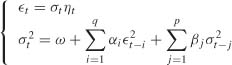
with (ηt) a sequence of iid centered variables with unit variance, ω > 0, αi ≥ 0 (i = 1, …, q), βj ≥ 0 (j = 1, …, p). We saw in Section 2.2 that, whatever the orders p and q, the nonanticipative second-order stationary solution of (5.1) is a white noise, that is, a centered process whose theoretical autocorrelations ρ(h) = E![]() t
t![]() t + h/E
t + h/E![]() satisfy ρ(h) = 0 for all h ≠ 0.
satisfy ρ(h) = 0 for all h ≠ 0.
Given observations ![]() 1, …, …n, the theoretical autocorrelations of a centered process (
1, …, …n, the theoretical autocorrelations of a centered process (![]() t) are generally estimated by the sample autocorrelations (SACRs)
t) are generally estimated by the sample autocorrelations (SACRs)
for h = 0, 1, …, n − 1. According to Theorem 1.1, if (![]() t) is an iid sequence of centered random variables with finite variance then
t) is an iid sequence of centered random variables with finite variance then
for all h ≠ 0. For a strong white noise, the SACRs thus lie between the confidence bounds ±1.96/![]() with a probability of approximately 95% when n is large. In standard software, these bounds at the 5% level are generally displayed with dotted lines, as in Figure 5.2. These significance bands are not valid for a weak white noise, in particular for a GARCH process (Exercises 5.3 and 5.4). Valid asymptotic bands are derived in the next section.
with a probability of approximately 95% when n is large. In standard software, these bounds at the 5% level are generally displayed with dotted lines, as in Figure 5.2. These significance bands are not valid for a weak white noise, in particular for a GARCH process (Exercises 5.3 and 5.4). Valid asymptotic bands are derived in the next section.
5.1.1 Behavior of the Sample Autocorrelations of a GARCH Process
Let ![]() m = (
m = (![]() (1),...,
(1),...,![]() (m))′ denote the vector of the first m SACRs, based on n observations of the GARCH(p, q) process defined by (5.1). Let
(m))′ denote the vector of the first m SACRs, based on n observations of the GARCH(p, q) process defined by (5.1). Let ![]() m = (
m = (![]() (1),...,
(1),...,![]() (m))′ denote a vector of sample autocovariances (SACVs).
(m))′ denote a vector of sample autocovariances (SACVs).
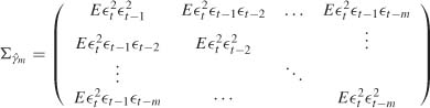
Theorem 5.1 (Asymptotic distributions of the SACYs and SACRs) If (![]() t) is the nonanticipative and stationary solution of the GARCH(p, q) model (5.1) and if E
t) is the nonanticipative and stationary solution of the GARCH(p, q) model (5.1) and if E![]() < ∞, then, when n → ∞,
< ∞, then, when n → ∞,
where
is nonsingular. If the law of ηt is symmetric then ![]()
![]() m is diagonal.
m is diagonal.
Note that ![]()
![]() m when (
m when (![]() t) is a strong white noise, in accordance with Theorem 1.1.
t) is a strong white noise, in accordance with Theorem 1.1.
Proof. Let ![]() m = (
m = (![]() (1),...,
(1),...,![]() (m))′, where
(m))′, where ![]() . Since, for m fixed,
. Since, for m fixed,
as n → ∞, the asymptotic distribution of ![]()
![]() m coincides with that of
m coincides with that of ![]()
![]() m. Let h and k belong to {1, …, m}. By stationarity,
m. Let h and k belong to {1, …, m}. By stationarity,
because
From this, we deduce the expression for ![]()
![]() m. From the Cramér-Wold theorem,1 the asymptotic normality of
m. From the Cramér-Wold theorem,1 the asymptotic normality of ![]()
![]() m will follow from showing that for all nonzero λ = (λ1, …, λm)′
m will follow from showing that for all nonzero λ = (λ1, …, λm)′ ![]()
![]() m,
m,
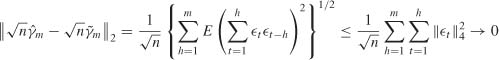
Let Ft denote the σ-field generated by {![]() u, u ≤ t}. We obtain (5.3) by applying a central limit theorem (CLT) to the sequence
u, u ≤ t}. We obtain (5.3) by applying a central limit theorem (CLT) to the sequence ![]() , which is a stationary, ergodic and square integrable martingale difference (see Corollary A.l).
, which is a stationary, ergodic and square integrable martingale difference (see Corollary A.l).
The asymptotic behavior of ![]() m immediately follows from that of
m immediately follows from that of ![]() m(as in Exercise 5.3).
m(as in Exercise 5.3).
Reasoning by contradiction, suppose that ![]()
![]() m is singular. Then, because this matrix is the covariance of the vector (
m is singular. Then, because this matrix is the covariance of the vector (![]() t
t![]() t − 1, …,
t − 1, …, ![]() t
t![]() t − m)′, there exists an exact linear combination of the components of (
t − m)′, there exists an exact linear combination of the components of (![]() t
t![]() t − 1, …,
t − 1, …, ![]() t
t![]() t − m)′ that is equal to zero. For some i0 ≥ 1, we then have
t − m)′ that is equal to zero. For some i0 ≥ 1, we then have ![]() , that is,
, that is, ![]() . Hence,
. Hence,
which is absurd. It follows that ![]()
![]() m is nonsingular.
m is nonsingular.
When the law of ηt is symmetric, the diagonal form of ![]()
![]() m is a consequence of property (7.24) in Chapter 7. See Exercises 5.5 and 5.6 for the GARCH(1, 1) case.
m is a consequence of property (7.24) in Chapter 7. See Exercises 5.5 and 5.6 for the GARCH(1, 1) case. ![]()
A consistent estimator ![]()
![]() m of
m of ![]()
![]() m is obtained by replacing the generic term of
m is obtained by replacing the generic term of ![]()
![]() m by
m by
with, by convention, ![]() s=0 for s < 1. Clearly,
s=0 for s < 1. Clearly, ![]() is a consistent estimator of
is a consistent estimator of ![]()
![]() m and is almost surely invertible for n large enough. This can be used to construct asymptotic significance bands for the SACRs of a GARCH process.
m and is almost surely invertible for n large enough. This can be used to construct asymptotic significance bands for the SACRs of a GARCH process.
The following R code allows us to draw a given number of autocorrelations ![]() (i); and the significance bands
(i); and the significance bands ![]() .
.
# autocorrelation function
gamma<-function(x, h){ n<-length(x); h<-abs(h);x<-x-mean(x)
+ gamma<-sum(x[1:(n-h)]*x[(h+1):n])/n }
rho<-function(x,h) rho<-gamma(x,h)/gamma(x,0)
# acf function with significance bands of a strong white noise
nl.acf<-function(x,main=NULL,method=‘NP’){
+ n<-length(x); nlag<-as.integer(min(10*logl0(n),n−l)) +
acf.val<-sapply(c(1:nlag),function(h) rho(x,h)) + x2<-x^2 +
var<-l+(sapply(c(1:nlag),function(h) gamma(x2,h)))/gamma(x,0)^2 +
band<-sqrt(var/n) +
minval<-l.2*min(acf.val, −1.96*band,−1.96/sqrt(n)) +
maxval<-l.2*max(acf.val,1.96*band,1.96/sqrt(n)) +
acf(x,xlab=‘Lag’,ylab=‘SACR’, ylim^c(minval,maxval)/main=main) +
lines(c(1:nlag),−1.96*band,lty=l,col=‘red’) +
lines(c(l:nlag),1.96*band,lty=l,col=‘red’)}
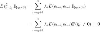
In Figure 5.1 we have plotted the SACRs and their significance bands for daily series of exchange rates of the dollar, pound, yen and Swiss franc against the euro, for the period from January 4, 1999 to January 22, 2009. It can be seen that the SACRs are often outside the standard significance bands ±1.96/![]() , which leads us to reject the strong white noise assumption for all these series. On the other hand, most of the SACRs are inside the significance bands shown as solid lines, which is in accordance with the hypothesis that the series are realizations of semi-strong white noises.
, which leads us to reject the strong white noise assumption for all these series. On the other hand, most of the SACRs are inside the significance bands shown as solid lines, which is in accordance with the hypothesis that the series are realizations of semi-strong white noises.
Figure 5.1 SACR of exchange rates against the euro, standard significance bands for the SACRs of a strong white noise (dotted lines) and significance bands for the SACRs of a semi-strong white noise (solid lines).
The standard portmanteau test for checking that the data is a realization of a strong white noise is that of Ljung and Box (1978). It involves computing the statistic
and rejecting the strong white noise hypothesis if ![]() is greater than the (1 − α)-quantile of a
is greater than the (1 − α)-quantile of a ![]() 2
2
Portmanteau tests are constructed for checking noncorrelation, but the asymptotic distribution of the statistics is no longer ![]() when the series departs from the strong white noise assumption. For instance, these tests are not robust to conditional heteroscedasticity. In the GARCH framework, we may wish to simultaneously test the nullity of the first m autocorrelations using more robust portmanteau statistics.
when the series departs from the strong white noise assumption. For instance, these tests are not robust to conditional heteroscedasticity. In the GARCH framework, we may wish to simultaneously test the nullity of the first m autocorrelations using more robust portmanteau statistics.
Theorem 5,2 (Corrected portmanteau test in the presence of ARCH) Under the assumptions of Theorem 5.1, the portmanteau statistic
has an asymptotic ![]() distribution.
distribution.
Proof. Ii suffices to use Theorem 5.1 and the following result: if ![]() , with Σ nonsingular, and if in probability, then
, with Σ nonsingular, and if in probability, then ![]() .
. ![]()
A portmanteau test of asymptotic level α based on the first m SACRs involves rejecting the hypothesis that the data are generated by a GARCH process if Qm is greater than the (1 − α)-quantile of a ![]() .
.
5.1.3 Sample Partial Autocorrelations of a GARCH
Denote by rm(![]() m) the vector of the m first partial autocorrelations (sample partial autocorrelations (SPACs)) of the process (
m) the vector of the m first partial autocorrelations (sample partial autocorrelations (SPACs)) of the process (![]() t). By Theorem B.3, we know that for a weak white noise, the SACRs and SPACs have the same asymptotic distribution. This applies in particular to a GARCH process. Consequently, under the hypothesis of GARCH white noise with a finite fourth-order moment, consistent estimators of
t). By Theorem B.3, we know that for a weak white noise, the SACRs and SPACs have the same asymptotic distribution. This applies in particular to a GARCH process. Consequently, under the hypothesis of GARCH white noise with a finite fourth-order moment, consistent estimators of ![]()
![]() m are
m are
where ![]() m is the matrix obtained by replacing ρx(1), …, ρx(m) by , …, in the Jacobian matrix Jm of the mapping , and is the consistent estimator of
m is the matrix obtained by replacing ρx(1), …, ρx(m) by , …, in the Jacobian matrix Jm of the mapping , and is the consistent estimator of ![]()
![]() m defined after Theorem 5.1.
m defined after Theorem 5.1.
Although it is not current practice, one can test the simultaneous nullity of several theoretical partial autocorrelations using portmanteau tests based on the statistics
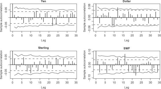
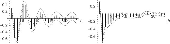
Figure 5.2 SACRs of a simulation of a strong white noise (left) and of the GARCH(1, 1) white noise (5.4) (right). Approximately 95% of the SACRs of a strong white noise should lie inside the thin dotted lines ±1.96/![]() . Approximately 95% of the SACRs of a GARCH(1, 1) white noise should lie inside the thick dotted lines.
. Approximately 95% of the SACRs of a GARCH(1, 1) white noise should lie inside the thick dotted lines.
with, for instance, i = 2. From Theorem B.3, under the strong white noise assumption, the statistics ![]() and
and ![]() have the same
have the same ![]() asymptotic distribution. Under the hypothesis of a pure GARCH process, the statistics
asymptotic distribution. Under the hypothesis of a pure GARCH process, the statistics ![]() and Qm also have the same
and Qm also have the same ![]() asymptotic distribution.
asymptotic distribution.
Standard Significance Bounds for the SACRs are not Valid
The right-hand graph of Figure 5.2 displays the sample correlogram of a simulation of size n = 5000 of the GARCH(1, 1) white noise
where (ηt) is a sequence of iid N (0, 1) variables. It is seen that the SACRs of order 2 and 4 are sharply outside the 95% significance bands computed under the strong white noise assumption. An inexperienced practitioner could be tempted to reject the hypothesis of white noise, in favor of a more complicated ARMA model whose residual autocorrelations would lie between the significance bounds ±1.96/![]() . To avoid this type of specification error, one has to be conscious that the bounds ±1.96/
. To avoid this type of specification error, one has to be conscious that the bounds ±1.96/![]() are not valid for the SACRs of a GARCH white noise. In our simulation, it is possible to compute exact asymptotic bounds at the 95% level (Exercise 5.4). In the right-hand graph of Figure 5.2, these bounds are drawn in thick dotted lines. All the SACRs are now inside, or very slightly outside, those bounds. If we had been given the data, with no prior information, this graph would have given us no grounds on which to reject the simple hypothesis that the data is a realization of a GARCH white noise.
are not valid for the SACRs of a GARCH white noise. In our simulation, it is possible to compute exact asymptotic bounds at the 95% level (Exercise 5.4). In the right-hand graph of Figure 5.2, these bounds are drawn in thick dotted lines. All the SACRs are now inside, or very slightly outside, those bounds. If we had been given the data, with no prior information, this graph would have given us no grounds on which to reject the simple hypothesis that the data is a realization of a GARCH white noise.
Estimating the Significance Bounds of the SACRs of a GARCH
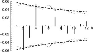
Of course, in real situations the significance bounds depend on unknown parameters, and thus cannot be easily obtained. It is, however, possible to estimate them in a consistent way, as described in Section 5.1.1. For a simulation of model (5.4) of size n = 5000, Figure 5.3 shows as thin dotted lines the estimation thus obtained of the significance bounds at the 5% level. The estimated bounds are fairly close to the exact asymptotic bounds.
The SPACs and Their Significance Bounds
Figure 5.4 shows the SPACs of the simulation (5.4) and the estimated significance bounds of the ![]() (h), at the 5% level (based on
(h), at the 5% level (based on ![]() ). By comparing Figures 5.3 and 5.4, it can be seen that the
). By comparing Figures 5.3 and 5.4, it can be seen that the
Figure 5.3 Sample autocorrelations of a simulation of size n = 5000 of the GARCH(1, 1) white noise (5.4). Approximately 95% of the SACRs of a GARCH(1, 1) white noise should lie inside the thin dotted lines. The exact asymptotic bounds are shown as thick dotted lines.
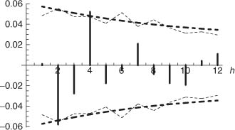
Figure 5.4 Sample partial autocorrelations of a simulation of size n = 5000 of the GARCH(1, 1) white noise (5.4). Approximately 95% of the SPACs of a GARCH(1, 1) white noise should lie inside the thin dotted lines. The exact asymptotic bounds are shown as thick dotted lines.
SACRs and SPACs of the GARCH simulation look much alike. This is not surprising in view of Theorem B.4.
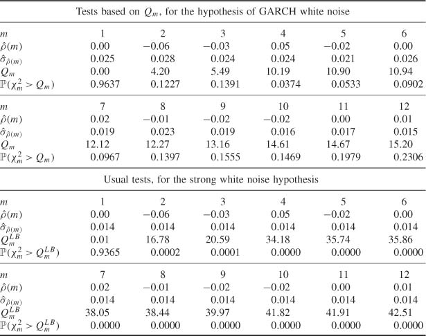
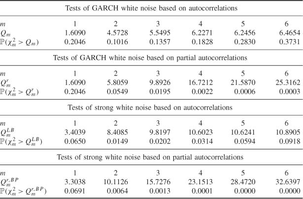
Portmanteau Tests of Strong White Noise and of Pure GARCH
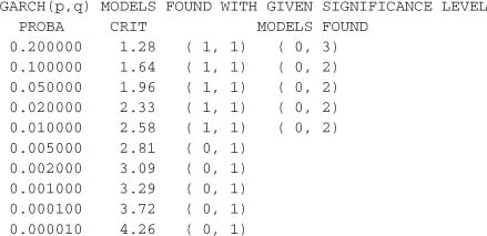
Table 5.1 displays p-values of white noise tests based on Qm and the usual Ljung-Box statistics, for the simulation of (5.4). Apart from the test with m = 4, the Qm tests do not reject, at the 5% level, the hypothesis that the data comes from a GARCH process. On the other hand, the Ljung-Box tests clearly reject the strong white noise assumption.
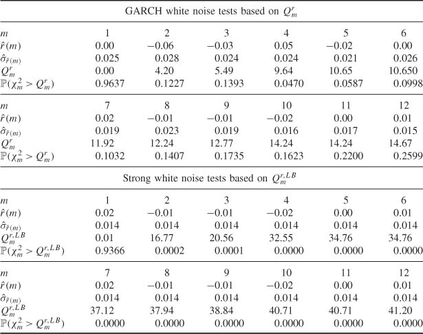
Portmanteau Tests Based on Partial Autocorrelations
Table 5.2 Is similar to Table 5.1, but presents portmanteau tests based on the SPACs. As expected, the results are very close to those obtained for the SACRs.
An Example Showing that Portmanteau Tests Based on the SPACs Can Be More Powerful than those Based on the SACRs
Consider a simulation of size n = 100 of the strong MA(2) model
By comparing the top two and bottom two parts of Table 5.3, we note that the hypotheses of strong white noise and pure GARCH are better rejected when the SPACs, rather than the SACRs, are used. This follows from the fact that, for this MA(2), only two theoretical autocorrelations are not equal to 0, whereas many theoretical partial autocorrelations are far from 0. For the same reason, the results would have been inverted if, for instance, an AR(1) alternative had been considered.
5.2 Identifying the ARMA Orders of an ARMA-GARCH
Assume that the tools developed in Section 5.1 lead to rejection of the hypothesis that the data is a realization of a pure GARCH process. It is then sensible to look for an ARMA(P, Q) model with GARCH innovations. The problem is then to choose (or identify) plausible orders for the model
under standard assumptions (the AR and MA polynomials having no common root and having roots outside the unit disk, with ![]() ), where (
), where (![]() t) is a GARCH white noise of the form (5.1).
t) is a GARCH white noise of the form (5.1).
5.2.1 Sample Autocorrelations of an ARMA-GARCH
Recall that an MA(Q) satisfies ρx(h) = 0 for all h > Q, whereas an AR(P) satisfies rx(h) = 0 for all h > P. The SACRs and SPACs thus play an important role in identifying the orders P and Q.
Invalidity of the Standard Bartlett Formula and Modified Formula
The validity of the usual Bartlett formula rests on assumptions including the strong white noise hypothesis (Theorem 1.1) which are obviously incompatible with GARCH errors. We shall see that this formula leads to underestimation of the variances of the SACRs and SPACs, and thus to erroneous ARMA orders. We shall only consider the SACRs because Theorem B.2 shows that the asymptotic behavior of the SPACs easily follows from that of the SACRs.
We assume throughout that the law of ηt is symmetric. By Theorem B.5, the asymptotic behavior of the SACRs is determined by the generalized Bartlett formula (B.15). This formula involves the theoretical autocorrelations of (Xt) and (![]() ), as well as the ratio
), as well as the ratio ![]() . More precisely, using Remark 1 of Theorem 7.2.2 in Brockwell and Davis (1991), the generalized Bartlett formula is written as
. More precisely, using Remark 1 of Theorem 7.2.2 in Brockwell and Davis (1991), the generalized Bartlett formula is written as
where
and
The following result shows that the standard Bartlett formula always underestimates the asymptotic variances of the sample autocorrelations in presence of GARCH errors.
Proposition 5.1 Under the assumptions of Theorem B.5, if the linear innovation process (![]() t) is a GARCH process with ηt symmetrically distributed, then
t) is a GARCH process with ηt symmetrically distributed, then
If moreover, α1 > 0, Var(![]() )> 0 and
)> 0 and ![]() , then
, then
Proof. From Proposition 2.2, we have ![]() for all
for all ![]() , with strict inequality when α1 > 0. It thus follows immediately from (5.7) that
, with strict inequality when α1 > 0. It thus follows immediately from (5.7) that ![]() . When α1 > 0 this inequality is strict unless if κ
. When α1 > 0 this inequality is strict unless if κ![]() = 1 or wi(
= 1 or wi(![]() ) = 0 for all
) = 0 for all ![]() ≥ 1, that is,
≥ 1, that is,
Suppose this relations holds and note that it is also satisfied for all ![]()
![]()
![]() . Moreover, summing over
. Moreover, summing over ![]() , we obtain
, we obtain
Because the sum of all autocorrelations is supposed to be nonzero, we thus have ρx(i) = 1. Taking ![]() = i in the previous relation, we thus find that ρx(2i) = 1. Iterating this argument yields ρx(ni) = 1, and letting n go to infinity gives a contradiction. Finally, one cannot have κ
= i in the previous relation, we thus find that ρx(2i) = 1. Iterating this argument yields ρx(ni) = 1, and letting n go to infinity gives a contradiction. Finally, one cannot have κ![]() = 1 because
= 1 because
Consider, by way of illustration, the ARMA(2,1)-GARCH(1, 1) process defined by
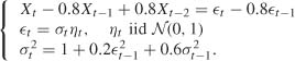
Figure 5.5 shows the theoretical autocorrelations and partial autocorrelations for this model. The bands shown as solid lines should contain approximately 95% of the SACRs and SPACs, for a realization of size n = 1000 of this model. These bands are obtained from formula (B.15), the autocorrelations of (![]() ) being computed as in Section 2.5.3. The bands shown as dotted lines correspond to the standard Bartlett formula (still at the 95% level). It can be seen that using this formula, which is erroneous in the presence of GARCH, would lead to identification errors because it systematically underestimates the variability of the sample autocorrelations (Proposition 5.1).
) being computed as in Section 2.5.3. The bands shown as dotted lines correspond to the standard Bartlett formula (still at the 95% level). It can be seen that using this formula, which is erroneous in the presence of GARCH, would lead to identification errors because it systematically underestimates the variability of the sample autocorrelations (Proposition 5.1).
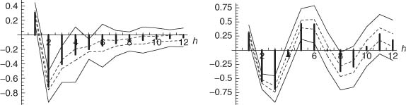
Algorithm for Estimating the Generalized Bands
In practice, the autocorrelations of (Xt) and (![]() ), as well as the other theoretical quantities involved in the generalized Bartlett formula (B.15), are obviously unknown. We propose the following algorithm for estimating such quantities:
), as well as the other theoretical quantities involved in the generalized Bartlett formula (B.15), are obviously unknown. We propose the following algorithm for estimating such quantities:
1. Fit an AR(p0) model to the data X1, …, Xn using an information criterion for the selection of the order p0.
2. Compute the autocorrelations ρ1(h), h = 1, 2, –, of this AR(p0) model.
3. Compute the residuals ep0 + 1, …, en of this estimated AR(p0).
4. Fit an AR(p1) model to the squared residuals ![]() , again using an information criterion for p1.
, again using an information criterion for p1.
Figure 5.5 Autocorrelations (left) and partial autocorrelations (right) for model (5.8). Approximately 95% of the SACRs (SPACs) of a realization of size n = 1000 should lie between the bands shown as solid lines. The bands shown as dotted lines correspond to the standard Bartlett formula.
5. Compute the autocorrelations ρ2(h), h = 1, 2, …, of this AR(p1) model.
6. Estimate limn → ∞ nCov![]() by
by ![]() , where
, where
and ![]() max is a truncation parameter, numerically determined so as to have |ρ1(
max is a truncation parameter, numerically determined so as to have |ρ1(![]() )| and |ρ2(
)| and |ρ2(![]() )| less than a certain tolerance (for instance, 10−5) for all
)| less than a certain tolerance (for instance, 10−5) for all ![]() >
> ![]() max.
max.
This algorithm is fast when the Durbin-Levinson algorithm is used to fit the AR models. Figure 5.6 shows an application of this algorithm (using the BIC information criterion).
5.2.2 Sample Autocorrelations of an ARMA-GARCH Process When the Noise is Not Symmetrically Distributed
The generalized Bartlett formula (B.15) holds under condition (B.13), which may not be satisfied if the distribution of the noise ηt, in the GARCH equation, is not symmetric. We shall consider the asymptotic behavior of the SACVs and SACRs for very general linear processes whose innovation (![]() t) is a weak white noise. Retaining the notation of Theorem B.5, the following property allows the asymptotic variance of the SACRs to be interpreted as the spectral density at 0 of a vector process (see, for instance, Brockwell and Davis, 1991, for the concept of spectral density). Let
t) is a weak white noise. Retaining the notation of Theorem B.5, the following property allows the asymptotic variance of the SACRs to be interpreted as the spectral density at 0 of a vector process (see, for instance, Brockwell and Davis, 1991, for the concept of spectral density). Let ![]()
Theorem 5.3 Let (Xt)t![]()
![]() be a real stationary process satisfying
be a real stationary process satisfying
Figure 5.6 SACRs (left) and SPACs (right) of a simulation of size n = 1000 of model (5.8). The dotted lines are the estimated 95% confidence bands.
where (![]() t)t
t)t![]()
![]() is a weak white noise such that E
is a weak white noise such that E![]() <∞. Let Yt = Xt (Xt, Xt + 1, …, Xt + m)′,
<∞. Let Yt = Xt (Xt, Xt + 1, …, Xt + m)′, ![]() and
and ![]()
the spectral density of the process ![]() . Then we have
. Then we have
Proof. By stationarity and application of the Lebesgue dominated convergence theorem,
as n → ∞ ![]()
The matrix ![]() involved in (5.9) is called the long-run variance in the econometric literature, as a reminder that it is the limiting variance of a sample mean. Several methods can be considered for long-run variance estimation.
involved in (5.9) is called the long-run variance in the econometric literature, as a reminder that it is the limiting variance of a sample mean. Several methods can be considered for long-run variance estimation.
(i) The naive estimator based on replacing the ![]() Y(h) by the
Y(h) by the ![]() in fY*(0) is inconsistent (Exercise 1.2). However, a consistent estimator can be obtained by weighting the
in fY*(0) is inconsistent (Exercise 1.2). However, a consistent estimator can be obtained by weighting the ![]() , using a weight close to 1 when h is very small compared to n, and a weight close to 0 when h is large. Such an estimator is called heteroscedastic and autocorrelation consistent (HAC) in the econometric literature.
, using a weight close to 1 when h is very small compared to n, and a weight close to 0 when h is large. Such an estimator is called heteroscedastic and autocorrelation consistent (HAC) in the econometric literature.
(ii) A consistent estimator of fY*(0) can also be obtained using the smoothed periodogram (see Brockwell and Davis, 1991, Section 10.4).
(iii) For a vector AR(r),
the spectral density at 0 is
A vector AR model is easily fitted, even a high-order AR, using a multivariate version of the Durbin-Levinson algorithm (see Brockwell and Davis, 1991, p. 422). The following method can thus be proposed:
1. Fit AR(r) models, with r = 0, 1 …, R, to the data ![]() where
where ![]()
2. Select a value r0 by minimizing an information criterion, for instance the BIC.
with obvious notation.
In our applications we used method (iii).
5.2.3 Identifying the Orders (P, Q)
Order determination based on the sample autocorrelations and partial autocorrelations in the mixed ARMA(P, Q) model is not an easy task. Other methods, such as the corner method, presented in the next section, and the epsilon algorithm, rely on more convenient statistics.
The Corner Method
Denote by D(i, j) the j × j Toeplitz matrix
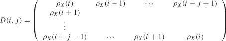
and let Δ(i, j) denote its determinant. Since ![]() , for all h > Q, it is clear that D(i, j) is not a full-rank matrix if i > Q and j > P. More precisely, P and Q are minimal orders (that is, (Xt) does not admit an ARMA(P′, Q′) representation with P′ < P or Q′ < Q) if and only if
, for all h > Q, it is clear that D(i, j) is not a full-rank matrix if i > Q and j > P. More precisely, P and Q are minimal orders (that is, (Xt) does not admit an ARMA(P′, Q′) representation with P′ < P or Q′ < Q) if and only if
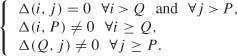
The minimal orders P and Q are thus characterized by the following table:
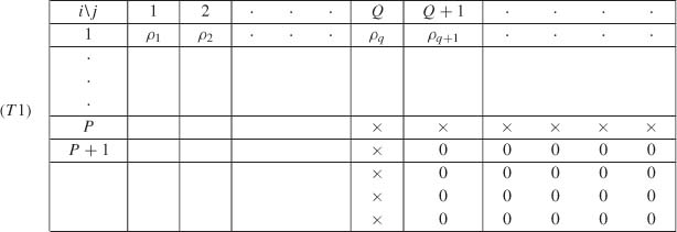
where Δ(j, i) is at the intersection of row i and column j, and × denotes a nonzero element.
The orders P and Q are thus characterized by a corner of zeros in table (T1), hence the term ‘corner method’. The entries in this table are easily obtained using the recursion on j given by
and letting Δ(i, 0) = 1, Δ(i, 1) = ρx(|i|).
Denote by ![]() , … the items obtained by replacing {ρx(h)} by
, … the items obtained by replacing {ρx(h)} by ![]() in D(i, j), Δ(i, j), (T1), …. Only a finite number of SACRs
in D(i, j), Δ(i, j), (T1), …. Only a finite number of SACRs ![]() are available in practice, which allows
are available in practice, which allows ![]() to be computed for i ≥ 1, j ≥ 1 and i + j ≤ K + 1. Table
to be computed for i ≥ 1, j ≥ 1 and i + j ≤ K + 1. Table ![]() is thus triangular. Because the
is thus triangular. Because the ![]() consistently estimate the Δ(j, i), the orders P and Q are characterized by a corner of small values in table
consistently estimate the Δ(j, i), the orders P and Q are characterized by a corner of small values in table ![]() . However, the notion of ‘small value’ in (
. However, the notion of ‘small value’ in (![]() ) is not precise enough.3
) is not precise enough.3
It is preferable to consider the studentized statistics defined, for i = − K, …, K and j = 0, …, K − |i| + l, by
where ![]()
![]() K is a consistent estimator of the asymptotic covariance matrix of the first K SACRs, which can be obtained by the algorithm of Section 5.2.1 or by that of Section 5.2.2, and where the Jacobian
K is a consistent estimator of the asymptotic covariance matrix of the first K SACRs, which can be obtained by the algorithm of Section 5.2.1 or by that of Section 5.2.2, and where the Jacobian ![]() is obtained from the differentiation of (5.11):
is obtained from the differentiation of (5.11):
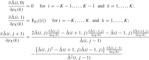
for k = 1, …, K, i = −K + j, …, K − j and j = l, …,K.
When Δ(i, j) = 0 the statistic t(i, j) asymptotically follows a N(0, 1) (provided, in particular, that E![]() exists). If, in contrast, Δ(i, j) ≠ 0 then
exists). If, in contrast, Δ(i, j) ≠ 0 then ![]() a.s. when n → ∞. We can reject the hypothesis Δ(i, j) = 0 at level α if |t(i, j)| is beyond the (1 − α/2)-quantile of a N(0, 1). We can also automatically detect a corner of small values in the table, (Tl) say, giving the t(i, j), if no entry in this corner is greater than this (1 − α/2)-quantile in absolute value. This practice does not correspond to any formal test at level α, but allows a small number of plausible values to be selected for the orders P and Q.
a.s. when n → ∞. We can reject the hypothesis Δ(i, j) = 0 at level α if |t(i, j)| is beyond the (1 − α/2)-quantile of a N(0, 1). We can also automatically detect a corner of small values in the table, (Tl) say, giving the t(i, j), if no entry in this corner is greater than this (1 − α/2)-quantile in absolute value. This practice does not correspond to any formal test at level α, but allows a small number of plausible values to be selected for the orders P and Q.
Illustration of the Corner Method
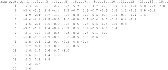
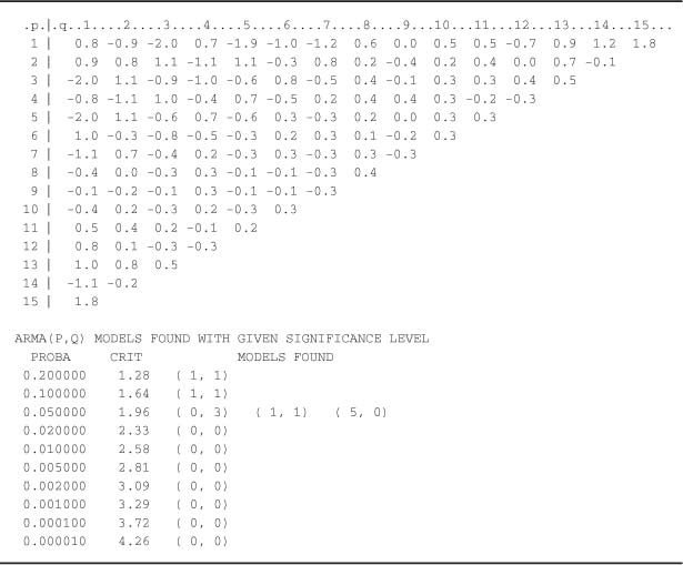
For a simulation of size n = 1000 of the ARMA(2, 1)-GARCH(1, 1) model (5.8) we obtain the following table:
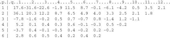
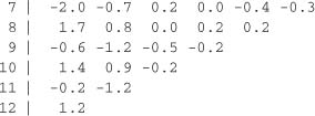
A corner of values which can be viewed as plausible realizations of the N(0, 1) can be observed. This comer corresponds to the rows 3,4,... and the columns 2, 3, …, leading us to select the ARMA (2, 1) model. The automatic detection routine for corners of small values gives:
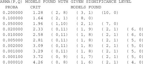
We retrieve the orders (P, Q) = (2, 1) of the simulated model, but also other plausible orders. This is not surprising since the ARMA(2, 1) model can be well approximated by other ARMA models, such as an AR(6), an MA(11) or an ARMA(1, 8) (but in practice, the ARMA(2, 1) should be preferred for parsimony reasons).
5.3 Identifying the GARCH Orders of an ARMA-GARCH Model
The Box-Jenkins methodology described in Chapter 1 for ARMA models can be adapted to GARCH(p, q) models. In this section we consider only the identification problem. First suppose that the observations are drawn from a pure GARCH. The choice of a small number of plausible values for the orders p and q can be achieved in several steps, using various tools:
(i) inspection of the sample autocorrelations and sample partial autocorrelations of ![]() ;
;
(ii) inspection of statistics that are functions of the sample autocovariances of ![]() (corner method, epsilon algorithm, …);
(corner method, epsilon algorithm, …);
(iii) use of information criteria (AIC, BIC, …);
(iv) tests of the significance of certain coefficients;
(v) analysis of the residuals.
Steps (iii) and (v), and to a large extent step (iv), require the estimation of models, and are used to validate or modify them. Estimation of GARCH models will be studied in detail in the forthcoming chapters. Step (i) relies on the ARMA representation for the square of a GARCHprocess.In particular, if (![]() t) Is an ARCH(q) process, then the theoretical partial autocorrelation function r
t) Is an ARCH(q) process, then the theoretical partial autocorrelation function r![]() 2 (·) of
2 (·) of ![]() satisfies
satisfies
For mixed models, the corner method can be used.
5.3.1 Corner Method in the GARCH Case
To Identify the orders of a GARCH(p, q) process, one can use the fact that (![]() ) follows an ARMA
) follows an ARMA ![]() ,
,![]() with
with ![]() = max(p, q) and
= max(p, q) and ![]() = p. In the case of a pure GARCH, (
= p. In the case of a pure GARCH, (![]() t) = (Xt) is observed. The asymptotic variance of the SACRs of
t) = (Xt) is observed. The asymptotic variance of the SACRs of ![]() can be estimated by the method described in Section 5.2.2. The table of studentized statistics for the corner method follows, as described in the previous section. The problem is then to detect at least one comer of normal values starting from the row
can be estimated by the method described in Section 5.2.2. The table of studentized statistics for the corner method follows, as described in the previous section. The problem is then to detect at least one comer of normal values starting from the row ![]() + 1 and the column
+ 1 and the column ![]() + 1 of the table, under the constraints
+ 1 of the table, under the constraints ![]() ≥ 1 (because max(p, q) ≥ q ≥ 1) and
≥ 1 (because max(p, q) ≥ q ≥ 1) and ![]() ≥
≥ ![]() . This leads to selection of GARCH (p, q) models such that (p, q) =
. This leads to selection of GARCH (p, q) models such that (p, q) = ![]() ,
, ![]() when
when ![]() <
< ![]() and (p, q) = (
and (p, q) = (![]() ,1), (p, q) = (
,1), (p, q) = (![]() ,2), …,(p, q) =
,2), …,(p, q) = ![]() ,
, ![]() when
when ![]() ≥
≥![]() .
.
In the ARMA-GARCH case the ![]() t are unobserved but can be approximated by the ARMA residuals. Alternatively, to avoid the ARMA estimation, residuals from fitted ARs, as described in steps 1 and 3 of the algorithm of Section 5.2.1, can be used.
t are unobserved but can be approximated by the ARMA residuals. Alternatively, to avoid the ARMA estimation, residuals from fitted ARs, as described in steps 1 and 3 of the algorithm of Section 5.2.1, can be used.
A Pure GARCH
Consider a simulation of size n = 5000 of the GARCH (2, 1) model
where (ηt) is a sequence of iid N (0, 1) variables, ω = 1, α = 0.1, β1 = 0.05 and β2 = 0.8.
The table of studentized statistics for the corner method is as follows:
A corner of plausible N (0, 1) values Is observed starting from the row ![]() + 1 = 3 and the column
+ 1 = 3 and the column ![]() + 1 = 3, which corresponds to GARCH(p, q) models such that (max(p, q), p) = (2, 2), that
+ 1 = 3, which corresponds to GARCH(p, q) models such that (max(p, q), p) = (2, 2), that
Is, (p, q) = (2, 1) or (p, q) = (2, 2). A small number of other plausible values are detected for (p, q)
An ARMA-GARCH
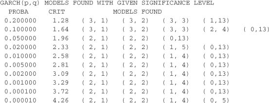
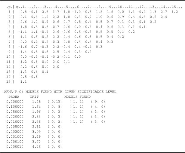
Let us resume the simulation of size n = 1000 of the ARMA(2, 1)-GARCH (1, 1) model (5.8). The table of studentized statistics for the corner method, applied to the SACRs of the observed process, was presented in Section 5.2.3. A small number of ARMA models, Including the ARMA(2, 1), was selected. Let e1 + p0, …, en denote the residuals when an AR(p0) is fitted to the observations, the order p0 being selected using an Information criterion.4 Applying the corner method again, but this time on the SACRs of the squared residuals ![]() , and estimating the covariances between the SACRs by the multivariate AR spectral approximation, as described in Section 5.2.2, we obtain the following table:
, and estimating the covariances between the SACRs by the multivariate AR spectral approximation, as described in Section 5.2.2, we obtain the following table:
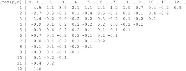
A corner of values compatible with the N (0, 1) is observed starting from row 2 and column 2, which corresponds to a GARCH(1, 1) model. Another comer can be seen below row 2, which corresponds to a GARCH(0, 2) = ARCH(2) model. In practice, in this identification step, at least these two models would be selected. The next step would be the estimation of the selected models, followed by a validation step involving testing the significance of the coefficients, examining the residuals and comparing the models via information criteria. This validation step allows a final model to be retained which can be used for prediction purposes.
5.4 Lagrange Multiplier Test for Conditional Homoscedastlclty
To test linear restrictions on the parameters of a model, the most widely used tests are the Wald test, the Lagrange multiplier (LM) test and likelihood ratio (LR) test. The LM test, also referred to as the Rao test or the score test, is attractive because it only requires estimation of the restricted model (unlike the Wald and LR tests which will be studied in Chapter 8), which is often much easier than estimating the unrestricted model. We start by deriving the general form of the LM test. Then we present an LM test for conditional homoscedasticity in Section 5.4.2.
5.4.1 General Form of the LM Test
Consider a parametric model, with true parameter value θ0 ![]()
![]() d, and a null hypothesis
d, and a null hypothesis
where R is a given s × d matrix of full rank s, and r is a given s × 1 vector. This formulation allows one to test, for instance, whether the first s components of θ0 are null (it suffices to set R = [ls : 0S × (d − s)] and r = 0s). Let ![]() n(θ) denote the log-likelihood of observations X1, …, Xn. We assume the existence of unconstrained and constrained (by H0) maximum likelihood estimators, respectively satisfying
n(θ) denote the log-likelihood of observations X1, …, Xn. We assume the existence of unconstrained and constrained (by H0) maximum likelihood estimators, respectively satisfying
Under some regularity assumptions (which will be discussed in detail in Chapter 7 for the GARCH(p, q) model) the score vector satisfies a central limit theorem and we have
where ![]() is the Fisher information matrix. To derive the constrained estimator we introduce the Lagrangian
is the Fisher information matrix. To derive the constrained estimator we introduce the Lagrangian
We have
The first-order conditions give
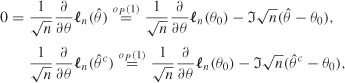
The second convergence in (5.14) thus shows that under H0,
Using the convention ![]() for a = b + c, asymptotic expansions entail, under usual regularity conditions (more rigorous statements will be given in Chapter 7),
for a = b + c, asymptotic expansions entail, under usual regularity conditions (more rigorous statements will be given in Chapter 7),
which, by subtraction, gives
Finally, (5.15) and (5.16) imply
and then
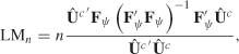
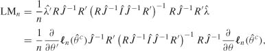
Thus, under H0, the test statistic
asymptotically follows a ![]() , provided that
, provided that ![]() is an estimator converging in probability to
is an estimator converging in probability to ![]() . In general one can take
. In general one can take
The critical region of the LM test at the asymptotic level α is {LMn > ![]() (l − α)}.
(l − α)}.
The Case where the LMn Statistic Takes the Form nR2
Implementation of an LM test can sometimes be extremely simple. Consider a nonlinear conditionally homoscedastic model in which a dependent variable Yt is related to its past values and to a vector of exogenous variables Xt by Yt = Fθ0(Wt) + ![]() t, where
t, where ![]() t is iid
t is iid ![]() and Wt = (Xt, Yt − 1, …). Assume, in addition, that Wt and
and Wt = (Xt, Yt − 1, …). Assume, in addition, that Wt and ![]() t are independent. We wish to test the hypothesis
t are independent. We wish to test the hypothesis
where
To retrieve the framework of the previous section, let R = [0s ×(d × s) : Is] and note that
where Σλ = (![]() 22)−1 and
22)−1 and ![]() 22 = R
22 = R![]() − 1 R′ is the bottom right-hand block of
− 1 R′ is the bottom right-hand block of ![]() − 1. Suppose that
− 1. Suppose that ![]() does not depend on ψ0. With a Gaussian likelihood (Exercise 5.9) we have
does not depend on ψ0. With a Gaussian likelihood (Exercise 5.9) we have
where ![]() t(θ) = Yt − Fθ(Wt),
t(θ) = Yt − Fθ(Wt), ![]() and
and
Partition ![]() into blocks as
into blocks as
where ![]() 11 and
11 and ![]() 22 are square matrices of respective sizes d − s and s. Under the assumption that the information matrix
22 are square matrices of respective sizes d − s and s. Under the assumption that the information matrix ![]() is block-diagonal (that is,
is block-diagonal (that is, ![]() 12 = 0), we have
12 = 0), we have ![]() where
where ![]() 22 = R
22 = R![]() R′, which entails Σλ =
R′, which entails Σλ = ![]() 22. We can then choose
22. We can then choose
as a consistent estimator of Σλ. We end up with
which is nothing other than n times the uncentered determination coefficient in the regression of ![]() on the variables
on the variables ![]() for i = 1, …, s (Exercise 5.10).
for i = 1, …, s (Exercise 5.10).
LM Test with Auxiliary Regressions
We extend the previous framework by allowing ![]() 12 to be not equal to zero. Assume that σ2 does not depend on θ. In view of Exercise 5.9, we can then estimate Σλ by5
12 to be not equal to zero. Assume that σ2 does not depend on θ. In view of Exercise 5.9, we can then estimate Σλ by5
where
Suppose the model is linear under the constraint H0, so that
up to some negligible terms.
Now consider the linear regression
Exercise 5.10 shows that, in this auxiliary regression, the LM statistic for testing the hypothesis
is given by
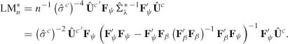
This statistic is precisely the LM test statistic for the hypothesis H0 : ψ = 0 in the initial model. From Exercise 5.10, the LM test statistic of the hypothesis H0* : ψ* = 0 in model (5.19) can also be written as
where ![]() with
with ![]() * = (F′F)−1 F′Y. We finally obtain the so-called Breusch-Godfrey form of the LM statistic by interpreting LMn* in (5.20) as n times the determination coefficient of the auxiliary regression
* = (F′F)−1 F′Y. We finally obtain the so-called Breusch-Godfrey form of the LM statistic by interpreting LMn* in (5.20) as n times the determination coefficient of the auxiliary regression
where ![]() c is the vector of residuals in the regression of Y on the columns of Fβ.
c is the vector of residuals in the regression of Y on the columns of Fβ.
Indeed, in the two regressions (5.19) and (5.21), the vector of residuals is ![]() =
= ![]() , because . Finally, we note that the determination coefficient is centered (in other words, it is R2 as provided by standard statistical software) when a column of Fβ is constant.
, because . Finally, we note that the determination coefficient is centered (in other words, it is R2 as provided by standard statistical software) when a column of Fβ is constant.
Quasi-LM Test
When ![]() n(θ) is no longer supposed to be the log-likelihood, but only the quasi-log-likelihood (a thorough study of the quasi-likelihood for GARCH models will be made in Chapter 7), the equations can in general be replaced by
n(θ) is no longer supposed to be the log-likelihood, but only the quasi-log-likelihood (a thorough study of the quasi-likelihood for GARCH models will be made in Chapter 7), the equations can in general be replaced by
where
It is then recommended that (5.17) be replaced by the more complex, but more robust, expression
where ![]() and
and ![]() are consistent estimators of I and J. A consistent estimator of J is obviously obtained as a sample mean. Estimating the long-run variance I requires more involved methods, such as those described on page 105 (HAC or other methods).
are consistent estimators of I and J. A consistent estimator of J is obviously obtained as a sample mean. Estimating the long-run variance I requires more involved methods, such as those described on page 105 (HAC or other methods).
5.4.2 LM Test for Conditional Homoscedasticity
Consider testing the conditional homoscedasticity assumption
in the ARCH(q) model
At the parameter value θ = (ω, α1, …, αq) the quasi-log-likelihood is written, neglecting unimportant constants, as
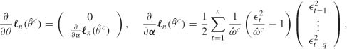
with the convention ![]() t − = 0 for t ≤ 0. The constrained quasi-maximum likelihood estimator is
t − = 0 for t ≤ 0. The constrained quasi-maximum likelihood estimator is
![]() where
where ![]() 6.
6.
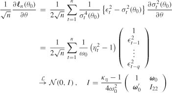
At θ0 = (ω0, …, 0), the score vector satisfies
under H0, where ω0 = (ω0, …, ω0)′ ![]()
![]() q and I22 is a matrix whose diagonal elements are
q and I22 is a matrix whose diagonal elements are ![]() with kn = E
with kn = E![]() , and whose other entries are equal to
, and whose other entries are equal to ![]() . The bottom right-hand block of I− 1 is thus
. The bottom right-hand block of I− 1 is thus
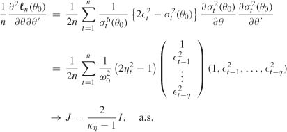
In addition, we have
From (5.23), using estimators of I and J such that we obtain
Using (5.24) and noting that
we obtain
Equivalence with a Portmanteau Test
Using
It follows from (5.25) that
which shows that the LM test is equivalent to a portmanteau test on the squares.
Expression in Terms of R2
To establish a connection with the linear model, write
where Y is the n × l vector ![]() , and X is the n × (q + 1) matrix with first column 1/
, and X is the n × (q + 1) matrix with first column 1/![]() c and (i + l)th column
c and (i + l)th column ![]() . Estimating I by (
. Estimating I by (![]() η − l)n− 1 X′X, where
η − l)n− 1 X′X, where ![]() η − 1 = n− 1 Y′Y, we obtain
η − 1 = n− 1 Y′Y, we obtain
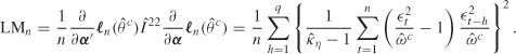
which can be Interpreted as n times the determination coefficient In the linear regression of Y on the columns of X. Because the determination coefficient is invariant by linear transformation of the variables (Exercise 5.11), we simply have LMn = nR2 where R2 is the determination coefficient7 of the regression of ![]() on a constant and q lagged variables
on a constant and q lagged variables ![]() . Under the null hypothesis of conditional homoscedasticity, LMn asymptotically follows a
. Under the null hypothesis of conditional homoscedasticity, LMn asymptotically follows a ![]() . The version of the LM statistic given in (5.27) differs from the one given in (5.25) because (5.24) is not satisfied when I is replaced by (
. The version of the LM statistic given in (5.27) differs from the one given in (5.25) because (5.24) is not satisfied when I is replaced by (![]() η − 1)n− 1 X′X.
η − 1)n− 1 X′X.
5.5 Application to Real Series
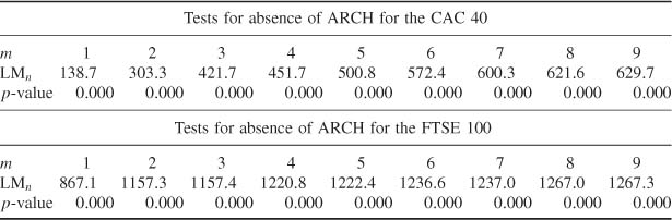
Consider the returns of the CAC 40 stock index from March 2, 1990 to December 29, 2006 (4245 observations) and of the FTSE 100 index of the London Stock Exchange from April 3, 1984 to April 3, 2007 (5812 observations). The correlograms for the returns and squared returns are displayed in Figure 5.7. The bottom correlograms of Figure 5.7, as well as the portmanteau tests of Table 5.4, clearly show that, for the two indices, the strong white noise assumption cannot be sustained. These portmanteau tests can be considered as versions of LM tests for conditional homoscedasticity (see Section 5.4.2). Table 5.5 displays the nR2 version of the LM test of Section 5.4.2. Note that the two versions of the LM statistic are quite different but lead to the same unambiguous conclusions: the hypothesis of no ARCH effect must be rejected, as well as the hypothesis of absence of autocorrelation for the CAC 40 or FTSE 100 returns.
The first correlogram of Figure 5.7 and the first part of Table 5.6 lead us to think that the CAC 40 series is fairly compatible with a weak white noise structure (and hence with a GARCH structure). Recall that the 95% significance bands, shown as dotted lines on the upper correlograms of Figure 5.7, are valid under the strong white noise assumption but may be misleading for weak white noises (such as GARCH). The second part of Table 5.6 displays classical Ljung-Box tests for noncorrelation. It may be noted that the CAC 40 returns series does not pass the classical portmanteau tests.8 This does not mean, however, that the white noise assumption should be
Figure 5.7 Correlograms of returns and squared returns of the CAC 40 index (March 2, 1990 to December 29, 2006) and the FTSE 100 index (April 3, 1984 to April 3, 2007).
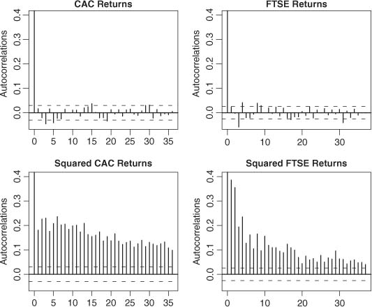
Table 5.4 Portmanteau tests on the squared CAC 40 returns (March 2, 1990 to December 29, 2006) and FTSE 100 returns (April 3, 1984 to April 3, 2007).
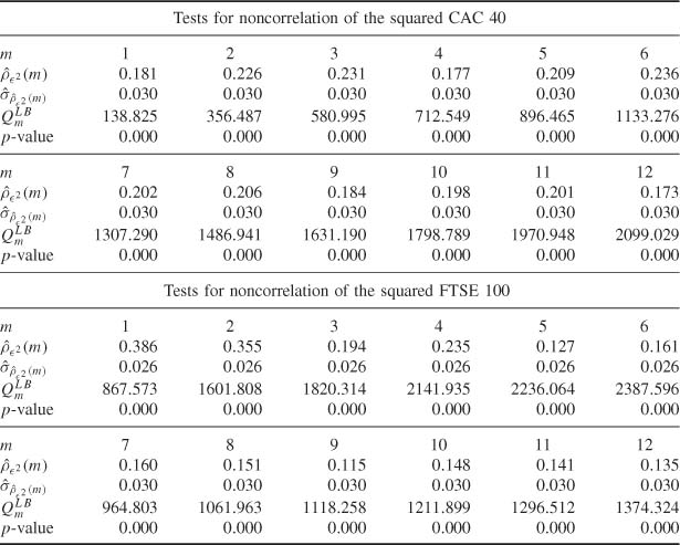
Table 5.5 LM tests for conditional homoscedasticity of the CAC 40 and FTSE 100.
rejected. Indeed, we know that such classical portmanteau tests are invalid for conditionally heteroscedastic series.
Table 5.7 is the analog of Table 5.6 for the FTSE 100 index. Conclusions are more disputable in this case. Although some p-values of the upper part of Table 5.7 are slightly less than 5%, one cannot exclude the possibility that the FTSE 100 index is a weak (GARCH) white noise.
Table 5.6 Portmanteau tests on the CAC 40 (March 2, 1990 to December 29, 2006).
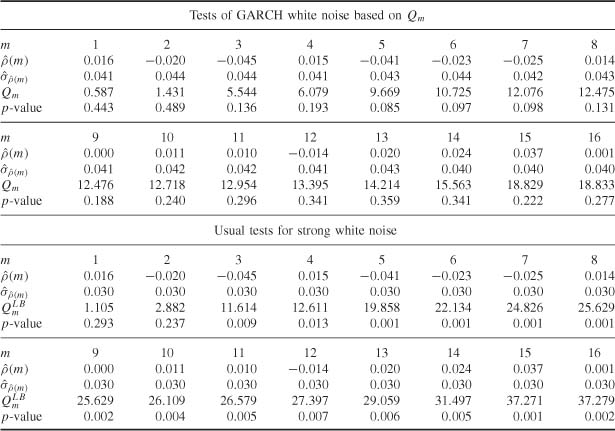
Table 5.7 Portmanteau tests on the FTSE 100 (April 3, 1984 to April 3, 2007).
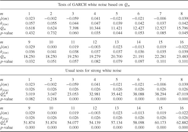
Table 5.8 Studentized statistics for the comer method for the CAC 40 series and selected ARMA orders.
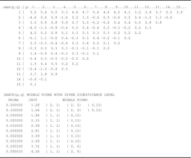
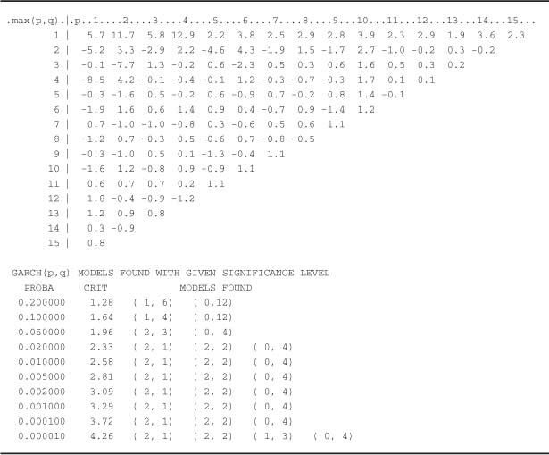
On the other hand, the assumption of strong white noise can be categorically rejected, the p-values (bottom of Table 5.7) being almost equal to zero. Table 5.8 confirms the identification of an ARMA(0, 0) process for the CAC 40. Table 5.9 would lead us to select an ARMA(0, 0), ARMA(1, 1), AR(3) or MA(3) model for the FTSE 100. Recall that this a priori identification step should be completed by an estimation of the selected models, followed by a validation step. For the CAC 40, Table 5.10 indicates that the most reasonable GARCH model is simply the GARCH(1, 1). For the FTSE 100, plausible models are the GARCH(2, 1), GARCH(2, 2), GARCH(2, 3), or ARCH(4), as can be seen from Table 5.11. The choice between these models is the object of the estimation and validation steps.
In this chapter, we have adapted tools generally employed to deal with the identification of ARMA models. Correlograms and partial correlograms are studied in depth in the book by Brockwell and Davis (1991). In particular, they provide a detailed proof for the Bartlett formula giving the asymptotic behavior of the sample autocorrelations of a strong linear process.
Table 5.9 Studentized statistics for the comer method for the FTSE 100 series and selected ARMA orders.
The generalized Bartlett formula (B.15) was established by Francq and Zakoïan (2009d). The textbook by Li (2004) can serve as a reference for the various portmanteau adequacy tests, as well as Godfrey (1988) for the LM tests. It is now well known that tools generally used for the identification of ARMA models should not be directly used in presence of conditional net-eroscedasticity, or other forms of dependence in the linear innovation process (see, for instance, Diebold, 1986; Romano and Thombs, 1996; Berlinet and Francq, 1997; or Francq, Roy and Zakoïan, 2005). The corner method was proposed by Béguin, Gourieroux and Monfort (1980) for the identification of mixed ARMA models. There are many alternatives to the corner method, in particular the epsilon algorithm (see Berlinet, 1984) and the generalized autocorrelations of Glasbey (1982).
Additional references on tests of ARCH effects are Engle (1982, 1984), Bera and Higgins (1997) and Li (2004).
In this chapter we have assumed the existence of a fourth-order moment for the observed process. When only the second-order moment exists, Basrak, Davis and Mikosch (2002) showed in particular that the sample autocorrelations converge very slowly. When even the second-order moment does not exist, the sample autocorrelations have a degenerate asymptotic distribution.
Table 5.10 Studentized statistics for the corner method for the squared CAC 40 series and selected GARCH orders.
Concerning the HAC estimators of a long-run variance matrix, see, for instance, Andrews (1991) and Andrews and Monahan (1992). The method based on the spectral density at 0 of an AR model follows from Berk (1974). A comparison with the HAC method is proposed in den Hann and Levin (1997).
5.1 (Asymptotic behavior of the SACVs of a martingale difference)
Let (![]() t) denote a martingale difference sequence such that E
t) denote a martingale difference sequence such that E![]() < ∞ and
< ∞ and ![]() . By applying Corollary A.l, derive the asymptotic distribution of nl / 2
. By applying Corollary A.l, derive the asymptotic distribution of nl / 2 ![]() (h) for h ≠ 0.
(h) for h ≠ 0.
5.2 (Asymptotic behavior of n1/2 ![]() (1) for an ARCHQ) process)
(1) for an ARCHQ) process)
Consider the stationary nonanticipative solution of an ARCH(1) process
Table 5.11 Studentized statistics for the corner method for the squared FTSE 100 series and selected GARCH orders.
where (ηt) is a strong white noise with unit variance and μ4α2 < 1 with. Derive the asymptotic distribution of n1/2![]() (l).
(l).
5.3 (Asymptotic behavior of n1/2![]() (1) for an ARCH(1) process)
(1) for an ARCH(1) process)
For the ARCH(l) model of Exercise 5.2, derive the asymptotic distribution of n1/2![]() (l). What is the asymptotic variance of this statistic when α = 0? Draw this asymptotic variance as a function of α and conclude accordingly.
(l). What is the asymptotic variance of this statistic when α = 0? Draw this asymptotic variance as a function of α and conclude accordingly.
5.4 (Asymptotic behavior of the SACRs of a GARCH (1, 1) process)
For the GARCH(1, 1) model of Exercise 2.8, derive the asymptotic distribution of n1/2![]() (h), for h ≠ 0 fixed.
(h), for h ≠ 0 fixed.
5.5 (Moment of order 4 of a GARCH(1, 1) process)
For the GARCH(1, 1) model of Exercise 2.8, compute E![]() t
t![]() t + 1
t + 1![]() s
s![]() s + 2.
s + 2.
5.6 (Asymptotic covariance between the SACRs of a GARCH (1, 1) process)
For the GARCH(1, 1) model of Exercise 2.8, compute
5.7 (First five SACRs of a GARCH(l, 1) process)
Evaluate numerically the asymptotic variance of the vector ![]()
![]() 5 of the first five SACRs of the GARCH(1, 1) model defined by
5 of the first five SACRs of the GARCH(1, 1) model defined by
5.8 (Generalized Bartlett formula for an MA(q)-ARCH(X) process)
Suppose that Xt follows an MA(q) of the form
where the error term is an ARCH(l) process
How is the generalized Bartlett formula (B.15) expressed for i = j > q?
5.9 (Fisher information matrix for dynamic regression model)
In the regression model Yt = Fθ0(Wt) + ![]() t introduced on page 112, suppose that (
t introduced on page 112, suppose that (![]() t) is a
t) is a ![]() (0,
(0,![]() ) white noise. Suppose also that the regularity conditions entailing (5.14) hold. Give an explicit form to the blocks of the matrix I, and consider the case where σ2 does not depend on θ.
) white noise. Suppose also that the regularity conditions entailing (5.14) hold. Give an explicit form to the blocks of the matrix I, and consider the case where σ2 does not depend on θ.
5.10 (LM tests in a linear regression model)
Consider the regression model
where Y = (Y1, …, Yn) is the dependent vector variable, Xi is an n × ki matrix of explicative variables with rank ki (i = 1, 2), and the vector U is a N(0, σ2In) error term. Derive the LM test of the hypothesis H0 : β2 = 0. Consider the case X′1X2 = 0 and the general case.
5.11 (Centered and uncentered R2)
Consider the regression model
where the ![]() t are iid, centered, and have a variance σ2 > 0. Let Y = (Y1, …, Yn)′ be the vector of dependent variables, X = (Xif) the n × k matrix of explanatory variables,
t are iid, centered, and have a variance σ2 > 0. Let Y = (Y1, …, Yn)′ be the vector of dependent variables, X = (Xif) the n × k matrix of explanatory variables, ![]() = (
= (![]() 1, …,
1, …, ![]() n)′ the vector of the error terms and β = (β1, …, βk)′ the parameter vector. Let Px = X(X′X)−1 X′ denote the orthogonal projection matrix on the vector subspace generated by the columns of X.
n)′ the vector of the error terms and β = (β1, …, βk)′ the parameter vector. Let Px = X(X′X)−1 X′ denote the orthogonal projection matrix on the vector subspace generated by the columns of X.
The uncentered determination coefficient is defined by
and the (centered) determination coefficient is defined by
Let T denote a k × k invertible matrix, c a number different from 0 and d any number.
Let ![]() = cY + de and
= cY + de and ![]() = XT. Show that if
= XT. Show that if ![]() = 0 and if e belongs to the vector subspace generated by the columns of X, then
= 0 and if e belongs to the vector subspace generated by the columns of X, then ![]() defined by (5.29) is equal to the determination coefficient in the regression of
defined by (5.29) is equal to the determination coefficient in the regression of ![]() on the columns of
on the columns of ![]() .
.
5.12 (Identification of the DAX and the S&P 500)
From the address http://fr.biz.yahoo.com//bourse/accueil.html download the series of DAX and S&P 500 stock indices. Carry out a study similar to that of Section 5.5 and deduce a selection of plausible models.
1 For any sequence (Zn) of random vectors of size d, ![]() if and only if, for all λ
if and only if, for all λ ![]()
![]() d, we have
d, we have ![]()
2 The asymptotic distribution of ![]() is
is ![]() . The Box and Pierce (1970) statistic
. The Box and Pierce (1970) statistic ![]() has the same asymptotic distribution, but the
has the same asymptotic distribution, but the ![]() statistic is believed to perform better for finite samples.
statistic is believed to perform better for finite samples.
3Comparing ![]() and
and ![]() for j ≠j′ (that is, entries of different rows in table
for j ≠j′ (that is, entries of different rows in table ![]() ) is all the more difficult as these are determinants of matrices of different sizes.
) is all the more difficult as these are determinants of matrices of different sizes.
4 One can also use the innovations algorithm of Brockwell and Davis (1991, p. 172) for rapid fitting of MA models. Alternatively, one of the previously selected ARMA models, for instance the ARMA(2, 1), can be used to approximate the innovations.
5 For a partitioned invertible matrix ![]() , where A11 and A22 are invertible square blocks, the bottom right-hand block of A−1 is written as
, where A11 and A22 are invertible square blocks, the bottom right-hand block of A−1 is written as ![]() (Exercise 6.7).
(Exercise 6.7).
6 Indeed, the function σ2 Φ x / σ2 + n log σ2 reaches its minimum at σ2 = x / n.
7We mean here the centered determination coefficient (the one usually given by standard software) not the uncentered one as was the case in Section 5.4.1. There is sometimes confusion between these coefficients in the literature.
8 Classical portmanteau tests are those provided by standard commercial software, in particular those of the table entitled ‘Autocorrelation Check for White Noise’ of the arima procedure in sas.