Classical Time Series Models and Financial Series
The standard time series analysis rests on important concepts such as stationarity, autocorrelation, white noise, innovation, and on a central family of models, the autoregressive moving average (ARMA) models. We start by recalling their main properties and how they can be used. As we shall see, these concepts are insufficient for the analysis of financial time series. In particular, we shall introduce the concept of volatility, which is of crucial importance in finance.
In this chapter, we also present the main stylized facts (unpredictability of returns, volatility clustering and hence predictability of squared returns, leptokurticity of the marginal distributions, asymmetries, etc.) concerning financial series.
Stationarity plays a central part in time series analysis, because it replaces in a natural way the hypothesis of independent and identically distributed (iid) observations in standard statistics.
Consider a sequence of real random, variables (Xt)t![]()
![]() , defined on the same probability space. Such a sequence is called a time series, and is an example of a discrete-time stochastic process.
, defined on the same probability space. Such a sequence is called a time series, and is an example of a discrete-time stochastic process.
We begin by introducing two standard notions of stationarity.
Definition 1.1 (Strict stationarity) The process (Xt) is said to be strictly stationary if the vectors (X1, …, Xk)′ and (X1+h, …, Xk+h)′ have the same joint distribution, for any k ![]()
![]() and any h
and any h ![]()
![]() .
.
The following notion may seem less demanding, because it only constrains the first two moments of the variables Xt, but contrary to strict stationarity, it requires the existence of such moments.
Definition 1.2 (Second-order stationarity) The process (Xt) is said to be second-order stationary if:
(i) E ![]() < ∞ ,
< ∞ ,![]() t
t![]()
![]()
(ii) EXt = m, ![]() t
t![]()
![]()
(iii) Cov(Xt, Xt+h) = γX(h), ![]() t, h
t, h ![]()
![]()
The function γx(·) (ρx(·) : = γx(·)/γx(0)) is called the autocovariance function (autocorrelation function) of (Xt).
The simplest example of a second-order stationary process is white noise. This process is particularly important because it allows more complex stationary processes to be constructed.
Definition 1.3 (Weak white noise) The process (![]() t) is called weak white noise if for some positive constant σ2:
t) is called weak white noise if for some positive constant σ2:
(i) E![]() t = 0, ∀
t = 0, ∀ ![]() t
t ![]()
![]()
(ii)E ![]() = σ2,
= σ2, ![]() t
t ![]()
![]()
(iii) Cov(![]() t,
t, ![]() t+h) = 0,
t+h) = 0, ![]() t, h
t, h ![]()
![]() , h ≠ 0.
, h ≠ 0.
Remark 1.1 (Strong white noise) It should be noted that no independence assumption is made in the definition of weak white noise. The variables at different dates are only uncorrelated and the distinction is particularly crucial for financial time series. It is sometimes necessary to replace hypothesis (iii) by the stronger hypothesis
(iii′) the variables ![]() t and
t and ![]() t+h are independent and identically distributed.
t+h are independent and identically distributed.
The process (![]() t) is then said to be strong white noise.
t) is then said to be strong white noise.
Estimating Autocovariances
The classical time series analysis is centered on the second-order structure of the processes. Gaussian stationary processes are completely characterized by their mean and their autocovariance function. For non-Gaussian processes, the mean and autocovariance give a first idea of the temporal dependence structure. In practice, these moments are unknown and are estimated from a realization of size n of the series, denoted X1, …, Xn. This step is preliminary to any construction of an appropriate model. To estimate γ(h), we generally use the sample autocovariance defined, for 0 ≤ h ≤ n, by
where ![]() denotes the sample mean. We similarly define the sample autocorrelation function by
denotes the sample mean. We similarly define the sample autocorrelation function by ![]() (h) =
(h) = ![]() (h) /
(h) /![]() (0) for |h| < n.
(0) for |h| < n.
The previous estimators have finite-sample bias but are asymptotically unbiased. There are other similar estimators of the autocovariance function with the same asymptotic properties (for instance, obtained by replacing 1/n by l/(n − h)). However, the proposed estimator is to be preferred over others because the matrix (![]() (i − j)) is positive semi-definite (see Brockwell and Davis, 1991, p. 221).
(i − j)) is positive semi-definite (see Brockwell and Davis, 1991, p. 221).
It is of course not recommended to use the sample autocovariances when h is close to n, because too few pairs (Xj, Xj + h) are available. Box, Jenkins and Reinsel (1994, p. 32) suggest that useful estimates of the autocorrelations can only be made if, approximately, n > 50 and h < n/4.
It is often of interest to know - for instance, in order to select an appropriate model - if some or all the sample autocovariances are significantly different from 0. It is then necessary to estimate the covariance structure of those sample autocovariances. We have the following result (see Brockwell and Davis, 1991, pp. 222, 226).
Theorem 1.1 (Bartlett’s formulas for a strong linear process) Let (Xt) be a linear process satisfying
where (![]() t) is a sequence of iid variables such that
t) is a sequence of iid variables such that
Appropriately normalized, the sample autocovariances and autocorrelations are asymptotically normal, with asymptotic variances given by the Bartlett formulas:
and
Formula (1.2) still holds under the assumptions
In particular, if Xt = ![]() t and E
t and E ![]() , < ∞ we have
, < ∞ we have
The assumptions of this theorem are demanding, because they require a strong white noise (![]() t). An extension allowing the strong linearity assumption to be relaxed is proposed in Appendix B.2. For many nonlinear processes, in particular the ARCH processes studies in this book, the asymptotic covariance of the sample autocovariances can be very different from. (1.1) (Exercises 1.6 and 1.8). Using the standard Bartlett formula can lead to specification errors (see Chapter 5).
t). An extension allowing the strong linearity assumption to be relaxed is proposed in Appendix B.2. For many nonlinear processes, in particular the ARCH processes studies in this book, the asymptotic covariance of the sample autocovariances can be very different from. (1.1) (Exercises 1.6 and 1.8). Using the standard Bartlett formula can lead to specification errors (see Chapter 5).
The aim of time series analysis is to construct a model for the underlying stochastic process. This model is then used for analyzing the causal structure of the process or to obtain optimal predictions.
The class of ARMA models Is the most widely used for the prediction of second-order stationary processes. These models can be viewed as a natural consequence of a fundamental result due to Wold (1938), which can be stated as follows: any centered, second-order stationary, and ‘purely nondeterministic’ process1 admits an infinite moving-average representation of the form
where (![]() t) is the linear innovation process of (Xt), that is
t) is the linear innovation process of (Xt), that is
where ![]() x(t − 1) denotes the Hilbert space generated by the random variables Xt − 1, Xt − 2, ….2 and E(Xt |
x(t − 1) denotes the Hilbert space generated by the random variables Xt − 1, Xt − 2, ….2 and E(Xt | ![]() x(t − 1)) denotes the orthogonal projection of Xt onto
x(t − 1)) denotes the orthogonal projection of Xt onto ![]() x(t − 1). The sequence of coefficients (ci) is such that
x(t − 1). The sequence of coefficients (ci) is such that ![]() . Note that (
. Note that (![]() t) is a weak white noise.
t) is a weak white noise.
Truncating the infinite sum in (1.3), we obtain the process
called a moving average process of order q, or MA(q). We have
It follows that the set of all finite-order moving averages is dense In the set of second-order stationary and purely nondeterministic processes. The class of ARMA models is often preferred to the MA models for parsimony reasons, because they generally require fewer parameters.
Definition 1.4 (ARMA(p, q) process) A second-order stationary process (Xt) is called ARMA(p, q), where p and q are integers, if there exist real coefficients c, a1, …, ap, b1, …, bq such that,
where (![]() t) is the linear innovation process of (Xt).
t) is the linear innovation process of (Xt).
This definition entails constraints on the zeros of the autoregressive and moving average polynomials, ![]() and
and ![]() (Exercise 1.9). The main attraction of this model, and the representations obtained by successively inverting the polynomials a(·) and b(·), is that it provides a framework for deriving the optimal linear predictions of the process, in much simpler way than by only assuming the second-order stationarity.
(Exercise 1.9). The main attraction of this model, and the representations obtained by successively inverting the polynomials a(·) and b(·), is that it provides a framework for deriving the optimal linear predictions of the process, in much simpler way than by only assuming the second-order stationarity.
Many economic series display trends, making the stationarity assumption unrealistic. Such trends often vanish when the series is differentiated, once or several times. Let ΔXt = Xt − Xt−1 denote the first-difference series, and let ![]() ) denote the differences of order d.
) denote the differences of order d.
Definition 1.5 (ARIMA(p, d, q) process) Let d be a positive integer. The process (Xt) is said to be an ARIMA(p, d, q) process if, for k = 0, …, d − 1, the processes (ΔkXt) are not second-order stationary, and (ΔdXt) is an ARMA(p, q) process.
The simplest ARIMA process is the ARIMA(0, 1, 0), also called the random walk, satisfying
where ![]() t is a weak white noise.
t is a weak white noise.
For statistical convenience, ARMA (and ARIMA) models are generally used under stronger assumptions on the noise than that of weak white noise. Strong ARMA refers to the ARMA model of Definition 1.4 when ![]() t is assumed to be a strong white noise. This additional assumption allows us to use convenient statistical tools developed in this framework, but considerably reduces the generality of the ARMA class. Indeed, assuming a strong ARMA is tantamount to assuming that (i) the optimal predictions of the process are linear ((
t is assumed to be a strong white noise. This additional assumption allows us to use convenient statistical tools developed in this framework, but considerably reduces the generality of the ARMA class. Indeed, assuming a strong ARMA is tantamount to assuming that (i) the optimal predictions of the process are linear ((![]() t) being the strong innovation of (Xt)) and (ii) the amplitudes of the prediction intervals depend on the horizon but not on the observations. We shall see in the next section how restrictive this assumption can be, in particular for financial time series modeling.
t) being the strong innovation of (Xt)) and (ii) the amplitudes of the prediction intervals depend on the horizon but not on the observations. We shall see in the next section how restrictive this assumption can be, in particular for financial time series modeling.
The orders (p, q) of an ARMA process are fully characterized through its autocorrelation function (see Brockwell and Davis, 1991, pp. 89–90, for a proof).
Theorem 1.2 (Characterization of an ARMA process) Let (Xt) denote a second-order stationary process. We have
if and only if (Xt) is an ARMA(p, q) process.
To close this section, we summarize the method for time series analysis proposed in the famous book by Box and Jenkins (1970). To simplify presentation, we do not consider seasonal series, for which SARIMA models can be considered.
Box-Jenkins Methodology
The aim of this methodology is to find the most appropriate ARIMA(p, d, q) model and to use it for forecasting. It uses an iterative six-stage scheme:
(i) a priori identification of the differentiation order d (or choice of another transformation);
(ii) a priori identification of the orders p and q;
(iii) estimation of the parameters (a1, …, ap, b1, …, bq and σ2 = Var ![]() t);
t);
(iv) validation;
(v) choice of a model;
(vi) prediction.
Although many unit root tests have been introduced in the last 30 years, step (i) is still essentially based on examining the graph of the series. If the data exhibit apparent deviations from stationarity, it will not be appropriate to choose d = 0. For instance, if the amplitude of the variations tends
Figure 1.1 CAC 40 Index for the period from March 1, 1990 to October 15, 2008 (4702 observations).
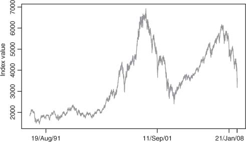
to increase, the assumption of constant variance can be questioned. This may be an indication that the underlying process Is heteroscedastlc.3 If a regular linear trend Is observed, positive or negative, it can be assumed that the underlying process is such that EXt = at + b with a ≠ 0. If this assumption is correct, the first-difference series ΔXt = Xt − Xt−1 should not show any trend (EΔXt = a) and could be stationary. If no other sign of nonstationarity can be detected (such as heteroscedasticity), the choice d = 1 seems suitable. The random walk (whose sample paths may resemble the graph of Figure 1.1), is another example where d = 1 is required, although this process does not have any deterministic trend.
Step (ii) is more problematic. The primary tool is the sample autocorrelation function. If, for Instance, we observe that ![]() (1) is far away from 0 but that for any h > 1,
(1) is far away from 0 but that for any h > 1, ![]() (h) is close to 0,4 then, from Theorem 1.1, it is plausible that ρ(1) ≠ 0 and ρ(h) = 0 for all h > 1. In this case, Theorem. 1.2 entails that Xt is an MA(1) process. To Identify AR processes, the partial autocorrelation function (see Appendix B.l) plays an analogous role. For mixed models (that is, ARMA(p, q) with pq ≠ 0), more sophisticated statistics can be used, as will be seen in Chapter 5. Step (ii) often results in the selection of several candidates (p1, q1), …, (pk, qk for the ARMA orders. These k models are estimated in step (iii), using, for instance, the least-squares method. The aim of step (iv) is to gauge if the estimated models are reasonably compatible with the data. An important part of the procedure is to examine the residuals which, if the model is satisfactory, should have the appearance of white noise. The correlograms are examined and portmanteau tests are used to decide if the residuals are sufficiently close to white noise. These tools will be described in detail in Chapter 5. When the tests on the residuals fail to reject the model, the significance of the estimated coefficients Is studied. Testing the nullity of coefficients sometimes allows the model to be simplified. This step may lead to rejection of all the estimated models, or to consideration of other models, in which case we are brought back to step (i) or (ii). If several models pass the validation step (iv), selection criteria can be used, the most popular being the Akaike (AIC) and Bayeslan (BIC) Information criteria. Complementing these criteria, the predictive properties of the models can be considered: different models can lead to almost equivalent predictive formulas. The parsimony principle would thus lead us to choose the simplest model, the one with the fewest parameters. Other considerations can also come into play: for Instance, models frequently involve a lagged variable at the order 12 for monthly data, but this would seem less natural for weekly data.
(h) is close to 0,4 then, from Theorem 1.1, it is plausible that ρ(1) ≠ 0 and ρ(h) = 0 for all h > 1. In this case, Theorem. 1.2 entails that Xt is an MA(1) process. To Identify AR processes, the partial autocorrelation function (see Appendix B.l) plays an analogous role. For mixed models (that is, ARMA(p, q) with pq ≠ 0), more sophisticated statistics can be used, as will be seen in Chapter 5. Step (ii) often results in the selection of several candidates (p1, q1), …, (pk, qk for the ARMA orders. These k models are estimated in step (iii), using, for instance, the least-squares method. The aim of step (iv) is to gauge if the estimated models are reasonably compatible with the data. An important part of the procedure is to examine the residuals which, if the model is satisfactory, should have the appearance of white noise. The correlograms are examined and portmanteau tests are used to decide if the residuals are sufficiently close to white noise. These tools will be described in detail in Chapter 5. When the tests on the residuals fail to reject the model, the significance of the estimated coefficients Is studied. Testing the nullity of coefficients sometimes allows the model to be simplified. This step may lead to rejection of all the estimated models, or to consideration of other models, in which case we are brought back to step (i) or (ii). If several models pass the validation step (iv), selection criteria can be used, the most popular being the Akaike (AIC) and Bayeslan (BIC) Information criteria. Complementing these criteria, the predictive properties of the models can be considered: different models can lead to almost equivalent predictive formulas. The parsimony principle would thus lead us to choose the simplest model, the one with the fewest parameters. Other considerations can also come into play: for Instance, models frequently involve a lagged variable at the order 12 for monthly data, but this would seem less natural for weekly data.
If the model is appropriate, step (vi) allows us to easily compute the best linear predictions ![]() t(h) at horizon h = 1, 2, … Recall that these linear predictions do not necessarily lead to minimal quadratic errors. Nonlinear models, or nonparametric methods, sometimes produce more accurate predictions. Finally, the Interval predictions obtained in step (vi) of the Box-Jenkins methodology are based on Gaussian assumptions. Their magnitude does not depend on the data, which for financial series is not appropriate, as we shall see.
t(h) at horizon h = 1, 2, … Recall that these linear predictions do not necessarily lead to minimal quadratic errors. Nonlinear models, or nonparametric methods, sometimes produce more accurate predictions. Finally, the Interval predictions obtained in step (vi) of the Box-Jenkins methodology are based on Gaussian assumptions. Their magnitude does not depend on the data, which for financial series is not appropriate, as we shall see.
Modeling financial time series is a complex problem. This complexity is not only due to the variety of the series in use (stocks, exchange rates, interest rates, etc.), to the importance of the frequency of d’observation (second, minute, hour, day, etc) or to the availability of very large data sets. It Is mainly due to the existence of statistical regularities (stylized facts) which are common to a large number of financial series and are difficult to reproduce artificially using stochastic models.
Most of these stylized facts were put forward In a paper by Mandelbrot (1963). Since then, they have been documented, and completed, by many empirical studies. They can be observed more or less clearly depending on the nature of the series and its frequency. The properties that we now present are mainly concerned with daily stock prices.
Let pt denote the price of an asset at time t and let ![]() t = log(pt/pt−1) be the continuously compounded or log return (also simply called the return). The series (
t = log(pt/pt−1) be the continuously compounded or log return (also simply called the return). The series (![]() t) is often close to the series of relative price variations rt = (pt − pt−1)/pt−1, since
t) is often close to the series of relative price variations rt = (pt − pt−1)/pt−1, since ![]() t = log(l + rt). In contrast to the prices, the returns or relative prices do not depend on monetary units which facilitates comparisons between assets. The following properties have been amply commented upon In the financial literature.
t = log(l + rt). In contrast to the prices, the returns or relative prices do not depend on monetary units which facilitates comparisons between assets. The following properties have been amply commented upon In the financial literature.
(1) Nonstationarity of price series. Samples paths of prices are generally close to a random walk without intercept (see the CAC index series5 displayed in Figure 1.1). On the other hand, sample paths of returns are generally compatible with the second-order stationarity assumption. For Instance, Figures 1.2 and 1.3 show that the returns of the CAC Index
Figure 1.2 CAC 40 returns (March 2, 1990 to October 15, 2008). August 19, 1991, Soviet Putsch attempt; September 11, 2001, fall of the Twin Towers; January 21, 2008, effect of the subprime mortgage crisis; October 6, 2008, effect of the financial crisis.
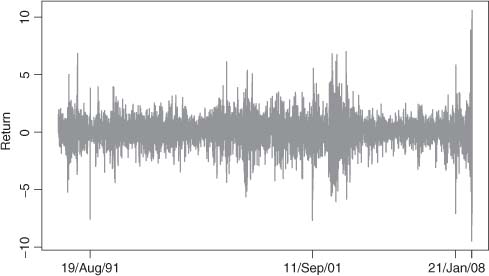
Figure 1.3 Returns of the CAC 40 (January 2, 2008 to October 15, 2008).
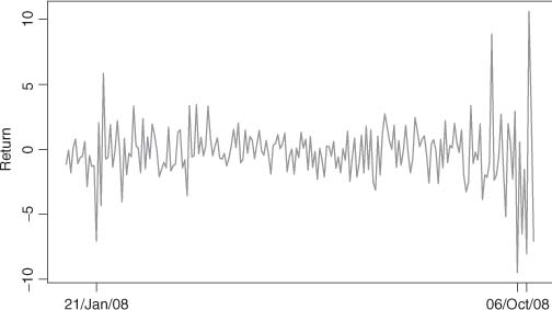
oscillate around zero. The oscillations vary a great deal in magnitude, but are almost constant in average over long subperiods. The recent extreme volatility of prices, induced by the financial crisis of 2008, is worth noting.
(ii) Absence of autocorrelation for the price variations. The series of price variations generally displays small autocorrelations, making it close to a white noise. This is illustrated for the
Figure 1.4 Sample autocorrelations of (a) returns and (b) squared returns of the CAC 40 (January 2, 2008 to October 15, 2008).
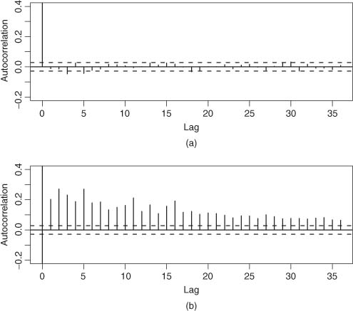
CAC in Figure 1.4(a). The classical significance bands are used here, as an approximation, but we shall see in Chapter 5 that they must be corrected when the noise is not independent. Note that for intraday series, with very small time intervals between observations (measured in minutes or seconds) significant autocorrelations can be observed due to the so-called micro structure effects.
(iii) Autocorrelations of the squared price returns. Squared returns (![]() ) or absolute returns (|
) or absolute returns (|![]() t|) are generally strongly autocorrelated (see Figure 1.4(b)). This property is not incompatible with the white noise assumption for the returns, but shows that the white noise is not strong.
t|) are generally strongly autocorrelated (see Figure 1.4(b)). This property is not incompatible with the white noise assumption for the returns, but shows that the white noise is not strong.
(iv) Volatility clustering. Large absolute returns |![]() t| tend to appear in clusters. This property is generally visible on the sample paths (as in Figure 1.3). Turbulent (high-volatility) subperiods are followed by quiet (low-volatility) periods. These subperiods are recurrent but do not appear in a periodic way (which might contradict the stationarity assumption). In other words, volatility clustering is not incompatible with a homoscedastic (i.e. with a constant variance) marginal distribution for the returns.
t| tend to appear in clusters. This property is generally visible on the sample paths (as in Figure 1.3). Turbulent (high-volatility) subperiods are followed by quiet (low-volatility) periods. These subperiods are recurrent but do not appear in a periodic way (which might contradict the stationarity assumption). In other words, volatility clustering is not incompatible with a homoscedastic (i.e. with a constant variance) marginal distribution for the returns.
(v) Fat-tailed distributions. When the empirical distribution of daily returns is drawn, one can generally observe that it does not resemble a Gaussian distribution. Classical tests typically lead to rejection of the normality assumption at any reasonable level. More precisely, the densities have fat tails (decreasing to zero more slowly than exp(−x2/2)) and are sharply peaked at zero: they are called leptokurtic. A measure of the leptokurticity is the kurtosis coefficient, defined as the ratio of the sample fourth-order moment to the squared sample variance. Asymptotically equal to 3 for Gaussian iid observations, this coefficient is much greater than 3 for returns series. When the time interval over which the returns are computed increases, leptokurticity tends to vanish and the empirical distributions get closer to a Gaussian. Monthly returns, for instance, defined as the sum of daily returns over the month, have a distribution that is much closer to the normal than daily returns. Figure 1.5 compares
Figure 1.5 Kernel estimator of the CAC 40 returns density (solid line) and density of a Gaussian with mean and variance equal to the sample mean and variance of the returns (dotted line).
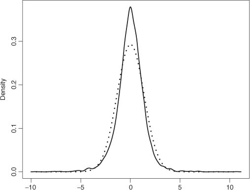
Table 1.1. Sample autocorrelations of returns ![]() t (CAC 40 index, January 2, 2008 to October 15, 2008), of absolute returns |
t (CAC 40 index, January 2, 2008 to October 15, 2008), of absolute returns |![]() t|, sample correlations between
t|, sample correlations between ![]() and |
and |![]() t|, and between
t|, and between ![]() and |
and |![]() t|
t|
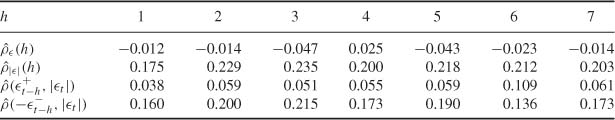
We use here the notation ![]() = max(
= max(![]() t, 0) and
t, 0) and ![]() = min(
= min(![]() t, 0).
t, 0).
a kernel estimator of the density of the CAC returns with a Gaussian density. The peak around zero appears clearly, but the thickness of the tails is more difficult to visualize.
(vi) Leverage effects. The so-called leverage effect was noted by Black (1976), and involves an asymmetry of the impact of past positive and negative values on the current volatility. Negative returns (corresponding to price decreases) tend to increase volatility by a larger amount than positive returns (price increases) of the same magnitude. Empirically, a positive correlation is often detected between ![]() = max(
= max(![]() ,0) and |
,0) and |![]() t+h| (a price increase should entail future volatility increases), but, as shown in Table 1.1, this correlation is generally less than between
t+h| (a price increase should entail future volatility increases), but, as shown in Table 1.1, this correlation is generally less than between ![]() = max(−
= max(−![]() t, 0) and |
t, 0) and |![]() t
t![]() +|.
+|.
(vii) Seasonality. Calendar effects are also worth mentioning. The day of the week, the proximity of holidays, among other seasonalities, may have significant effects on returns. Following a period of market closure, volatility tends to increase, reflecting the information cumulated during this break. However, it can be observed that the increase is less than if the information had cumulated at constant speed. Let us also mention that the seasonal effect is also very present for intraday series.
The previous properties illustrate the difficulty of financial series modeling. Any satisfactory statistical model for daily returns must be able to capture the main stylized facts described in the previous section. Of particular importance are the leptokurticity, the unpredictability of returns, and the existence of positive autocorrelations in the squared and absolute returns. Classical formulations (such as ARMA models) centered on the second-order structure are inappropriate. Indeed, the second-order structure of most financial time series is close to that of white noise.
The fact that large absolute returns tend to be followed by large absolute returns (whatever the sign of the price variations) is hardly compatible with the assumption of constant conditional variance. This phenomenon is called conditional heteroscedasticity:
Conditional heteroscedasticity is perfectly compatible with stationarity (in the strict and second-order senses), just as the existence of a nonconstant conditional mean is compatible with stationarity. The GARCH processes studied in this book will amply illustrate this point.
The models introduced in the econometric literature to account for the very specific nature of financial series (price variations or log-returns, interest rates, etc.) are generally written in the multiplicative form
where (ηt) and (σt) are real processes such that:
(i) σt is measurable with respect to a σ-field, denoted Ft−1:
(ii) (σt) is an iid centered process with unit variance, ηt being independent of Ft−1 and σ(![]() u; u < t);
u; u < t);
(iii) σt > 0.
This formulation Implies that the sign of the current price variation (that is, the sign of ![]() t) is that of ηt, and is independent of past price variations. Moreover, if the first two conditional moments of
t) is that of ηt, and is independent of past price variations. Moreover, if the first two conditional moments of ![]() t exist, they are given by
t exist, they are given by
The random variable σt is called the volatility6 of ![]() t.
t.
It may also be noted that (under existence assumptions)
and
which makes (![]() t) a weak white noise. The series of squares, on the other hand, generally have nonzero autocovariances: (
t) a weak white noise. The series of squares, on the other hand, generally have nonzero autocovariances: (![]() t) is thus not a strong white noise.
t) is thus not a strong white noise.
The kurtosis coefficient of ![]() t, if it exists, is related to that of ηt, denoted Κη by
t, if it exists, is related to that of ηt, denoted Κη by
This formula shows that the leptokurtlclty of financial time series can be taken into account in two different ways: either by using a leptokurtic distribution for the iid sequence (ηt), or by specifying a process (![]() ) with a great variability.
) with a great variability.
Different classes of models can be distinguished depending on the specification adopted for σt:
(i) Conditionally heteroscedastic (or GARCH-type) processes for which Ft−1 = σ(![]() s; s < t) is the σ-field generated by the past of
s; s < t) is the σ-field generated by the past of ![]() t. The volatility is here a deterministic function of the past of
t. The volatility is here a deterministic function of the past of ![]() t. Processes of this class differ by the choice of a specification for this function. The standard GARCH models are characterized by a volatility specified as a linear function of the past values of
t. Processes of this class differ by the choice of a specification for this function. The standard GARCH models are characterized by a volatility specified as a linear function of the past values of ![]() . They will be studied in detail in Chapter 2.
. They will be studied in detail in Chapter 2.
(ii) Stochastic volatility processes7 for which Ft−1 is the σ-field generated by {υt, υt−1, …}, where (υt) is a strong white noise and is independent of (ηt). In these models, volatility is a latent process. The most popular model in this class assumes that the process log σt follows an AR(1) of the form
where the noises (υt) and (ηt) are independent.
(iii) Switching-regime models for which σt = σ(Δt, Ft−1), where (Δt) is a latent (unobservable) integer-valued process, independent of (ηt). The state of the variable Δt is here interpreted as a regime and, conditionally on this state, the volatility of ![]() t has a GARCH specification. The process (Δt) is generally supposed to be a finite-state Markov chain. The models are thus called Markov-switching models.
t has a GARCH specification. The process (Δt) is generally supposed to be a finite-state Markov chain. The models are thus called Markov-switching models.
The time series concepts presented in this chapter are the subject of numerous books. Two classical references are Brockwell and Davis (1991) and Gouriéroux and Monfort (1995, 1996).
The assumption of iid Gaussian price variations has long been predominant in the finance literature and goes back to the dissertation by Bachelier (1900), where a precursor of Brownian motion can be found. This thesis, ignored for a long time until its rediscovery by Kolmogorov in 1931 (see Kahane, 1998), constitutes the historical source of the link between Brownian motion and mathematical finance. Nonetheless, it relies on only a rough description of the behavior of financial series. The stylized facts concerning these series can be attributed to Mandelbrot (1963) and Fama (1965). Based on the analysis of many stock returns series, their studies showed the leptokurticity, hence the non-Gaussianity, of marginal distributions, some temporal dependencies and nonconstant volatilities. Since then, many empirical studies have confirmed these findings. See, for instance, Taylor (2007) for a recent presentation of the stylized facts of financial times series. In particular, the calendar effects are discussed in detail.
As noted by Shephard (2005), a precursor article on ARCH models is that of Rosenberg (1972). This article shows that the decomposition (1.6) allows the leptokurticity of financial series to be reproduced. It also proposes some volatility specifications which anticipate both the GARCH and stochastic volatility models. However, the GARCH models to be studied in the next chapters are not discussed in this article. The decomposition of the kurtosis coefficient in (1.7) can be found in Clark (1973).
A number of surveys have been devoted to GARCH models. See, among others, Boilerslev, Chou and Kroner (1992), Bollerslev, Engle and Nelson (1994), Pagan (1996), Palm (1996), Shephard (1996), Kim, Shephard, and Chib (1998), Engle (2001, 2002b, 2004), Engle and Patton (2001), Diebold (2004), Bauwens, Laurent and Rombouts (2006) and Giraitis et al. (2006). Moreover, the books by Gouriéroux (1997) and Xekalaki and Degiannakis (2009) are devoted to GARCH and several books devote a chapter to GARCH: Mills (1993), Hamilton (1994), Franses and van Dijk (2000), Gouriéroux and Jasiak (2001), Tsay (2002), Franke, Härdle and Hafner (2004), McNeil, Frey and Embrechts (2005), Taylor (2007) and Andersen et al. (2009). See also Mikosch (2001).
Although the focus of this book is on financial applications, it is worth mentioning that GARCH models have been used in other areas. Time series exhibiting GARCH-type behavior have also appeared, for example, in speech signals (Cohen, 2004; Cohen, 2006; Abramson and Cohen, 2008), daily and monthly temperature measurements (Tol, 1996; Campbell and Diebold, 2005; Romilly, 2005; Huang, Shiu, and Lin, 2008), wind speeds (Ewing, Kruse, and Schroeder, 2006), and atmospheric C02 concentrations (Hoti, McAleer, and Chan, 2005; McAleer and Chan, 2006).
Most econometric software (for instance, GAUSS, R, RATS, SAS and SPSS) incorporates routines that permit the estimation of GARCH models. Readers interested in the implementation with Ox may refer to Laurent (2009).
Stochastic volatility models are not treated in this book. One may refer to the book by Taylor (2007), and to the references therein. For switching regimes models, two recent references are the monographs by Cappé, Moulines and Rydén (2005), and by Frühwirth-Schnatter (2006).
1.1 (Stationarity, ARMA models, white noises)
Let (ηt) denote an iid centered sequence with unit variance (and if necessary with a finite fourth-order moment).
1. Do the following models admit a stationary solution? If yes, derive the expectation and the autocorrelation function of this solution.
(b) Xt = l + 2Xt−1 + ηt;
(c) Xt = l + 0.5Xt−1 + + ηt − 0.4ηt −1.
2. Identify the ARMA models compatible with the following recursive relations, where ρ (·) denotes the autocorrelation function of some stationary process:
(a) ρ(h) = 0.4ρ (h − 1), for all h > 2;
(b) ρ(h) = 0, for all h > 3;
(c) ρ(h) = 0.2ρ (h − 2), for all h > 1.
3. Verify that the following processes are white noises and decide if they are weak or strong.
(a) ![]() t
t![]() − 1
− 1
(b) ![]() t = ηtηt − 1;
t = ηtηt − 1;
1.2 (A property of the sum of the sample autocorrelations)
Let
denote the sample autocovariances of real observations X1, …, Xn. Set ![]() for h = 0, …, n − 1. Show that
for h = 0, …, n − 1. Show that
1.3 (It is impossible to decide whether a process is stationary from a path)
Show that the sequence ![]() can be a realization of a nonstationary process. Show that it can also be a realization of a stationary process. Comment on the consequences of this result.
can be a realization of a nonstationary process. Show that it can also be a realization of a stationary process. Comment on the consequences of this result.
1.4 (Stationarity and ergodicity from a path)
Can the sequence 0, 1, 0, 1, … be a realization of a stationary process or of a stationary and ergodic process? The definition of ergodicity can be found In Appendix A.l.
1.5 (A weak white noise which is not semi-strong)
Let (ηt) denote an iid N(0, 1) sequence and let k be a positive integer. Set ![]() t = ηtηt − 1 … ηt − k. Show that (
t = ηtηt − 1 … ηt − k. Show that (![]() t) is a weak white noise, but Is not a strong white noise.
t) is a weak white noise, but Is not a strong white noise.
1.6 (Asymptotic variance of sample autocorrelations of a weak white noise)
Consider the white noise ![]() t of Exercise 1.5. Compute limn → ∞ n Var
t of Exercise 1.5. Compute limn → ∞ n Var ![]() (h) where h ≠ 0 and
(h) where h ≠ 0 and ![]() (·) denotes the sample autocorrelation function of
(·) denotes the sample autocorrelation function of ![]() 1, …,
1, …, ![]() n. Compare this asymptotic variance with that obtained from the usual Bartlett formula.
n. Compare this asymptotic variance with that obtained from the usual Bartlett formula.
1.7 (ARMA representation of the square of a weak white noise)
Consider the white noise ![]() t of Exercise 1.5. Show that
t of Exercise 1.5. Show that ![]() follows an ARMA process. Make the ARMA representation explicit when k = 1.
follows an ARMA process. Make the ARMA representation explicit when k = 1.
1.8 (Asymptotic variance of sample autocorrelations of a weak white noise)
Repeat Exercise 1.6 for the weak white noise ![]() t = ηt/ηt−k, where (ηt) is an iid sequence such that E
t = ηt/ηt−k, where (ηt) is an iid sequence such that E ![]() < ∞ and E
< ∞ and E![]() < ∞, and k is a positive integer.
< ∞, and k is a positive integer.
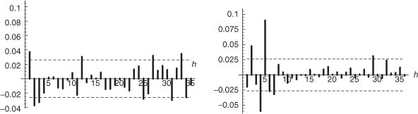
Figure 1.6 Sample autocorrelations ![]() (h) (h = 1, …, 36) of (a) the S&P 500 Index from January 3, 1979 to December 30, 2001, and (b) the squared Index. The Interval between the dashed lines (±1.96 /
(h) (h = 1, …, 36) of (a) the S&P 500 Index from January 3, 1979 to December 30, 2001, and (b) the squared Index. The Interval between the dashed lines (±1.96 /![]() , where n = 5804 is the sample length) should contain approximately 95% of a strong white noise.
, where n = 5804 is the sample length) should contain approximately 95% of a strong white noise.
1.9 (Stationary solutions of an AR(1))
Let (ηt)t![]()
![]() be an iid centered sequence with variance σ2 > 0, and let a ≠ 0. Consider the AR(1) equation
be an iid centered sequence with variance σ2 > 0, and let a ≠ 0. Consider the AR(1) equation
1. Show that for |a| < 1, the infinite sum
converges in quadratic mean and almost surely, and that it Is the unique stationary solution of (1.8).
2. For |a| = 1, show that no stationary solution exists.
3. For |a| > 1, show that
is the unique stationary solution of (1.8).
4. For |a| > 1, show that the causal representation
holds, where (![]() t)t
t)t![]()
![]() is a white noise.
is a white noise.
1.10 (Is the S&P 500 a white noise?)
Figure 1.6 displays the correlogram of the S&P 500 returns from January 3, 1979 to December 30, 2001, as well as the correlogram. of the squared returns. Is it reasonable to think that this index is a strong white noise or a weak white noise?
1.11 (Asymptotic covariance of sample autocovariances)
Justify the equivalence between (B.18) and (B.14) in the proof of the generalized Bartlett formula of Appendix B.2.
1.12 (Asymptotic independence between the ![]() (h) for a noise)
(h) for a noise)
Simplify the generalized Bartlett formulas (B.14) and (B.15) when X = ![]() is a pure white noise.
is a pure white noise.
In an autocorrelogram, consider the random number M of sample autocorrelations falling outside the significance region (at the level 95%, say), among the first m autocorrelations. How can the previous result be used to evaluate the variance of this number when the observed process is a white noise (satisfying the assumptions allowing (B.15) to be used)?
1.13 (An incorrect interpretation of autocorrelograms)
Some practitioners tend to be satisfied with an estimated model only if all sample autocorrelations fall within the 95% significance bands. Show, using Exercise 1.12, that based on 20 autocorrelations, say, this approach leads to wrongly rejecting a white noise with a very high probability.
1.14 (Computation of partial autocorrelations)
Use the algorithm in (B.7) – (B.9) to compute rX(l), rx(2) and rX (3) as a function of ρx(1), ρx(2) and ρX(3).
1.15 (Empirical application)
Download from http://fr.biz.yahoo.com//bourse/accueil.html for instance, a stock index such as the CAC 40. Draw the series of closing prices, the series of returns, the autocorrelation function of the returns, and that of the squared returns. Comment on these graphs.
1A stationary process (Xt) is said to be purely nondeterministic if and only if ![]() , where
, where ![]() x(n) denotes, in the Hilbert space of the real, centered, and square integrable variables, the subspace constituted by the limits of the linear combinations of the variables Xn−i, i ≥ 0. Thus, for a purely nondeterministic (or regular) process, the linear past, sufficiently far away in the past, is of no use in predicting future values. See Brockwell and Davis (1991, pp. 187–189) or Azencott and Dacunha-Castelle (1984) for more details.
x(n) denotes, in the Hilbert space of the real, centered, and square integrable variables, the subspace constituted by the limits of the linear combinations of the variables Xn−i, i ≥ 0. Thus, for a purely nondeterministic (or regular) process, the linear past, sufficiently far away in the past, is of no use in predicting future values. See Brockwell and Davis (1991, pp. 187–189) or Azencott and Dacunha-Castelle (1984) for more details.
2 In this representation, the equivalence class E(Xt|![]() x(t − 1)) is identified with a random variable.
x(t − 1)) is identified with a random variable.
3 In contrast, a process such that VarXt is constant is called (marginally) homoscedastic.
4 More precisely, for ![]() is a plausible realization of the |N(0, 1)| distribution.
is a plausible realization of the |N(0, 1)| distribution.
5 The CAC 40 index is a linear combination of a selection of 40 shares on the Paris Stock Exchange (CAC stands for ‘Cotations Assistées en Continu’).
6 There is no general agreement concerning the definition of this concept in the literature. Volatility sometimes refers to a conditional standard deviation, and sometimes to a conditional variance.
7 Note, however, that the volatility is also a random variable in GARCH-type processes.