Asymmetries
Classical GARCH models, studied in Parts I and II, rely on modeling the conditional variance as a linear function of the squared past innovations. The merits of this specification are its ability to reproduce several important characteristics of financial time series – succession of quiet and turbulent periods, autocorrelation of the squares but absence of autocorrelation of the returns, leptokurticity of the marginal distributions – and the fact that it is sufficiently simple to allow for an extended study of the probability and statistical properties.
From an empirical point of view, however, the classical GARCH modeling has an important drawback. Indeed, by construction, the conditional variance only depends on the modulus of the past variables: past positive and negative innovations have the same effect on the current volatility. This property is in contradiction to many empirical studies on series of stocks, showing a negative correlation between the squared current innovation and the past innovations: if the conditional distribution were symmetric in the past variables, such a correlation would be equal to zero. However, conditional asymmetry is a stylized fact: the volatility increase due to a price decrease is generally stronger than that resulting from a price increase of the same magnitude.
The symmetry property of standard GARCH models has the following interpretation in terms of autocorrelations. If the law of ηt is symmetric, and under the assumption that the GARCH process is second-order stationary, we have
because σt is an even function of the ∈t−i, i > 0 (see Exercise 10.1). Introducing the positive and negative components of ∈t,
it is easily seen that (10.1) holds if and only if
This characterization of the symmetry property in terms of autocovariances can be easily tested empirically, and is often rejected on financial series. As an example, for the log-returns series ∈t = log(pt / pt−1)) of the CAC 40 index presented in Chapter 1, we get the results shown in Table 10.1.
Table 10.1 Empirical autocorrelations (CAC 40 series, period 1988–1998).
*indicate autocorrelations which are statistically significant at the 5% level, using 1/n as an approximation of the autocorrelations variances, for n = 2385.
The absence of significant autocorrelations of the returns and the correlation of their modulus or squares, which constitute the basic properties motivating the introduction of GARCH models, are clearly shown for these data. But just as evident is the existence of an asymmetry in the impact of past innovations on the current volatility. More precisely, admitting that the process (∈t) is second-order stationary and can be decomposed as ∈t = σtηt, where (ηt) is an iid sequence and σt is a measurable, positive function of the past of ∈t, we have
where K > 0. For the CAC data, except when h = 1 for which the autocorrelation is not significant, the estimates of ![]() seem to be significantly negative.1 Thus
seem to be significantly negative.1 Thus
which can be interpreted as a higher impact of the past price decreases on the current volatility, compared to the past price increases of the same magnitude. This phenomenon, Cov(σt, ∈t−h) < 0, is known in the finance literature as the leverage effect:2 volatility tends to increase dramatically following bad news (that is, a fall in prices), and to increase moderately (or even to diminish) following good news.
The models we will consider In this chapter allow this asymmetry property to be Incorporated.
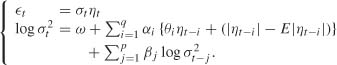
The following definition for the exponential GARCH (EGARCH) model mimics that given for the strong GARCH.
Definition 10.1 (EGARCH(p, q) process) Let (ηt) be an iid sequence such that E(ηt) = 0 and Var(ηt) = 1. Then (∈t) is said to be an exponential GARCH (EGARCH(p, q)) process if it satisfies an equation of the form
where
and ω, αi,βj, θ and ς are real numbers.
Remark 10.1 (On the EGARCH model)
1. The relation
shows that, In contrast to the classical GARCH, the volatility has a multiplicative dynamics. The positivity constraints on the coefficients can be avoided, because the logarithm can be of any sign.
2. According to the usual Interpretation, however, innovations of large modulus should increase volatility. This entails constraints on the coefficients: for instance, if log ![]() increases with |ηt−1|, the sign of ηt−1 being fixed, if and only if − ς < θ < ς. In the general case it suffices to Impose
increases with |ηt−1|, the sign of ηt−1 being fixed, if and only if − ς < θ < ς. In the general case it suffices to Impose
3. The asymmetry property is taken into account through the coefficient θ. For instance, let θ < 0 and log ![]() : if ηt−1 < 0 (that is, if ∈t−1 < 0), the variable log
: if ηt−1 < 0 (that is, if ∈t−1 < 0), the variable log ![]() will be larger than its mean ω, and it will be smaller if ∈t−1 > 0. Thus, we obtain the typical asymmetry property of financial time series.
will be larger than its mean ω, and it will be smaller if ∈t−1 > 0. Thus, we obtain the typical asymmetry property of financial time series.
4. Another difference from the classical GARCH is that the conditional variance is written as a function of the past standardized innovations (that is, divided by their conditional standard deviation), instead of the past innovations. In particular, log ![]() is a strong ARMA(p, q − q′) process, where q′ is the first Integer i such that αi ≠ 0, because (g(ηt)) is a strong white noise, with variance
is a strong ARMA(p, q − q′) process, where q′ is the first Integer i such that αi ≠ 0, because (g(ηt)) is a strong white noise, with variance
5. A formulation which is very close to the EGARCH is the Log-GARCH, defined by
where, obviously, one has to impose |ςi| < 1.
6. The specification (10.4) allows for sign effects, through ![]() , and for modulus effects through ς (|ηt−i| − E|ηt−i|). This obviously induces, however, at least in the case q = 1, an identifiabillty problem, which can be solved by setting ς = 1. Note also that, to allow different sign effects for the different lags, one could make θ depend on the lag index i, through the formulation
, and for modulus effects through ς (|ηt−i| − E|ηt−i|). This obviously induces, however, at least in the case q = 1, an identifiabillty problem, which can be solved by setting ς = 1. Note also that, to allow different sign effects for the different lags, one could make θ depend on the lag index i, through the formulation
As we have seen, specifications of the function g(·) that are different from (10.4) are possible, depending on the kind of empirical properties we are trying to mimic. The following result does not depend on the specification chosen for g(·). It is, however, assumed that Eg(ηt) exists and is equal to 0.
Theorem 10.1 (Stationarity of the EGARCH(p, q) process) Assume that g(ηt) is not almost surely equal to zero and that the polynomials ![]() and
and ![]() have no common root, with α(z) not identically null. Then, the EGARCH(p, q) model defined in (10.3) admits
have no common root, with α(z) not identically null. Then, the EGARCH(p, q) model defined in (10.3) admits
a strictly stationary and nonanticipative solution if and only if the roots of β(z) are outside the unit circle. This solution is such that E(log ![]() < ∞ whenever E(log
< ∞ whenever E(log ![]() < ∞ and Eg2(ηt) < ∞.
< ∞ and Eg2(ηt) < ∞.
If in addition,
where the λi are defined by ![]() , then (∈t) is a white noise with variance
, then (∈t) is a white noise with variance
where ω* = ω/β(1) and gη(x) = E[exp{xg(ηt)}].
Proof. We have log ![]() = log
= log ![]() + log
+ log ![]() . Because log
. Because log ![]() is the solution of an ARMA(p, q − 1) model, with AR polynomial β, the assumptions made on the lag polynomials are necessary and sufficient to express, in a unique way, log
is the solution of an ARMA(p, q − 1) model, with AR polynomial β, the assumptions made on the lag polynomials are necessary and sufficient to express, in a unique way, log ![]() as an infinite-order moving average:
as an infinite-order moving average:
It follows that the processes (log ![]() and (log
and (log ![]() ) are strictly stationary. The process (log
) are strictly stationary. The process (log ![]() ) is second-order stationary and, under the assumption is E(log
) is second-order stationary and, under the assumption is E(log ![]() < ∞, so is (log
< ∞, so is (log ![]() ). Moreover, using the previous expansion,
). Moreover, using the previous expansion,
Using the fact that the process g(ηt) is iid, we get the desired result on the expectation of (![]() ) (Exercise 10.4).
) (Exercise 10.4).
Remark 10.2
1. When βj = 0 for j = 1,…, p (EARCH(q) model), the coefficients λi cancel for i > q. Hence, condition (10.6) is always satisfied, provided that E exp{|αig(ηt)|} < ∞, for i = 1, …,q. If the tails of the distribution of ηt are not too heavy (the condition fails for the Student t distributions and specification (10.4)), an EARCH(q) process is then stationary, in both the strict and second-order senses, whatever the values of the coefficients αi.
2. When ηt is ![]() (0, 1) distributed, and if g(·) is such that (10.4) holds, one can verify (Exercise 10.5) that
(0, 1) distributed, and if g(·) is such that (10.4) holds, one can verify (Exercise 10.5) that
Since the λi are obtained from the inversion of the polynomial β(·), they decrease exponentially fast to zero. It is then easy to check that (10.6) holds true in this case, without any supplementary assumption on the model coefficients. The strict and second-order stationarity conditions thus coincide, contrary to what happened In the standard GARCH case. To compute the second-order moments, classical integration calculus shows that
where Ф denotes the cumulative distribution function of the ![]() (0, 1).
(0, 1).
Theorem 10.2 (Moments of the EGARCH(p, q) process) Let m be a positive integer. Under the conditions of Theorem 10.1 and if
(![]() ) admits a moment of order m given by
) admits a moment of order m given by
Proof. The result straightforwardly follows from (10.7) and Exercise 10.4.
The previous computation shows that in the Gaussian case, moments exist at any order. This shows that the leptokurticity property may be more difficult to capture with EGARCH than with standard GARCH models.
Assuming that E(log ![]() )2 < ∞, the autocorrelation structure of the process (log
)2 < ∞, the autocorrelation structure of the process (log ![]() ) can be derived by taking advantage of the ARMA form of the dynamics of log
) can be derived by taking advantage of the ARMA form of the dynamics of log ![]() . Indeed, replacing the terms in
. Indeed, replacing the terms in ![]() by
by ![]() , we get
, we get
Let
One can easily verify that (υt) has finite variance. Since υt only depends on a finite number r (r = max(p, q)) of past values of ηt, it is clear that Cov(υt, υt−k) = 0 for k > r. It follows that (υt) is an MA(r) process (with intercept) and thus that (log ![]() ) is an ARMA(p, r) process. This result is analogous to that obtained for the classical GARCH models, for which an ARMA(r, p) representation was exhibited for
) is an ARMA(p, r) process. This result is analogous to that obtained for the classical GARCH models, for which an ARMA(r, p) representation was exhibited for ![]() . Apart from the inversion of the integers r and p, it is important to note that the noise of the ARMA equation of a GARCH is the strong innovation of the square, whereas the noise involved in the ARMA equation of an EGARCH is generally not the strong innovation of log
. Apart from the inversion of the integers r and p, it is important to note that the noise of the ARMA equation of a GARCH is the strong innovation of the square, whereas the noise involved in the ARMA equation of an EGARCH is generally not the strong innovation of log ![]() . Under this limitation, the ARMA representation can be used to identify the orders p and q and to estimate the parameters βj and αi (although the latter do not explicitly appear In the representation).
. Under this limitation, the ARMA representation can be used to identify the orders p and q and to estimate the parameters βj and αi (although the latter do not explicitly appear In the representation).
The autocorrelations of (![]() ) can be obtained from formula (10.7). Provided the moments exist we have, for h > 0,
) can be obtained from formula (10.7). Provided the moments exist we have, for h > 0,
the first product being replaced by 1 if h = 1. For h > 0, this leads to
A natural way to introduce asymmetry is to specify the conditional variance as a function of the positive and negative parts of the past innovations. Recall that
and note that ![]() . The threshold GARCH (TGARCH) class of models introduces a threshold effect into the volatility.
. The threshold GARCH (TGARCH) class of models introduces a threshold effect into the volatility.
Definition 10.2 (TGARCH(p, q) process) Let (ηt) be an iid sequence of random variables such that E(ηt) = 0 and Var(ηt) = 1. Then (ηt) is called a threshold GARCH(p, q) process if it satisfies an equation of the form
where ω, αi+, αi,− and βi are real numbers.
Remark 103 (On the TGARCH model)
1. Under the constraints
the variable σt is always strictly positive and represents the conditional standard deviation of ∈t. In general, the conditional standard deviation of ∈t is |σt|: imposing the positivity of σt is not required (contrary to the classical GARCH models, based on the specification of ![]() ).
).
2. The GJR-GARCH model (named for Glosten, Jagannathan and Runkle, 1993) is a variant, defined by
which corresponds to squaring the variables involved in the second equation of (10.9).
3. Through the coefficients αi+ and αi−, the current volatility depends on both the modulus and the sign of past returns. The model is flexible, allowing the lags i of the past returns to display different asymmetries. Note also that this class contains, as special cases, models displaying no asymmetry, whose properties are very similar to those of the standard GARCH. Such models are obtained for αi+ = αi− := αi (i = 1, …, q) and take the form
(since ![]() ). This specification is called absolute value GARCH (AVGARCH). Whether it is preferable to model the conditional variance or the conditional standard deviation is an open issue. However, it must be noted that for regression models with
). This specification is called absolute value GARCH (AVGARCH). Whether it is preferable to model the conditional variance or the conditional standard deviation is an open issue. However, it must be noted that for regression models with
non-Gaussian and heteroscedastic errors, one can show that estimators of the noise variance based on the absolute residuals are more efficient than those based on the squared residuals (see Davidian and Carroll, 1987).
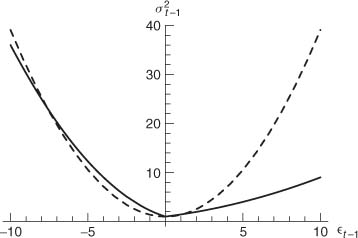
Figure 10.1 depicts the major difference between GARCH and TGARCH models. The so-called ‘news impact curves’ display the impact of the innovations at time t − 1 on the volatility at time t, for first-order models. In this figure, the coefficients have been chosen in such a way that the marginal variances of ∈t in the two models coincide. In this TARCH example, in accordance with the properties of financial time series, negative past values of ∈t−1 have more impact on the volatility than positive values of the same magnitude. The impact is, of course, symmetrical in the ARCH case.
TGARCH models display linearity properties similar to those encountered for the GARCH. Under the positivity constraints (10.10), we have
which allows us to write the conditional standard deviation in the form
where ![]() . The dynamics of σt is thus given by a random coefficient autoregressive model.
. The dynamics of σt is thus given by a random coefficient autoregressive model.
Stationarity of the TGARCH(1,1) Model
The study of the stationarity properties of the TGARCH(1, 1) model is based on (10.12) and follows from similar arguments to the GARCH(1, 1) case. The strict stationarity condition is written as
Figure 10.1 News impact curves for the ARCH(1) model, ![]() (dashed line), and TARCH(l) model,
(dashed line), and TARCH(l) model, ![]() (solid line).
(solid line).
In particular, for the TARCH(l) model (β1 = 0) we have
Hence, if the distribution of (ηt) is symmetric the expectation of the two indicator variables is equal to 1/2 and the strict stationarity condition reduces to
Exercise 10.8 shows that the second-order stationarity condition is
This condition can be made explicit in terms of the first two moments of ![]() and
and ![]() . For instance, if ηt is
. For instance, if ηt is ![]() (0, 1) distributed, we get
(0, 1) distributed, we get
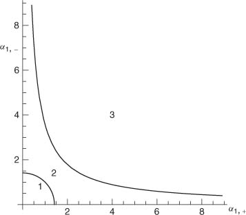
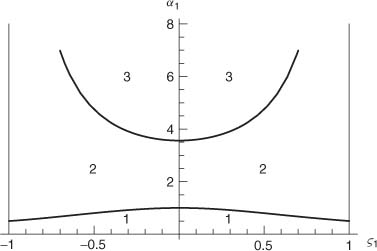
Of course, the second-order stationarity condition is more restrictive than the strict stationarity condition (see Figure 10.2).
Under the second-order stationarity condition, it is easily seen that the property of symmetry (10.1) is generally violated. For instance if the distribution of ηt is symmetric, we have, for the TARCH(l) model:
whenever α1,+ ≠ α1,−.
Figure 10.2 Stationarity regions for the TARCH(l) model with ηt ~ ![]() (0, 1): 1, second-order stationarity; 1 and 2, strict stationarity; 3, nonstationarity.
(0, 1): 1, second-order stationarity; 1 and 2, strict stationarity; 3, nonstationarity.
Strict Stationarlty of the TGARCH(p, q) Model
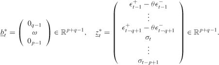
The study of the general ease relies on a representation analogous to (2.16), obtained by replacing, in the vector ![]() the variables
the variables ![]() by
by ![]() the
the ![]() by σt−i, and by an adequate modification of
by σt−i, and by an adequate modification of ![]() and At. Specifically, using (10.11), we get
and At. Specifically, using (10.11), we get
where
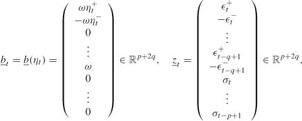
and
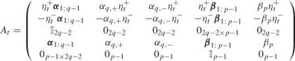
is a matrix of size (p + 2q) × (p + 2q),
The following result is analogous to that obtained for the strict stationarlty of the GARCH(p, q).
Theorem 10.3 (Strict stationarlty of the TGARCH(p,q) model) A necessary and sufficient condition for the existence of a strictly stationary and nonanticipative solution of the TGARCH(p, q) model (10.9)–(10.10) is that γ < 0, where γ is the top Lyapunov exponent of the sequence {At, t ∈ ![]() } defined by (10.17).
} defined by (10.17).
This stationary and nonanticipative solution, when γ < 0, is unique and ergodic.
Proof. The sufficient part of the proof of Theorem 2.4 can be straightforwardly adapted. As for the necessary part, note that the coefficients of the matrices At, ![]() and
and ![]() are positive. This allows us to show, as was done previously, that
are positive. This allows us to show, as was done previously, that ![]() tends to 0 almost surely when k → ∞. But since
tends to 0 almost surely when k → ∞. But since ![]() , using the positivity, we have
, using the positivity, we have
It follows that ![]() a.s. for i = 1,… 2q + 1 by induction, as in the GARCH case.
a.s. for i = 1,… 2q + 1 by induction, as in the GARCH case.
Numerical evaluation, by means of simulation, of the Lyapunov coefficient γ can be time-consuming because of the large size of the matrices At. A condition involving matrices of smaller dimensions can sometimes be obtained. Suppose that the asymmetric effects have a factorization the form ![]() for all lags i=l,…,q. In this constrained model, the asymmetry is summarized by only one parameter θ≠ 1, the case θ > 1 giving more importance to the negative returns.
for all lags i=l,…,q. In this constrained model, the asymmetry is summarized by only one parameter θ≠ 1, the case θ > 1 giving more importance to the negative returns.
Theorem 10.4 (Strict stationarity of the constrained TGARCH (p, q) model) A necessary and sufficient condition for the existence of a strictly stationary and nonanticipative solution of the TGARCH(p,q) model (10.9), in which the coefficients ω, αi,− and αi,+ satisfy the positivity conditions (10.10) and the q − 1 constraints
is that γ* < 0, where γ* is the top Lyapunov exponent of the sequence of (p + q − 1) × (p + q − 1) matrices ![]() defined by
defined by
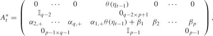
where ![]() . This stationary and nonanticipative solution, when γ* < 0, is unique and ergodic.
. This stationary and nonanticipative solution, when γ* < 0, is unique and ergodic.
Proof. If the constrained TGARCH model admits a stationary solution (σt, ∈t), then a stationary solution exists for the model
where
Conversely, if (10.19) admits a stationary solution, then the constrained TGARCH model admits the stationary solution (σt,∈t) defined by ![]() (the qth component of
(the qth component of ![]() ) and ∈t =σtηt. Thus the constrained TGARCH model admits a strictly stationary solution if and only if model (10.19) has a strictly stationary solution. It can be seen that
) and ∈t =σtηt. Thus the constrained TGARCH model admits a strictly stationary solution if and only if model (10.19) has a strictly stationary solution. It can be seen that ![]() implies
implies ![]() for i − 1,…, p + q − 1, using the independence of the matrices in the product
for i − 1,…, p + q − 1, using the independence of the matrices in the product ![]() and noting that, in the case where θ(ηt) is not almost surely equal to zero, the qth component of
and noting that, in the case where θ(ηt) is not almost surely equal to zero, the qth component of ![]() the first and (q + l)th components of
the first and (q + l)th components of ![]() the second and (q + 2)th components of
the second and (q + 2)th components of ![]() , etc., are strictly positive with nonzero probability. In the case where θ(ηt) = 0, the first q − 1 rows of
, etc., are strictly positive with nonzero probability. In the case where θ(ηt) = 0, the first q − 1 rows of ![]() are null, which obviously shows that
are null, which obviously shows that ![]() for i = 1,…, q − 1. For i = q,…, p + q − 1, the argument used in the case θ(ηt) ≠ 0 remains valid. The rest of the proof is similar to that of Theorem 2.4.
for i = 1,…, q − 1. For i = q,…, p + q − 1, the argument used in the case θ(ηt) ≠ 0 remains valid. The rest of the proof is similar to that of Theorem 2.4.
mth-Order Stationarity of the TGARCH(p, q) Model
Contrary to the standard GARCH model, the odd-order moments are not more difficult to obtain than the even-order ones for a TGARCH model. The existence condition for such moments is provided by the following theorem.
Theorem 10.5 (mth-order stationarity) Let m be a positive integer. Suppose that E(|ηt|m) < ∞. ![]() where At is defined by (10.16). If the spectral radius
where At is defined by (10.16). If the spectral radius
then, for any t ∈ ![]() , the infinite sum (
, the infinite sum (![]() ) is a strictly stationary solution of (10.16) which converges in Lm and the process (∈t), defined by
) is a strictly stationary solution of (10.16) which converges in Lm and the process (∈t), defined by ![]() is a strictly stationary solution of the TGARCH(p, q) model defined by (10.9), and admits moments up to order m.
is a strictly stationary solution of the TGARCH(p, q) model defined by (10.9), and admits moments up to order m.
Conversely, if ρ(A(m)) ≥ 1, there exists no strictly stationary solution (∈t) of (10.9) satisfying the positivity conditions (10.10) and the moment condition E(|∈t|m) < ∞.
The proof of this theorem is identical to that of Theorem 2.9.
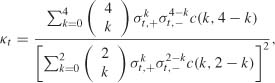
Kurtosis of the TGARCH(1,1) Model
For the TGARCH(1, 1) model with positive coefficients, the condition for the existence of E|∈t|m can be obtained directly. Using the representation
we find that ![]() exists and satisfies
exists and satisfies
if and only if
If this condition is satisfied for m = 4, then the kurtosis coefficient exists. Moreover, If ∈t ~ ![]() (0, 1) we get
(0, 1) we get
and, using the notation ρi = Eρi(ηt), the moments can be computed successively as
Many moments of the TGARCH(1, 1) can be obtained similarly, such as the autocorrelations of the absolute values (Exercise 10.9) and squares, but the calculations can be tedious.
10.3 Asymmetric Power GARCH Model
The following class is very general and contains the standard GARCH, the TGARCH, and the Log-GARCH.
Definition 10.3 (APARCH(p q) process) Let (ηt) be a sequence of iid variables such that E(ηt) = 0 and Var(ηt) = 1. The process (∈t) is called an asymmetric power GARCH(p, q)) if it satisfies an equation of the form
where ω > 0, δ > 0, αi≥0,βi ≥ 0 and |ςi| Ⅴ 1.
Remark 10.4 (On the APARCH model)
1. The standard GARCH (p, q) is obtained for δ = 2 and ς1 = … = ςq = 0.
2. To study the role of the parameter ςi, let us consider the simplest case, the asymmetric ARCH(l) model. We have
Hence, the choice of ςi > 0 ensures that negative innovations have more impact on the current volatility than positive ones of the same modulus. Similarly, for more complex APARCH models, the constraint ςi ≥ 0 is a natural way to capture the typical asymmetric property of financial series.
3. Since
|ςi| ≤ 1 is a nonrestrictive identifiability constraint.
4. If δ = 1, the model reduces to the TGARCH model. Using ![]() , one can interpret the Log-GARCH model as the limit of the APARCH model when δ → 0. The novelty of the APARCH model is in the introduction of the parameter δ. Note that
, one can interpret the Log-GARCH model as the limit of the APARCH model when δ → 0. The novelty of the APARCH model is in the introduction of the parameter δ. Note that
autocorrelations of the absolute returns are often larger than autocorrelations of the squares. The introduction of the power δ increases the flexibility of GARCH-type models, and allows the a priori selection of an arbitrary power to be avoided.
Noting that ![]() , one can write
, one can write
where
for i = 1,…, max {p, q}.
Stationarity of the APARCH(1,1) Model
Relation (10.23) is an extension of (2.6) which allows us to obtain the statlonarity conditions, as in the classical GARCH(1, 1) case. The necessary and sufficient strict statlonarity condition is thus
For the APARCH(1, 0) model, we have
showing that, if the distribution of (ηt) symmetric, the strict statlonarity condition reduces to
Note that in the limit case where |ς1| = 1, the model is strictly stationary for any value of α1, as might be expected. Under condition (10.24), the strictly stationary solution is given by
Assuming E|ηt|δ < ∞, the condition for the existence of ![]() (and of
(and of ![]() ) is
) is
which reduces to
when the distribution of (ηt) symmetric, with
when ηt is Gaussian (Г denoting the Euler gamma function). Figure 10.3 shows the strict and second-order statlonarity regions of the APARCH(1, 0) model when ηt is Gaussian.
Figure 10.3 Stationarity regions for the APARCH(1,0) model with ηt ~ ![]() (0,1): 1, second-order stationarity; 1 and 2, strict stationarity; 3, nonstationarity.
(0,1): 1, second-order stationarity; 1 and 2, strict stationarity; 3, nonstationarity.
Obviously, if δ ≥ 2 condition (10.25) is sufficient (but not necessary) for the existence of a strictly stationary and second-order stationary solution to the APARCH(1, 1) model. If δ ≤ 2, condition (10.25) is necessary (but not sufficient) for the existence of a second-order stationary solution.
10.4 Other Asymmetric GARCH Models
Among other asymmetric GARCH models, which we will not study in detail, let us mention the qualitative threshold ARCH (QTARCH) model, and the quadratic GARCH model (QGARCH or GQARCH), generalizing Example 4.2 in Chapter 4. The first-order model of this class, the QGARCH(1, 1), is defined by
where ηt is a strong white noise with unit variance.
Remark 10.5 (On the QGARCH(1,1) model)
1. The function x ↦ ax2 + ςx has its minimum at x = − ς/2α, and this minimum is − ς2/4α. A condition ensuring the positivity of ![]() is thus ω> −ς2/4α. This can also be seen by writing
is thus ω> −ς2/4α. This can also be seen by writing
2. The condition
is clearly necessary for the existence of a nonanticipative and second-order stationary solution, but it seems difficult to prove that this condition suffices for the existence of a solution. Equation (10.26) cannot be easily expanded because of the presence of ![]() and ∈t−1 = σt−1ηt−1. It is therefore not possible to obtain an explicit solution as a function of the ηt−i. This makes QGARCH models much less tractable than the asymmetric models studied in this chapter.
and ∈t−1 = σt−1ηt−1. It is therefore not possible to obtain an explicit solution as a function of the ηt−i. This makes QGARCH models much less tractable than the asymmetric models studied in this chapter.
3. The asymmetric effect is taken into account through the coefficient ς. A negative coefficient entails that negative returns have a bigger impact on the volatility of the next period than positive ones. A small price increase, such that the return is less than − ς/2α with ς > 0, can even produce less volatility than a zero return. This is a distinctive feature of this model, compared to the EGARCH, TGARCH or GJR-GARCH for which, by appropriately constraining the parameters, the volatility at time t is minimal in the absence of price movement at time t − 1.
Many other asymmetric GARCH models have been introduced. Complex asymmetric responses to past values may be considered. For instance, in the model
asymmetry is only present for large innovations (whose amplitude is larger than the threshold γ).
10.5 A GARCH Model with Contemporaneous Conditional Asymmetry
A common feature of the GARCH models studied up to now is the decomposition
where σt is a positive variable and (ηt) is an iid process. The various models differ by the specification of σt as a measurable function of the ∈t−i for i > 0. This type of formulation implies several important restrictions:
(i) The process (∈t) is a martingale difference.
(ii) The positive and negative parts of ∈t have the same volatility, up to a multiplicative factor.
(iii) The kurtosis and skewness of the conditional distribution of ∈t are constant.
Property (ii) is an immediate consequence of the equalities in (10.11). Property (iii) expresses the fact that the conditional law of ∈t has the same ‘shape’ (symmetric or asymmetric, unimodal or polymodal, with or without heavy tails) as the law of ηt.
It can be shown empirically that these properties are generally not satisfied by financial time series. Estimated kurtosis and skewness coefficients of the conditional distribution often present large variations in time. Moreover, property (i) implies that Cov(∈t,zt−1) = 0, for any variable zt−1 ∈ L2 which is a measurable function of the past of ∈t. In particular, one must have
or, equivalently,
We emphasize the difference between (10.27) and the characterization (10.2) of the asymmetry studied previously. When (10.27) does not hold, one can speak of contemporaneous asymmetry since the variables ![]() and
and ![]() , of the current date, do not have the same conditional distribution. For the CAC index series, Table 10.2 completes Table 10.1, by providing the cross empirical autocorrelations of the positive and negative parts of the returns.
, of the current date, do not have the same conditional distribution. For the CAC index series, Table 10.2 completes Table 10.1, by providing the cross empirical autocorrelations of the positive and negative parts of the returns.
Table 10.2 Empirical autocorrelations (CAC 40, for the period 1988–1998).
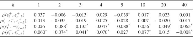
*indicate parameters that are statistically significant at the level 5%, using 1/n as an approximation for the autocorrelations variance, for n = 2385.
Without carrying out a formal test, comparison of rows 1 and 3 (or 2 and 4) shows that the leverage effect is present, whereas comparison of rows 3 and 4 shows that property (10.28) does not hold.
A class of GARCH-type models allowing the two kinds of asymmetry is defined as follows. Let
where {ρt} is centered, ρt is independent of σt+ and σt−, and
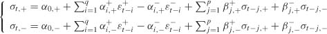
where ![]() . Without loss of generality, it can be assumed that
. Without loss of generality, it can be assumed that ![]() .
.
As an immediate consequence of the positivity of σt+ and σt−, we obtain
which will be crucial for the study of this model.
Thus, σt+ and σt− can be interpreted as the volatilities of the positive and negative parts of the noise (up to a multiplicative constant, since we did not specify the variances of ![]() and
and ![]() ). In general, the nonanticipative solution of this model, when it exists, is not a martingale difference because
). In general, the nonanticipative solution of this model, when it exists, is not a martingale difference because
An exception is of course the situation where the parameters of the dynamics of σt,+ and σt,− coincide, in which case we obtain model (10.9).
A simple computation shows that the kurtosis coefficient of the conditional law of ∈t is given by
where ![]() , provided that E(
, provided that E(![]() ) < ∞. A similar computation can be done for the conditional skewness, showing that the shape of the conditional distribution varies in time, in a more important way than for classical GARCH models.
) < ∞. A similar computation can be done for the conditional skewness, showing that the shape of the conditional distribution varies in time, in a more important way than for classical GARCH models.
Methods analogous to those developed for the other GARCH models allow us to obtain existence conditions for the stationary and nonanticipative solutions (references are given at the end of the chapter). In contrast to the GARCH models analyzed previously, the stationary solution (∈t) is not always a white noise.
10.6 Empirical Comparisons of Asymmetric GARCH Formulations
We will restrict ourselves to the simplest versions of the GARCH introduced in this chapter, and consider their fit to the series of CAC 40 index returns, rt, over the period 1988–1998 consisting of 2385 values.
Descriptive Statistics
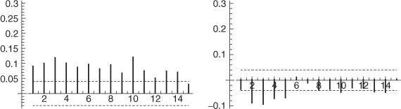
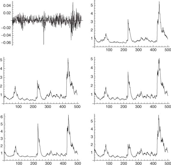
Figure 10.4 displays the first 500 values of the series. The volatility clustering phenomenon is clearly evident. The correlograms in Figure 10.5 indicate absence of autocorrelation. However, squared returns present significant autocorrelations, which is another sign that the returns are not independent. Ljung-Box portmanteau tests, such as those available in SAS (see Table 10.3; Chapter 5 gives more details on these tests), confirm the visual analysis provided by the correlograms. The left-hand graph of Figure 10.6, compared to the right-hand graph of Figure 10.5, seems to indicate that the absolute returns are slightly more strongly correlated than the squares. The right-hand graph of Figure 10.6 displays empirical correlations between the series |rt| and rt−h. It can be seen that these correlations are negative, which implies the presence of leverage effects (more accentuated, apparently, for lags 2 and 3 than for lag 1).
Figure 10.4 The first 500 values of the CAC 40 index (left) and of the squared index (right).
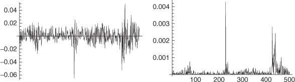
Figure 10.5 Correlograms of the CAC 40 index (left) and the squared index (right). Dashed lines correspond to ±1.96/![]() .
.
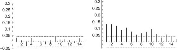
Table 10.3 Portmanteau test of the white noise hypothesis for the CAC 40 series (upper panel) and for the squared index (lower panel).
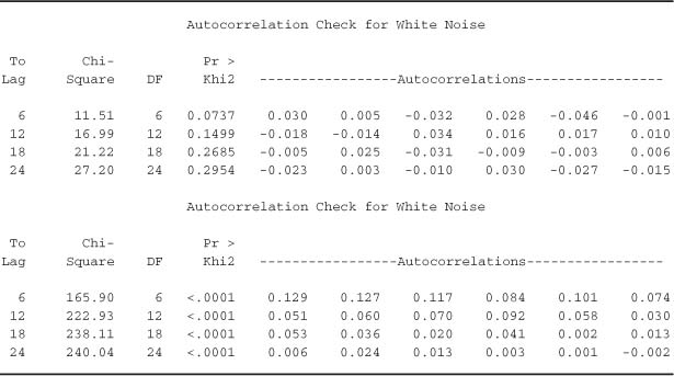
Figure 10.6 Correlogram ![]() of the absolute CAC 40 returns (left) and cross correlograms
of the absolute CAC 40 returns (left) and cross correlograms ![]() measuring the leverage effects (right).
measuring the leverage effects (right).
Fit by Symmetric and Asymmetric GARCH Models
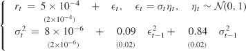
We will consider the classical GARCH(1, 1) model and the simplest asymmetric models (which are the most widely used). Using the AUTOREG and MODEL procedures of SAS, the estimated models are:
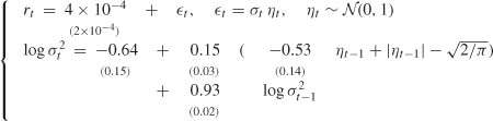
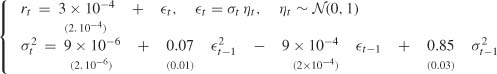
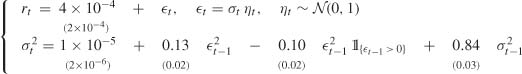
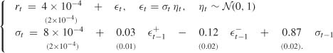
GARCH(1, 1) model
QGARCH(1, 1) model
GJR-GARCH(1, 1) model
TGARCH(1, 1) model
Interpretation of the Estimated Coefficients
Note that all the estimated models are stationary. The standard GARCH(1, 1) admits a fourth-order moment since, in view of the computation on page 45, we have 3α2 + 3β2 + 2αβ < 1. It is thus possible to compute the variance and kurtosis in this estimated model (which are respectively equal to 1.3 × 10⁻⁴ and 3.49 for the standard GARCH(1, 1)). Given the ARMA(1, 1) representation for ![]() , we have
, we have ![]() for any h > 1. Since
for any h > 1. Since ![]() +
+ ![]() = 0.09 + 0.84 is close to 1, the decay of ρ∈2(h) to zero will be slow when h → ∞, which can be interpreted as a sign of strong persistence of shocks.3
= 0.09 + 0.84 is close to 1, the decay of ρ∈2(h) to zero will be slow when h → ∞, which can be interpreted as a sign of strong persistence of shocks.3
Note that in the EGARCH model the parameter θ = −0.53 is negative, implying the presence of the leverage effect. A similar interpretation can be given to the negative sign of the coefficient of ∈t−1 in the QGARCH model, and to that of ![]() in the GJR-GARCH model. In the TGARCH model, the leverage effect is present since α1,− > α1,+ > 0.
in the GJR-GARCH model. In the TGARCH model, the leverage effect is present since α1,− > α1,+ > 0.
The TGARCH model seems easier to interpret than the other asymmetric models. The volatility (that is, the conditional standard deviation) is the sum of four terms. The first is the intercept ω = 8 × 10⁻⁴. The term ω/(1 −β1) = 0.006 can be interpreted as a ‘minimal volatility’, obtained by assuming that all the innovations are equal to zero. The next two terms represent the impact of the last observation, distinguishing the sign of this observation, on the current volatility. In the
Table 10.4 Likelihoods of the different models for the CAC 40 series.

estimated model, the impact of a positive value is 3.5 times less than that of a negative one. The last coefficient measures the importance of the last volatility. Even in absence of news, the decay of the volatility is slow because the coefficient β1 = 0.87 is rather close to 1.
Likelihood Comparisons
Table 10.4 gives the log-likelihood, log Ln, of the observations for the different models. One cannot directly compare the log-likelihood of the standard GARCH(1, 1) model, which has one parameter less, with that of the other models, but the log-likelihoods of the asymmetric models, which all have five parameters, can be compared. The largest likelihood is observed for the GJR threshold model, but, the difference being very slight, it is not clear that this model is really superior to the others.
Resemblances between the Estimated Volatilities
Figure 10.7 shows that the estimated volatilities for the five models are very similar. It follows that the different specifications produce very similar prediction intervals (see Figure 10.8).
Distances between Estimated Models
Differences can, however, be discerned between the various specifications. Table 10.5 gives an insight into the distances between the estimated volatilities for the different models. From this point of view, the TGARCH and EGARCH models are very close, and are also the most distant from the standard GARCH. The QGARCH model is the closest to the standard GARCH. Rather surprisingly, the TGARCH and GJR-GARCH models appear quite different. Indeed, the GJR-GARCH is a threshold model for the conditional variance and the TGARCH is a similar model for the conditional standard deviation.
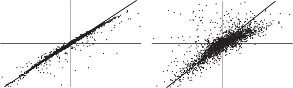
Figure 10.9 confirms the results of Table 10.5. The left-hand scatterplot shows
and the right-hand one
The left-hand graph shows that the difference between the estimated volatilities of the TGARCH and the standard GARCH, denoted by ![]() is alwavs very close to the difference between the estimated volatilities of the EGARCH and the standard GARCH, denoted by
is alwavs very close to the difference between the estimated volatilities of the EGARCH and the standard GARCH, denoted by ![]() (the difference from the standard GARCH is introduced to make the graphs more readable). The right-hand graph shows much more important differences between the TGARCH and GJR-GARCH specifications.
(the difference from the standard GARCH is introduced to make the graphs more readable). The right-hand graph shows much more important differences between the TGARCH and GJR-GARCH specifications.
Comparison between Implied and Sample Values of the Persistence and of the Leverage Effect
We now wish to compare, for the different models, the theoretical autocorrelations ρ(|rt|,|rt−h|) and ρ(|rt|,rt−h) to the empirical ones. The theoretical autocorrelations being difficult - if not
Figure 10.7 From left to right and top to bottom, graph of the first 500 values of the CAC 40 index and estimated volatilities (×104) for the GARCH(1, 1), EGARCH(1, 1), QGARCH(1, 1), GJR-GARCH(1, 1) and TGARCH(1, 1) models.
impossible - to obtain analytically, we used simulations of the estimated model to approximate these theoretical autocorrelations by their empirical counterparts. The length of the simulations, 50 000, seemed sufficient to obtain good accuracy (this was confirmed by comparing the empirical and theoretical values when the latter were available).
Figure 10.10 shows satisfactory results for the standard GARCH model, as far as the autocorrelations of absolute values are concerned. Of course, this model is not able to reproduce the correlations induced by the leverage effect. Such autocorrelations are adequately reproduced by the TARCH model, as can be seen from the top and bottom right panels. The autocorrelations for the other asymmetric models are not reproduced here but are very similar to those of the TARCH. The negative correlations between rt and the rt−h appear similar to the empirical ones.
Implied and Empirical Kurtosis
Table 10.6 shows that the theoretical variances obtained from the estimated models are close to the observed variance of the CAC 40 index. In contrast, the estimated kurtosis values are all much below the observed value.
Figure 10.8 Returns rt of the CAC 40 index (solid lines) and confidence intervals ![]() (dotted lines), where
(dotted lines), where ![]() is the empirical mean of the returns over the whole period 1988–1998 and σt is the estimated volatility in the standard GARCH(1, 1) model (left) and in the EGARCH(1, 1) model (right).
is the empirical mean of the returns over the whole period 1988–1998 and σt is the estimated volatility in the standard GARCH(1, 1) model (left) and in the EGARCH(1, 1) model (right).
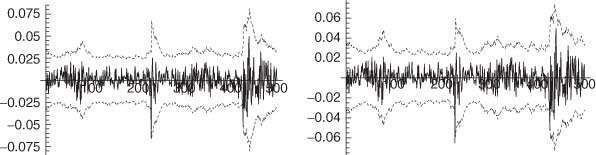
Table 10.5 Means of the squared differences between the estimated volatilities (× 1010).
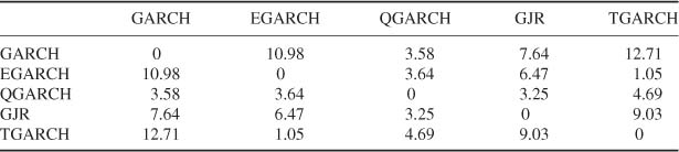
Figure 10.9 Comparison of the estimated volatilities of the EGARCH and TARCH models (left), and of the TGARCH and GJR-GARCH models (right). The estimated volatilities are close when the scatterplot is elongated (see text).
In all these five models, the conditional distribution of the returns is assumed to be ![]() (0, 1). This choice may be inadequate, which could explain the discrepancy between the estimated theoretical and the empirical kurtosis. Moreover, the normality assumption is clearly rejected by statistical tests, such as the Kolmogorov-Smirnov test, applied to the standardized returns. A leptokurtic distribution is observed for those standardized returns.
(0, 1). This choice may be inadequate, which could explain the discrepancy between the estimated theoretical and the empirical kurtosis. Moreover, the normality assumption is clearly rejected by statistical tests, such as the Kolmogorov-Smirnov test, applied to the standardized returns. A leptokurtic distribution is observed for those standardized returns.
Table 10.7 reveals a large number of returns outside the interval ![]() , whatever the specification used for
, whatever the specification used for ![]() . If the conditional law were Gaussian and if the conditional variance were
. If the conditional law were Gaussian and if the conditional variance were
Figure 10.10 Correlogram h ↦ ρ(|rt|,|rt−h|) of the absolute values (left) and cross correlogram h ↦ ρ(|rt|,rt−h) measuring the leverage effect (right), for the CAC 40 series (top), for the standard GARCH (middle), and for the TGARCH (bottom) estimated on the CAC 40 series.
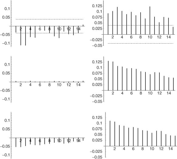
Table 10.6 Variance (× 104) and kurtosis of the CAC 40 index and of simulations of length 50 000 of the five estimated models.
correctly specified, the probability of one return falling outside the interval would be 2{1 − B(3)} = 0.0027, which would correspond to an average of 6 values out of 2385.
Asymmetric GARCH Models with Non-Gaussian Innovations
To take into account the leptokurtic shape of the residuals distribution, we re-estimated the five GARCH models with a Student t distribution - whose parameter is estimated - for ηt.
Table 10.7 Number of CAC returns outside the limits ![]() (THEO being the theoretical number when the conditional distribution is
(THEO being the theoretical number when the conditional distribution is ![]() .
.

Table 10.8 Means of the squares of the differences between the estimated volatilities (× 1010) for the models with Student innovations and the TGARCH model with Gaussian innovations (model (1034) denoted TGARCHN).
For instance, the new estimated TGARCH model is
It can be seen that the estimated volatility is quite different from that obtained with the normal distribution (see Table 10.8).
Model with Interventions
Analysis of the residuals show that the values observed at times t = 228, 682 and 845 are scarcely compatible with the selected model. There are two ways to address this issue: one could either research a new specification that makes those values compatible with the model, or treat these three values as outliers for the selected model.
In the first case, one could replace the ![]() (0, 1) distribution of the noise ηt with a more appropriate (leptokurtic) one. The first difficulty with this is that no distribution is evident for these data (it is clear that distributions of Student t or generalized error type would not provide good approximations of the distribution of the standardized residuals). The second difficulty is that changing the distribution might considerably enlarge the confidence intervals. Take the example of a 99% confidence interval at horizon 1. The initial interval
(0, 1) distribution of the noise ηt with a more appropriate (leptokurtic) one. The first difficulty with this is that no distribution is evident for these data (it is clear that distributions of Student t or generalized error type would not provide good approximations of the distribution of the standardized residuals). The second difficulty is that changing the distribution might considerably enlarge the confidence intervals. Take the example of a 99% confidence interval at horizon 1. The initial interval ![]() simply becomes the dilated interval
simply becomes the dilated interval ![]() with t0.995 ≫ 2.57, provided that the estimates
with t0.995 ≫ 2.57, provided that the estimates ![]() are not much affected by the change of conditional distribution. Even if the new interval does contain 99% of returns, there is a good chance that it will be excessively large for most of the data.
are not much affected by the change of conditional distribution. Even if the new interval does contain 99% of returns, there is a good chance that it will be excessively large for most of the data.
So for this first case we should ideally change the prediction formula for σt so that the estimated volatility is larger for the three special data (the resulting smaller standardized residuals (rt − ![]() /
/![]() would become consistent with the
would become consistent with the ![]() (0, 1) distribution), without much changing volatilities estimated for other data. Finding a reasonable model that achieves this change seems quite difficult.
(0, 1) distribution), without much changing volatilities estimated for other data. Finding a reasonable model that achieves this change seems quite difficult.
We have therefore opted for the second approach, treating these three values as outliers. Conceptually, this amounts to assuming that the model is not appropriate in certain circumstances. One can imagine that exceptional events occurred shortly before the three dates t = 228, 682 and
Table 10.9 SAS program for the fitting of a TGARCH(1, l)model with interventions.
| /* Data reading */ |
| data cac; |
| infile ‘c:enseignementPRedessGarchcac88 98.dat’ ; |
| input indice; date=_n_; |
| run; |
| /* Estimation of a TGARCH(1,1) model */ |
| proc model data = cac ; |
| /* Initial values are attributed to the parameters */ |
| parameters cacmodl -0.075735 cacmod2 -0.064956 cacmod3 -0.0349778 omega .000779460 |
| alpha_plus 0.034732 alpha_moins 0.12200 beta 0.86887 intercept .000426280 ; |
| /* The index is regressed on a constant and 3 interventions are made*/ |
| if (_obs_ = 682 ) then indice= cacmod1; |
| else if (_obs_ = 228 ) then indice= cacmod2; |
| else if (_obs_ = 845 ) then indice= cacmod3; |
| else indice = intercept ; |
| /* The conditional variance is modeled by a TGARCH */ |
| if (_obs_ = 1 ) then |
| if ( (alpha_plus+alpha_moins) /sqrt (2*constant ( ‘pi’ ) ) βbeta=l) then |
| h. indice = (omega + (alpha_plus/2+alpha_moins/2+beta)*sqrt (mse.indice))**2 ; |
| else h.indice = (omega/(1-(alpha_plus+alpha_moins)/sqrt(2*constant(‘pi’))-beta))**2; |
| else |
| if zlag(-resid.indice) > 0 then h.indice = (omega + alpha_plus*zlag (-resid. indice) |
| + beta*zlag(sqrt(h.indice)))**2 ; |
| else h.indice = (omega - alpha_moins*zlag(-resid.indice) + beta*zlag(sqrt(h.indice)))**2 ; |
| /* The model is fitted and the normalized residuals are stored in a SAS table* |
| outvars nresid.indice; |
| fit indice / method = marquardt fiml out=residtgarch ; |
| run ; quit ; |
845. Other special events may occur in the future, and our model will be unable to anticipate the changes in volatility induced by these extraordinary events. The ideal would be to know the values that returns would have had if these exceptional event had not occurred, and to work with these corrected values. This is of course not possible, and we must also estimate the adjusted values. We will use an intervention model, assuming that only the returns of the three dates would have changed in the absence of the above-mentioned exceptional events. Other types of interventions can of course be envisaged. To estimate what would have been the returns of the three dates in the absence of exceptional events, we can add these three values to the parameters of the likelihood. This can easily be done using an SAS program (see Table 10.9).
The asymmetric reaction of the volatility to past positive and negative shocks has been well documented since the articles by Black (1976) and Christie (1982). These articles use the leverage effect to explain the fact that the volatility tends to overreact to price decreases, compared to price increases of the same magnitude. Other explanations, related to the existence of time-dependent risk premia, have been proposed; see, for instance, Campbell and Hentschel (1992), Bekaert and Wu (2000) and references therein. More recently, Avramov, Chordla and Goyal (2006) advanced an explanation founded on the volume of the daily exchanges. Empirical evidence of asymmetry has been given in numerous studies: see, for example, Engle and Ng (1993), Glosten and al. (1993), Nelson (1991), Wu (2001) and Zakoïan (1994).
The introduction of ‘news impact curves’ providing a visualization of the different forms of volatility is due to Pagan and Schwert (1990) and Engle and Ng (1993). The AVGARCH model was introduced by Taylor (1986) and Schwert (1989). The EGARCH model was introduced and studied by Nelson (1991). The GJR-GARCH model was introduced by Glosten, Jagannathan and Runkle (1993). The TGARCH model was introduced and studied by Zakoïan (1994). This model is inspired by the threshold models of Tong (1978) and Tong and Lim (1980), which are used for the conditional mean. See Gonçalves and Mendes Lopes (1994, 1996) for the stationarity study of the TGARCH model. An extension was proposed by Rabemananjara and Zakoïan (1993) in which the volatility coefficients are not constrained to be positive. The TGARCH model was also extended to the case of a nonzero threshold by Hentschel (1995), and to the case of multiple thresholds by Liu and al. (1997). Model (10.21), with δ = 2 and ς1 = … = ςq, was studied by Straumann (2005). This model is called ‘asymmetric GARCH’ (AGARCH(p, q)) by Straumann, but the acronym AGARCH, which has been employed for several other models, is ambiguous. A variant is the double-threshold ARCH (DTARCH) model of Li and Li (1996), in which the thresholds appear both in the conditional mean and the conditional variance. Specifications making the transition variable continuous were proposed by Hagerud (1997), González-Rivera (1998) and Taylor (2004). Various classes of models rely on Box-Cox transformations of the volatility: the APARCH model was proposed by Higgins and Bera (1992) in its symmetric form (NGARCH model) and then generalized by Ding, Granger and Engle (1993); another generalization is that of Hwang and Kim (2004). The qualitative threshold ARCH model was proposed by Gouriéroux and Monfort (1992), the quadratic ARCH model by Sentana (1995). The conditional density was modeled by Hansen (1994). The contemporaneous asymmetric GARCH model of Section 10.5 was proposed by El Babsiri and Zakoïan (2001). In this article, the strict and second-order stationarity conditions were established and the statistical inference was studied. Recent comparisons of asymmetric GARCH models were proposed by Awartani and Corradi (2006), Chen, Gerlach and So (2006) and Hansen and Lunde (2005).
10.1 (Noncorrelation between the volatility and past values when the law of ηt is symmetric)
Prove the symmetry property (10.1).
10.2 (The expectation of a product of independent variables is not always the product of the expectations)
Find a sequence Xi of independent real random variables such that ![]() exists almost surely, EY and EXi exist for all i, and
exists almost surely, EY and EXi exist for all i, and ![]() exists, but such that
exists, but such that ![]() .
.
10.3 (Convergence of an infinite product entails convergence of the infinite sum of logarithms)
Prove that, under the assumptions of Theorem 10.1, condition (10.6) entails the absolute convergence of the series of general term log gη(λi).
10.4 (Variance of an EGARCH)
Complete the proof of Theorem 10.1 by showing in detail that (10.7) entails the desired result on E![]() .
.
10.5 (A Gaussian EGARCH admits a variance)
Show that, for an EGARCH with Gaussian innovations, condition (10.8) for the existence of a second-order moment is satisfied.
10.6 (ARMA representation for the logarithm of the square of an EGARCH)
Compute the ARMA representation of log ![]() when ∈t is an EGARCH(1, 1) process with ηt Gaussian. Provide an explicit expression by giving numerical values for the EGARCH coefficients.
when ∈t is an EGARCH(1, 1) process with ηt Gaussian. Provide an explicit expression by giving numerical values for the EGARCH coefficients.
10.7 (β-mixing of an EGARCH)
Using Exercise 3.5, give simple conditions for an EGARCH(1, 1) process to be geometrically β-mixing.
10.8 (Stationarity of a TGARCH)
Establish the second-order stationarity condition (10.14) of a TGARCH(1, 1) process.
10.9 (Autocorrelation of the absolute value of a TGARCH)
Compute the autocorrelation function of the absolute value of a TGARCH(1, 1) process when the noise ηt is Gaussian. Would this computation be feasible for a standard GARCH process?
10.10 (A TGARCH is an APARCH)
Check that the results obtained for the APARCH(1, 1) model can be used to retrieve those obtained for the TGARCH(1, 1) model.
10.11 (Study of a thresold model)
Consider the model
To which class does this model belong? Which constraints is it natural to impose on the coefficients? What are the strict and second-order stationarity conditions? Compute Cov(σt, ∈t−1) in the case where ηt ~ ![]() (0, 1), and verify that the model can capture the leverage effect.
(0, 1), and verify that the model can capture the leverage effect.
1Recall, however, that for a noise which is conditionally heteroscedastic, the valid asymptotic bounds at the 95% significancy level are not ±1.96/![]() (see Chapter 5).
(see Chapter 5).
2 When the price of a stock falls, the debt-equity ratio of the company increases. This entails an increase of the risk and hence of the volatility of the stock. When the price rises, the volatility also increases but by a smaller amount.
3 In the strict sense, and for any reasonable specification, shocks are nonpersistent because ![]() a.s., but we wish to express the fact that, in some sense, the decay to 0 is slow.
a.s., but we wish to express the fact that, in some sense, the decay to 0 is slow.