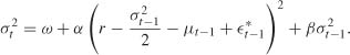
Financial Applications
In this chapter we discuss several financial applications of GARCH models. In connecting these models with those frequently used in mathematical finance, one is faced with the problem that the latter are generally written in continuous time. We start by studying the relation between GARCH and continuous-time processes. We present sufficient conditions for a sequence of stochastic difference equations to converge in distribution to a stochastic differential equation as the length of the discrete time intervals between observations goes to zero. We then apply these results to GARCH(1, 1)-type models. The second part of this chapter is devoted to the pricing of derivatives. We introduce the notion of the stochastic discount factor and show how it can be used in the GARCH framework. The final part of the chapter is devoted to risk measurement.
12.1 Relation between GARCH and Continuous-Time Models
Continuous-time models are central to mathematical finance. Most theoretical results on derivative pricing rely on continuous-time processes, obtained as solutions of diffusion equations. However, discrete-time models are the most widely used in applications. The literature on discrete-time models and that on continuous-time models developed independently, but it is possible to establish connections between the two approaches.
12.1.1 Some Properties of Stochastic Differential Equations
This first section reviews basic material from diffusion processes, which will be known to many readers. On some probability space (![]() ,
, ![]() , P), a d-dimensional process {Wt; 0 ≤ t < ∞} is called standard Brownian motion if W0 = 0 a.s., for s ≤ t, the increment Wt − Ws is independent of σ{Wu; u ≤ s] and is
, P), a d-dimensional process {Wt; 0 ≤ t < ∞} is called standard Brownian motion if W0 = 0 a.s., for s ≤ t, the increment Wt − Ws is independent of σ{Wu; u ≤ s] and is ![]() (0, (t − s)Id) distributed, where Id is the d × d identity matrix. Brownian motion is a Gaussian process and admits a version with continuous paths.
(0, (t − s)Id) distributed, where Id is the d × d identity matrix. Brownian motion is a Gaussian process and admits a version with continuous paths.
A stochastic differential equation (SDE) in ![]() p is an equation of the form
p is an equation of the form
where x0 ![]()
![]() p, μand σ are measurable functions, defined on
p, μand σ are measurable functions, defined on ![]() p and respectively taking values in
p and respectively taking values in ![]() p and
p and ![]() p × d, the space of p × d matrices. Here we only consider time-homogeneous SDEs, in which the functions μ and σ do not depend on t. A process (Xt)t
p × d, the space of p × d matrices. Here we only consider time-homogeneous SDEs, in which the functions μ and σ do not depend on t. A process (Xt)t![]() [0, T] is a solution of this equation, and Is called a diffusion process, if it satisfies
[0, T] is a solution of this equation, and Is called a diffusion process, if it satisfies
Existence and uniqueness of a solution require additional conditions on the functions μ and σ. The simplest conditions require Lipschitz and subllnearity properties:
where t ![]() [0, +∞[, x, y,
[0, +∞[, x, y, ![]()
![]() p, and K is a positive constant. In these Inequalities,
p, and K is a positive constant. In these Inequalities, ![]() ·
· ![]() denotes a norm on either
denotes a norm on either ![]() p or
p or ![]() p×d. These hypotheses also ensure the ‘nonexplosion’ of the solution on every time interval of the form [0, T] with T > 0 (see Karatzas and Schreve, 1988, Theorem 5.2.9). They can be considerably weakened, in particular when p = d = 1. The term μ(Xt) is called the drift of the diffusion, and the term σ(Xt) is called the volatility. They have the following interpretation:
p×d. These hypotheses also ensure the ‘nonexplosion’ of the solution on every time interval of the form [0, T] with T > 0 (see Karatzas and Schreve, 1988, Theorem 5.2.9). They can be considerably weakened, in particular when p = d = 1. The term μ(Xt) is called the drift of the diffusion, and the term σ(Xt) is called the volatility. They have the following interpretation:
These relations can be generalized using the second-order differential operator defined, In the case p = d = 1, by
Indeed, for a class of twice continuously differentiable functions f, we have
Moreover, the following property holds: if φ is a twice continuously differentiable function with compact support, then the process
is a martingale with respect to the filtration (Ft), where Ft is the σ -field generated by {Ws, s ≤ t). This result admits a reciprocal which provides a useful characterization of diffusions. Indeed, it can be shown that If, for a process (Xt), the process (Yt) just defined Is a Ft-martingale, for a class of sufficiently smooth functions φ, then (Xt) is a diffusion and solves (12.1).
Stationary Distribution
In certain cases the solution of an SDE admits a stationary distribution, but In general this distribution is not available in explicit form. Wong (1964) showed that, for model (12.1) in the univariate case (p = d = 1) with φ(·) ≥ 0, if there exists a function f that solves the equation
and belongs to the Pearson family of distributions, that is, of the form
where a < − 1 and b < 0, then (12.1) admits a stationary solution with density f.
Example 12.1 (Linear model) A linear SDE is an equation of the form
where ω, μ and σ are constants. For any initial value x0, this equation admits a strictly positive solution if ω ≥ 0, x0 ≥ 0 and (ω, x0) ≠ (0, 0) (Exercise 12.1). If f is assumed to be of the form (12.5), solving (12.4) leads to
Under the constraints
we obtain the stationary density
where ![]() denotes the gamma function. If this distribution is chosen for the initial distribution (that is, the law of X0), then the process (Xt) is stationary and its inverse follows a gamma distribution,1
denotes the gamma function. If this distribution is chosen for the initial distribution (that is, the law of X0), then the process (Xt) is stationary and its inverse follows a gamma distribution,1
12.1.2 Convergence of Markov Chains to Diffusions
Consider a Markov chain ![]() with values in
with values in ![]() d, indexed by the time unit τ > 0. We transform Z(τ) into a continuous-time process,
d, indexed by the time unit τ > 0. We transform Z(τ) into a continuous-time process, ![]() t
t![]()
![]() +, by means of the time interpolation
+, by means of the time interpolation
Under conditions given in the next theorem, the process ![]() converges in distribution to a diffusion. Denote by
converges in distribution to a diffusion. Denote by ![]() ·
· ![]() the Euclidean norm on
the Euclidean norm on ![]() d.
d.
Theorem 12.1 (Convergence of (![]() ) to a diffusion) Suppose there exist continuous applications μ and σ from
) to a diffusion) Suppose there exist continuous applications μ and σ from ![]() d to
d to ![]() d and
d and ![]() p × d respectively, such that for all r > 0 and for some δ > 0,
p × d respectively, such that for all r > 0 and for some δ > 0,
Then, if the equation
admits a solution (Zt) which is unique in distribution, and if ![]() converges in distribution to z0, then the process
converges in distribution to z0, then the process ![]() converges in distribution to (Zt).
converges in distribution to (Zt).
Remark 12.1 Condition (12.10) ensures, in particular, that by applying the Markov inequality, for all ![]() > 0,
> 0,
As a consequence, the limiting process has continuous paths.
Euler Discretization of a Diffusion
Diffusion processes do not admit an exact discretization in general. An exception is the geometric Brownian motion, defined as a solution of the real SDE
where μ and σ are constants. It can be shown that if the initial value x0 is strictly positive, then Xt ![]() (0, ∞) for any t > 0. By Itô’s lemma,2 we obtain
(0, ∞) for any t > 0. By Itô’s lemma,2 we obtain
and then, by Integration of this equation between times kτ and (k + l)τ, we get the discretized version of model (12.12),
For general diffusions, an explicit discretized model does not exist but a natural approximation, called the Euler discretization, is obtained by replacing the differential elements by increments. The Euler discretization of the SDE (12.1) is then given, for the time unit τ, by
The Euler discretization of a diffusion converges In distribution to this diffusion (Exercise 12.2).
Convergence of GARCH-M Processes to Diffusions
It is natural to assume that the return of a financial asset increases with risk. Economic agents who are risk-averse must receive compensation when they own risky assets. ARMA-GARCH type time series models do not take this requirement into account because the conditional mean and variance are modeled separately. A simple way to model the dependence between the average return and risk is to specify the conditional mean of the returns in the form
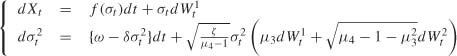
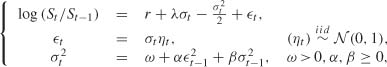
where ξ and λ are parameters. By doing so we obtain, when ![]() is specified as an ARCH, a particular case of the ARCH in mean (ARCH-M) model, introduced by Engle, Lilien and Robins (1987). The parameter λ can be interpreted as the price of risk and can thus be assumed to be positive. Other specifications of the conditional mean are obviously possible. In this section we focus on a GARCH(1, 1)-M model of the form
is specified as an ARCH, a particular case of the ARCH in mean (ARCH-M) model, introduced by Engle, Lilien and Robins (1987). The parameter λ can be interpreted as the price of risk and can thus be assumed to be positive. Other specifications of the conditional mean are obviously possible. In this section we focus on a GARCH(1, 1)-M model of the form
where ω > 0, f is a continuous function from ![]() + to
+ to ![]() , g is a continuous one-to-one map from
, g is a continuous one-to-one map from ![]() + to itself and a is a positive function. The previous interpretation implies that f is increasing, but at this point it is not necessary to make this assumption. When g(x) = x2 and a(x) = ax2 + β with α > 0, β > 0, we get the classical GARCH(1, 1) model. Asymmetric effects can be introduced, for instance by taking g(x) = x and a(x) = α+x+ − α − x− + β, with x+ = max(x, 0), x− = min(x, 0), α+ ≥ 0, α− ≥ 0, β ≥ 0.
+ to itself and a is a positive function. The previous interpretation implies that f is increasing, but at this point it is not necessary to make this assumption. When g(x) = x2 and a(x) = ax2 + β with α > 0, β > 0, we get the classical GARCH(1, 1) model. Asymmetric effects can be introduced, for instance by taking g(x) = x and a(x) = α+x+ − α − x− + β, with x+ = max(x, 0), x− = min(x, 0), α+ ≥ 0, α− ≥ 0, β ≥ 0.
Observe that the constraint for the existence of a strictly stationary and nonanticipative solution (Yt), with Yt = Xt − Xt−1, is written as
by the techniques studied in Chapter 2.
Now, in view of the Euler discretization (12.15), we introduce the sequence of models indexed by the time unit τ, defined by
for k > 0, with initial values ![]() and assuming
and assuming ![]() . The introduction of a delay k in the second equation is due to the fact that σ(k+1)τ belongs to the σ-field generated by ηkτ and its past values.
. The introduction of a delay k in the second equation is due to the fact that σ(k+1)τ belongs to the σ-field generated by ηkτ and its past values.
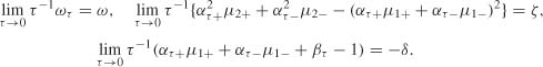
Noting that the pair Zkτ = (X(k−1)τ, g(σkτ)) defines a Markov chain, we obtain its limiting distribution by application of Theorem 12.1. We have, for z = (x, g(σ)),
This latter quantity converges if
where ω and δ are constants.
Similarly,
which converges if and only if
where ζ is a positive constant. Finally,
converges if and only if
where ρ is a constant such that ρ2 ≤ ζ.
Under these conditions we thus have
Moreover, we have
We are now in a position to state our next result.
Theorem 12.2 (Convergence of (![]() ,
, ![]() )) to a diffusion) Under Conditions (12.20), (12.23) and (12.25), and if, for δ > 0,
)) to a diffusion) Under Conditions (12.20), (12.23) and (12.25), and if, for δ > 0,
the limiting process when τ → 0, in the sense of Theorem 12.1, of the sequence of solutions of models (12.17) is the bivariate diffusion
where ![]() and
and ![]() are independent Brownian motions, with initial values x0 and σ0.
are independent Brownian motions, with initial values x0 and σ0.
Proof. It suffices to verify the conditions of Theorem 12.1. It is immediate from (12.18), (12.19), (12.21), (12.22), (12.24) and the hypotheses on f and g, that, in (12.8) and (12.9), the limits are uniform on every ball of ![]() 2. Moreover, for τ ≤ τ0 and δ < 2, we have
2. Moreover, for τ ≤ τ0 and δ < 2, we have
which is bounded uniformly in σ on every compact. On the other hand, introducing the L2+δ norm and using the triangle and Hölder’s inequalities,
Since the limit superior of this quantity, when τ → 0, is bounded uniformly in σ on every compact, we can conclude that condition (12.10) is satisfied.
It remains to show that the SDE (12.27) admits a unique solution. Note that g(σt) satisfies a linear SDE given by
where ![]() is the Brownian motion
is the Brownian motion ![]() . This equation admits a unique solution (Exercise 12.1)
. This equation admits a unique solution (Exercise 12.1)
The function g being one-to-one, we deduce σt and the solution (Xt), uniquely obtained as
Remark 12.2
1. It is interesting to note that the limiting diffusion involves two Brownian motions, whereas GARCH processes involve only one noise. This can be explained by the fact that, to obtain a Markov chain, it is necessary to consider the pair (X(k−1)τ, g(σkτ)). The Brownian motions involved in the equations of Xt and g(σt) are independent if and only if ρ = 0. This is, for instance, the case when the function aτ is even and the distribution of the iid process is symmetric.
2. Equation (12.28) shows that g(σt) is the solution of a linear model of the form (12.6). From the study of this model, we know that under the constraints
there exists a stationary distribution for g(σt). If the process is initialized with this distribution, then
Example 12.2 (GARCH(1, 1)) The volatility of the GARCH(1, 1) model is obtained for g(x) = x2, a(x) = αx2 + β. Suppose for simplicity that the distribution of the process ![]() does not depend on τ and admits moments of order 4(1 + δ), for δ > 0. Denote by μr the rth-order moment of this process. Conditions (12.20) and (12.23) take the form
does not depend on τ and admits moments of order 4(1 + δ), for δ > 0. Denote by μr the rth-order moment of this process. Conditions (12.20) and (12.23) take the form
A choice of parameters satisfying these constraints is, for instance,
Condition (12.25) is then automatically satisfied with
as well as (12.26). The limiting diffusion takes the form
and, if the law of ![]() is symmetric,
is symmetric,
Note that, with other choices of the rates of convergence of the parameters, we can obtain a limiting process involving only one Brownian motion but with a degenerate volatility equation, in the sense that it is an ordinary differential equation (Exercise 12.3).
Example 12.3 (TGARCH(1, 1)) For g(x) = x, a(x) = α+x+ − α−x− + β, we have the volatility of the threshold GARCH(1, 1) model. Under the assumptions of the previous example, let ![]() and
and ![]() . Conditions (12.20) and (12.23) take the form
. Conditions (12.20) and (12.23) take the form
These constraints are satisfied by taking, for instance, ![]() and
and
Condition (12.25) is then satisfied with ρ = α+μ2+ − α−μ2−, as well as condition (12.26). The limiting diffusion takes the form
In particular, if the law of ![]() is symmetric and if ατ+ = ατ−, the correlation between the Brownian motions of the two equations vanishes and we get a limiting diffusion of the form
is symmetric and if ατ+ = ατ−, the correlation between the Brownian motions of the two equations vanishes and we get a limiting diffusion of the form
By applying the Itô lemma to this equation, we obtain
which shows that, even in the symmetric case, the limiting diffusion does not coincide with that obtained in (12.30) for the classical GARCH model. When the law of ![]() is symmetric and ατ+ ≠ ατ−, the asymmetry in the discrete-time model results in a correlation between the two Brownian motions of the limiting diffusion.
is symmetric and ατ+ ≠ ατ−, the asymmetry in the discrete-time model results in a correlation between the two Brownian motions of the limiting diffusion.
Classical option pricing models rely on independent Gaussian returns processes. These assumptions are incompatible with the empirical properties of prices, as we saw, in particular, in the introductory chapter. It is thus natural to consider pricing models founded on more realistic, GARCH-type, or stochastic volatility, price dynamics.
We start by briefly recalling the terminology and basic concepts related to the Black-Scholes model. Appropriate financial references are provided at the end of this chapter.
12.2.1 Derivatives and Options
The need to hedge against several types of risk gave rise to a number of financial assets called derivatives. A derivative (derivative security or contingent claim) is a financial asset whose payoff depends on the price process of an underlying asset: action, portfolio, stock index, currency, etc. The definition of this payoff is settled in a contract.
There are two basic types of option. A call option (put option) or more simply a call (put) is a derivative giving to the holder the right, but not the obligation, to buy (sell) an agreed quantity of the underlying asset S, from the seller of the option on (or before) the expiration date T, for a specified price K, the strike price or exercise price. The seller (or ‘writer’) of a call is obliged to sell the underlying asset should the buyer so decide. The buyer pays a fee, called a, premium, for this right. The most common options, since their introduction in 1973, are the European options, which can be exercised only at the option expiry date, and the American options, which can be exercised at any time during the life of the option. For a European call option, the buyer receives, at the expiry date, the amount max(ST − K, 0) = (St − K)+ since the option will not be exercised unless it is ‘in the money’. Similarly, for a put, the payoff at time T is (K − ST)+. Asset pricing involves determining the option price at time t. In what follows, we shall only consider European options.
12.2.2 The Black-Scholes Approach
Consider a market with two assets, an underlying asset and a risk-free asset. The Black and Scholes (1973) model assumes that the price of the underlying asset is driven by a geometric Brownian motion
where μ and σ are constants and (Wt) is a standard Brownian motion. The risk-free interest rate r is assumed to be constant. By itô’s lemma, we obtain
showing that the logarithm of the price follows a generalized Brownian motion, with drift μ − σ2/2 and constant volatility. Integrating (12.32) between times t − 1 and t yields the discretized version
The assumption of constant volatility is obviously unrealistic. However, this model allows for explicit formulas for option prices, or more generally for any derivative based on the underlying asset S, with payoff g(ST) at the expiry date T. The price of this product at time t is unique under certain regularity conditions3 and is denoted by C(S, t) for simplicity. The set of conditions ensuring the uniqueness of the derivative price is referred to as the complete market hypothesis. In particular, these conditions imply the absence of arbitrage opportunities, that is, that there is no ‘free lunch’. It can be shown4 that the derivative price is
where the expectation is computed under the probability π corresponding to the equation
where (![]() ) denotes a standard Brownian motion. The probability π is called the risk-neutral probability, because under π the expected return of the underlying asset is the risk-free interest rate r. It is important to distinguish this from the historic probability, that is, the law under which the data are generated (here defined by model (12.31)). Under the risk-neutral probability, the price process is still a geometric Brownian motion, with the same volatility σ but with drift r. Note that the initial drift term, μ, does not play a role in the pricing formula (12.34). Moreover, the actualized price Xt = e−rt St satisfies
) denotes a standard Brownian motion. The probability π is called the risk-neutral probability, because under π the expected return of the underlying asset is the risk-free interest rate r. It is important to distinguish this from the historic probability, that is, the law under which the data are generated (here defined by model (12.31)). Under the risk-neutral probability, the price process is still a geometric Brownian motion, with the same volatility σ but with drift r. Note that the initial drift term, μ, does not play a role in the pricing formula (12.34). Moreover, the actualized price Xt = e−rt St satisfies ![]() . This implies that the actualized price is a martingale for the risk-neutral probability:
. This implies that the actualized price is a martingale for the risk-neutral probability: ![]() . Note that this formula is obvious in view of (12.34), by considering the underlying asset as a product with payoff ST at time T.
. Note that this formula is obvious in view of (12.34), by considering the underlying asset as a product with payoff ST at time T.
The Black-Scholes formula is an explicit version of (12.34) when the derivative is a call, that is, when g(ST) = (K − St)+, given by
where Ф is the conditional distribution function (cdf) of the ![]() (0, 1) distribution and
(0, 1) distribution and
In particular, it can be seen that if St is large compared to K, we have ![]() and the call price is approximately given by St − e−rτ K, that is, the current underlying price minus the actualized exercise price. The price of a put P(S, t) follows from the put-call parity relationship (Exercise 12.4): C(S, t) = P(S, t) + St − e−rτ K.
and the call price is approximately given by St − e−rτ K, that is, the current underlying price minus the actualized exercise price. The price of a put P(S, t) follows from the put-call parity relationship (Exercise 12.4): C(S, t) = P(S, t) + St − e−rτ K.
A simple computation (Exercise 12.5) shows that the European call option price is an increasing function of St, which is Intuitive. The derivative of C(S, t) with respect to St, called delta, is used in the construction of a riskless hedge, a portfolio obtained from the risk-free and risky assets allowing the seller of a call to cover the risk of a loss when the option is exercised. The construction of a riskless hedge is often referred to as delta hedging.
The previous approach can be extended to other price processes, in particular if (St) is solution of a SDE of the form
under regularity assumptions on μ and σ. When the geometric Brownlan motion for St Is replaced by another dynamics, the complete market property is generally lost.5
12.2.3 Historic Volatility and Implied Volatilities
Note that, from a statistical point of view, the sole unknown parameter in the Black-Scholes pricing formula (12.36) Is the volatility of the underlying asset. Assuming that the prices follow a geometric Brownian motion, application of this formula thus requires estimating σ. Any estimate of σ based on a history of prices S0, …, Sn is referred to as historic volatility. For geometric Brownian motion, the log-returns log(St/St−1) are, by (12.32), iid ![]() (μ − σ2/2, σ2) distributed variables. Several estimation methods for σ can be considered, such as the method of moments and the maximum likelihood method (Exercise 12.7). An estimator of C(S, t) Is then obtained by replacing σ by its estimate.
(μ − σ2/2, σ2) distributed variables. Several estimation methods for σ can be considered, such as the method of moments and the maximum likelihood method (Exercise 12.7). An estimator of C(S, t) Is then obtained by replacing σ by its estimate.
Another approach involves using option prices. In practice, traders usually work with the so-called implied volatilities. These are the volatilities Implied by option prices observed in the market. Consider a European call option whose price at time t is ![]() . If
. If ![]() denotes the price of the underlying asset at time t, an implied volatility
denotes the price of the underlying asset at time t, an implied volatility ![]() is defined by solving the equation
is defined by solving the equation
This equation cannot be solved analytically and numerical procedures are called for. Note that the solution is unique because the call price is an increasing function of σ (Exercise 12.8).
If the assumptions of the Black - Scholes model, that is, the geometric Brownian motion, are satisfied, implied volatilities calculated from options with different characteristics but the same underlying asset should coincide with the theoretical volatility σ. In practice, implied volatilities calculated with different strikes or expiration dates are very unstable, which Is not surprising since we know that the geometric Brownian motion is a misspecified model.
12.2.4 Option Pricing when the Underlying Process is a GARCH
In discrete time, with time unit δ, the binomial model (in which, given St, St+δ can only take two values) allows us to define a unique risk-neutral probability, under which the actualized price is
where Wt, ![]() are independent Brownian motions.
are independent Brownian motions.
a martingale. This model is used, in the Cox, Ross and Rubinstein (1979) approach, as an analog in discrete time of the geometric Brownian motion. Intuitively, the assumption of a complete market is satisfied (in the binomial model as well as in the Black-Scholes model) because the number of assets, two, coincides with the number of states of the world at each date. Apart from this simple situation, the complete market property is generally lost in discrete time. It follows that a multiplicity of probability measures may exist, under which the prices are martingales, and consequently, a multiplicity of pricing formulas such as (12.34). Roughly speaking, there is too much variability in prices between consecutive dates.
To determine options prices in incomplete markets, additional assumptions can be made on the risk premium and/or the preferences of the agents. A modern alternative relies on the concept of stochastic discount factor, which allows pricing formulas in discrete time similar to those in continuous time to be obtained.
Stochastic Discount Factor
We start by considering a general setting. Suppose that we observe a vector process Z = (Zt) and let It denote the information available at time t, that is, the σ-field generated by {Zs, s ≤ t}. We are interested in the pricing of a derivative whose payoff is g = g(ZT) at time T. Suppose that there exists, at time t < T, a price Ct(Z, g, T) for this asset. It can be shown that, under mild assumptions on the function ![]() ,6 we have the representation
,6 we have the representation
The variable Mt, T is called the stochastic discount factor (SDF) for the period [t, T]. The SDF introduced in representation (12.37) is not unique and can be parameterized. The formula applies, in particular, to the zero-coupon bond of expiry date T, defined as the asset with payoff 1 at time T. Its price at t is the conditional expectation of the SDF,
It follows that (12.37) can be written as
Forward Risk-Neutral Probability
Observe that the ratio Mt,T/B(t, T) is positive and that its mean, conditional on It, is 1. Consequently, a probability change removing this factor in formula (12.38) can be done.7 Denoting by πt, T the new probability and by Eπt, T the expectation under this probability, we obtain the pricing formula
The probability law πt, T is called forward risk-neutral probability. Note the analogy between this formula and (12.34), the latter corresponding to a particular form of B(t, T). To make this formula operational, it remains to specify the SDF.
As mentioned earlier, the SDF is not unique in incomplete markets. A natural restriction, referred to as a temporal coherence restriction, is given by
On the other hand, the one-step SDFs are constrained by
where St ![]() It is the price of an underlying asset (or a vector of assets). We have
It is the price of an underlying asset (or a vector of assets). We have
Noting that
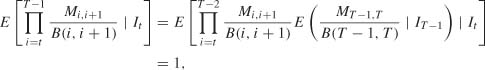
we can make a change of probability such that the SDF vanishes. Under a probability law ![]() , called risk-neutral probability, we thus have
, called risk-neutral probability, we thus have
The risk-neutral probability satisfies the temporal coherence property: ![]() is related to
is related to ![]() through the factor MT, T+1/B(T, T + 1). Without (12.40), the risk-neutral forward probability does not satisfy this property.
through the factor MT, T+1/B(T, T + 1). Without (12.40), the risk-neutral forward probability does not satisfy this property.
Pricing Formulas
One approach to deriving pricing formulas is to specify, parametrically, the dynamics of Zt and of Mt, t+1, taking (12.41) Into account.
Example 12.4 (Black-Scholes model) Consider model (12.33) with Zt = log(St/St−1) and suppose that B(t, t + 1) = e−r. A simple specification of the one-step SDF Is given by the affine model Mt +1 = exp(a + bZt+1), where a and b are constants. The constraints in (12.41) are written as
that is, in view of the ![]() (μ − σ2/2, σ2) distribution of Zt,
(μ − σ2/2, σ2) distribution of Zt,
These equations provide a unique solution (a, b). We then obtain the risk-neutral probability πt+1 = π through the characteristic function
Because the latter is the characteristic function of the ![]() (r − σ2/2, σ2) distribution, we retrieve the geometric Brownian motion model (12.35) for (St). The Black-Scholes formula is thus obtained by specifying an affine exponential SDF with constant coefficients.
(r − σ2/2, σ2) distribution, we retrieve the geometric Brownian motion model (12.35) for (St). The Black-Scholes formula is thus obtained by specifying an affine exponential SDF with constant coefficients.
Now consider a general GARCH-type model of the form
where λt and σt belong to the σ-field generated by the past of Zt, with σt > 0. Suppose that the σ -fields generated by the past of ![]() t, Zt and ηt are the same, and denote this σ -field by It−1. Suppose again that B(t, t + 1) = e−r. Consider for the SDF an affine exponential specification with random coefficients, given by
t, Zt and ηt are the same, and denote this σ -field by It−1. Suppose again that B(t, t + 1) = e−r. Consider for the SDF an affine exponential specification with random coefficients, given by
where at, bt ![]() It. The constraints (12.41) are written as
It. The constraints (12.41) are written as
that is, after simplification,
As before, these equations provide a unique solution (at, bt). The risk-neutral probability πt, t+1 is defined through the characteristic function
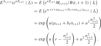
The last two equalities are obtained by taking into account the constraints on at and bt. Thus, under the probability πt, t+1, the law of the process (Zt) is given by the model
The independence of the ![]() follows from the independence between
follows from the independence between ![]() and It (because
and It (because ![]() has a fixed distribution conditional on It) and from the fact that
has a fixed distribution conditional on It) and from the fact that ![]() . The model under the risk-neutral probability is then a GARCH-type model if the variable
. The model under the risk-neutral probability is then a GARCH-type model if the variable ![]() is a measurable function of the past of
is a measurable function of the past of ![]() *t. This generally does not hold because the relation
*t. This generally does not hold because the relation
entails that the past of ![]() is included in the past of
is included in the past of ![]() t, but not the reverse.
t, but not the reverse.
If the relation (12.48) is invertible, in the sense that there exists a measurable function f such that ![]() model (12.47) is of the GARCH type, but the volatility
model (12.47) is of the GARCH type, but the volatility ![]() can take a very complicated form as a function of the
can take a very complicated form as a function of the ![]() . Specifically, if the volatility under the historic probability is that of a classical GARCH(1, 1), we have
. Specifically, if the volatility under the historic probability is that of a classical GARCH(1, 1), we have
Finally, using πt, T, the forward risk-neutral probability for the expiry date T, the price of a derivative is given by the formula
or, under the historic probability, in view of (12.40),
It is important to note that, with the affine exponential specification of the SDF, the volatilities coincide with the two probability measures. This will not be the case for other SDFs (Exercise 12.11).
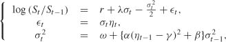
Example 12.5 (Constant coefficient SDF) We have seen that the Black-Scholes formula relies on (i) a Gaussian marginal distribution for the log-returns, and (ii) an affine exponential SDF with constant coefficients. In the framework of model (12.44), it is thus natural to look for a SDF of the same type, with at and bt independent of t. It is immediate from (12.46) that it is necessary and sufficient to take λt of the form
where μ and λ are constants. We thus obtain a model of GARCH in mean type, because the conditional mean is a function of the conditional variance. The volatility in the risk-neutral model is thus written as
If, moreover, r = μ then under the historic probability the model is expressed as
and under the risk-neutral probability,
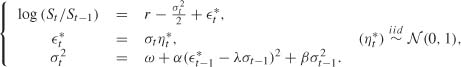
Under the latter probability, the actualized price e−rt St is a martingale (Exercise 12.9). Note that in (12.52) the coefficient λ appears in the conditional variance, but the risk has been neutralized (the conditional mean no longer depends on ![]() ). This risk-neutral probability was obtained by Duan (1995) using a different approach based on the utility of the representative agent.
). This risk-neutral probability was obtained by Duan (1995) using a different approach based on the utility of the representative agent.
Note that ![]() . Under the strict stationarity constraint
. Under the strict stationarity constraint
the variable ![]() is a function of the past of η*t and can be interpreted as the volatility of Zt under the risk-neutral probability. Under this probability, the model is not a classical GARCH(1, 1) unless λ = 0, but in this case the risk-neutral probability coincides with the historic one, which is not the case in practice.
is a function of the past of η*t and can be interpreted as the volatility of Zt under the risk-neutral probability. Under this probability, the model is not a classical GARCH(1, 1) unless λ = 0, but in this case the risk-neutral probability coincides with the historic one, which is not the case in practice.
Numerical Pricing of Option Prices
Explicit computation of the expectation involved in (12.49) is not possible, but the expectation can be evaluated by simulation. Note that, under πt, T, ST and St are linked by the formula
where ![]() . At time t, suppose that an estimate
. At time t, suppose that an estimate ![]() of the coefficients of model (12.51) is available, obtained from observations S1, …, St of the underlying asset. Simulated values
of the coefficients of model (12.51) is available, obtained from observations S1, …, St of the underlying asset. Simulated values ![]() of St, and thus simulated values
of St, and thus simulated values ![]() of ZT, for i = 1, …, N, are obtained by simulating, at step i, T − t independent realizations
of ZT, for i = 1, …, N, are obtained by simulating, at step i, T − t independent realizations ![]() of the
of the ![]() (0, 1) and by setting
(0, 1) and by setting
where the ![]() , s = t + 1, …, T, are recursively computed from
, s = t + 1, …, T, are recursively computed from
taking, for instance, as initial value ![]() , the volatility estimated from the initial GARCH model (this volatility being computed recursively, and the effect of the initialization being negligible for t large enough under stationarity assumptions). This choice can be justified by noting that for SDFs of the form (12.45), the volatilities coincide under the historic and risk-neutral probabilities. Finally, a simulation of the derivative price is obtained by taking
, the volatility estimated from the initial GARCH model (this volatility being computed recursively, and the effect of the initialization being negligible for t large enough under stationarity assumptions). This choice can be justified by noting that for SDFs of the form (12.45), the volatilities coincide under the historic and risk-neutral probabilities. Finally, a simulation of the derivative price is obtained by taking
The previous approach can obviously be extended to more general GARCH models, with larger orders and/or different volatility specifications. It can also be extended to other SDFs.
Empirical studies show that, comparing the computed prices with actual prices observed on the market, GARCH option pricing provides much better results than the classical Black-Scholes approach (see, for instance, Sabbatini and Linton, 1998; Härdle and Hafner, 2000).
To conclude this section, we observe that the formula providing the theoretical option prices can also be used to estimate the parameters of the underlying process, using observed options (see, for instance, Hsieh and Ritchken, 2005).
12.3 Value at Risk and Other Risk Measures
Risk measurement is becoming more and more important in the financial risk management of banks and other institutions involved in financial markets. The need to quantify risk typically arises when a financial institution has to determine the amount of capital to hold as a protection against unexpected losses. In fact, risk measurement is concerned with all types of risks encountered in finance. Market risk, the best-known type of risk, is the risk of change in the value of a financial position. Credit risk, also a very important type of risk, is the risk of not receiving repayments on outstanding loans, as a result borrower default. Operational risk, which has received more and more attention in recent years, is the risk of losses resulting from failed internal processes, people and systems, or external events. Liquidity risk occurs when, due to a lack of marketability, an investment cannot be bought or sold quickly enough to prevent a loss. Model risk can be defined as the risk due to the use of a misspecified model for the risk measurement.
The need for risk measurement has increased dramatically, in the last two decades, due to the introduction of new regulation procedures. In 1996 the Basel Committee on Banking Supervision (a committee established by the central bank governors in 1974) prescribed a so-called standardized model for market risk. At the same time the Committee allowed the larger financial institutions to develop their own internal model. The second Basel Accord (Basel II), initiated in 2001, considers operational risk as a new risk class and prescribes the use of finer approaches to assess the risk of credit portfolios. By using sophisticated approaches the banks may reduce the amount of regulatory capital (the capital required to support the risk), but in the event of frequent losses a larger amount may be imposed by the regulator. Parallel developments took place in the insurance sector, giving rise to the Solvency projects.
A risk measure that is used for specifying capital requirements can be thought of as the amount of capital that must be added to a position to make its risk acceptable to regulators. Value at risk (VaR) is arguably the most widely used risk measure in financial institutions. In 1993, the business bank JP Morgan publicized its estimation method, RiskMetrics, for the VaR of a portfolio. VaR is now an indispensable tool for banks, regulators and portfolio managers. Hundreds of academic and nonacademic papers on VaR may be found at http: //www.gloriamundi . org/ We start by defining VaR and discussing its properties.
Definition
VaR is concerned with the possible loss of a portfolio in a given time horizon. A natural risk measure is the maximum possible loss. However, in most models, the support of the loss distribution is unbounded so that the maximum loss is infinite. The concept of VaR replaces the maximum loss by a maximum loss which is not exceeded with a given (high) probability.
VaR should be computed using the predictive distribution of future losses, that is, the conditional distribution of future losses using the current information. However, for horizons h> 1, this conditional distribution may be hard to obtain.
To be more specific, consider a portfolio whose value at time t is a random variable denoted Vt. At horizon h, the loss is denoted
The distribution of Lt, t+h is called the loss distribution (conditional or not). This distribution is used to compute the regulatory capital which allows certain risks to be covered, but not all of them. In general, Vt is specified as a function of d unobservable risk factors.
Example 12.6 Suppose, for instance, that the portfolio is composed of d stocks. Denote by Si the price of stock i at time t and by ri, t, t+h = log Si, t+h − log Si, t the log-return. If at is the number of stocks i in the portfolio, we have
Assuming that the composition of the portfolio remains fixed between the dates t and t + h, we have
The distribution of Vt+h conditional on the available information at time t is called the profit and loss (P&L) distribution.
The determination of reserves depends on
• the portfolio,
• the available information at time t and the horizon h,8
• a level a ![]() (0, 1) characterizing the acceptable risk.9
(0, 1) characterizing the acceptable risk.9
Denote by Rt, h(α) the level of the reserves. Including these reserves, which are not subject to remuneration, the value of the portfolio at time t + h becomes Vt+h + Rt, h(α). The capital used to support risk, the VaR, also includes the current portfolio value,
and satisfies
where Pt is the probability conditional on the information available at time t.10 VaR can thus be interpreted as the capital exposed to risk in the event of bankruptcy. Equivalently,
In probabilistic terms, VaRt, h(α) is thus simply the (1 − α)-quantile of the conditional loss distribution. If, for instance, for a confidence level 99% and a horizon of 10 days, the VaR of a portfolio is €5000, this means that, if the composition of the portfolio does not change, there is a probability of 1% that the potential loss over 10 days will be larger than €5000.
Definition 12.1 The (1 − α)-quantile of the conditional loss distribution is called the VaR at the level α:
when this quantile is positive. By convention VaRt, h(α) = 0 otherwise.
In particular, it is obvious that VaRt, h(α) is a decreasing function of α.
From (12.53), computing a VaR simply reduces to determining a quantile of the conditional loss distribution. Figure 12.1 compares the VaR of three distributions, with the same variance but
Figure 12.1 VaR is the (1 − α)-quantile of the conditional loss distribution (left). The righthand graph displays the VaR as a function of α ![]() [1%, 5%] for a Gaussian distribution
[1%, 5%] for a Gaussian distribution ![]() (solid line), a Student t distribution with 3 degrees of freedom
(solid line), a Student t distribution with 3 degrees of freedom ![]() (dashed line) and a double exponential distribution ε (thin dotted line). The three laws are standardized so as to have unit variances. For α = 1% we have VaR(
(dashed line) and a double exponential distribution ε (thin dotted line). The three laws are standardized so as to have unit variances. For α = 1% we have VaR(![]() ) < VaR(
) < VaR(![]() ) < VaR(ε), whereas for α = 5% we have VaR(
) < VaR(ε), whereas for α = 5% we have VaR(![]() ) < VaR(ε) < VaR(
) < VaR(ε) < VaR(![]() ).
).
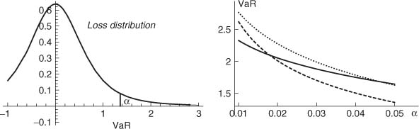
different tail thicknesses. The thickest tail, proportional to 1/x4, Is that of the Student t distribution with 3 degrees of freedom, here denoted ![]() ; the thinnest tail, proportional to
; the thinnest tail, proportional to ![]() , is that of the Gaussian
, is that of the Gaussian ![]() ; and the double exponential ε possesses a tall of Intermediate size, proportional to
; and the double exponential ε possesses a tall of Intermediate size, proportional to ![]() . For some very small level α, the VaRs are ranked in the order suggested by the thickness of the tails: VaR(
. For some very small level α, the VaRs are ranked in the order suggested by the thickness of the tails: VaR(![]() ) < VaR(ε) < VaR(
) < VaR(ε) < VaR(![]() ). However, the right-hand graph of Figure 12.1 shows that this ranking does not hold for the standard levels α = l% or α = 5%.
). However, the right-hand graph of Figure 12.1 shows that this ranking does not hold for the standard levels α = l% or α = 5%.
VaR and Conditional Moments
Let us introduce the first two moments of Lt, t+h conditional on the information available at time t:
Suppose that
where ![]() is a random variable with cumulative distribution function Fh. Denote by
is a random variable with cumulative distribution function Fh. Denote by ![]() the quantile function of the variable
the quantile function of the variable ![]() defined as the generalized Inverse of Fh:
defined as the generalized Inverse of Fh:
If Fh is continuous and strictly increasing, we simply have ![]() , where
, where ![]() is the ordinary inverse of Fh. In view of (12.53) and (12.54) it follows that
is the ordinary inverse of Fh. In view of (12.53) and (12.54) it follows that
Consequently,
VaR can thus be decomposed into an ‘expected loss’ mt, t+h, the conditional mean of the loss, and an ‘unexpected loss’ ![]() , also called economic capital.
, also called economic capital.
The apparent simplicity of formula (12.55) masks difficulties in (i) deriving the first conditional moments for a given model, and (ii) determining the law Fh, supposedly independent of t, of the standardized loss at horizon h.
Consider the price of a portfolio, defined as a combination of the prices of d assets, pt = a′ Pt, where a, Pt ![]()
![]() d. Introducing the price variations ΔPt = Pt − Pt−1, we have
d. Introducing the price variations ΔPt = Pt − Pt−1, we have
The term structure of the VaR, that is, its evolution as a function of the horizon, can be analyzed in different cases.
Example 12.7 (Independent and identically distributed price variations) If the ΔPt+i are iid ![]() (m, Σ) distributed, the law of Lt, t+h is
(m, Σ) distributed, the law of Lt, t+h is ![]() (−a′mh, a′Σah). In view of (12.55), it follows that
(−a′mh, a′Σah). In view of (12.55), it follows that
In particular, if m = 0, we have
The rale that one multiplies the VaR at horizon 1 by ![]() to obtain the VaR at horizon h is often erroneously used when the prices variations are not iid, centered and Gaussian (Exercise 12.12).
to obtain the VaR at horizon h is often erroneously used when the prices variations are not iid, centered and Gaussian (Exercise 12.12).
Example 12.8 (AR(1) price variations) Suppose now that
where A is a matrix whose eigenvalues have a modulus strictly less than 1. The process (ΔPt) is then stationary with expectation m. It can be verified (Exercise 12.13) that
where, letting At = (I − Ai)(I − A)−1,
If A = 0, (12.58) reduces to (12.56). Apart from this case, the term multiplying Ф−1(1 − α) is not proportional to ![]() .
.
Example 12.9 (ARCH(l) price variations) For simplicity let d = 1, a = 1 and
The conditional law of Lt, t+1 is ![]() (0, ω + α1ΔP2t). Therefore,
(0, ω + α1ΔP2t). Therefore,
Here VaR computation at horizons larger than 1 is problematic. Indeed, the conditional distribution of Lt, t+h is no longer Gaussian when h > 1 (Exercise 12.14).
It is often more convenient to work with the log-returns rt = Δ1 log pt,, assumed to be stationary, than with the price variations. Letting qt(h, α) be the α-quantile of the conditional distribution of the future returns rt+1 + … + rt+h, we obtain (Exercise 12.15)
VaR is often criticized for not satisfying, for any distribution of the price variations, the ‘subadditivity’ property. Subadditivity means that the VaR for two portfolios after they have been merged should be no greater than the sum of their VaRs before they were merged. However, this property does not hold: if L1 and L2 are two loss variables, we do not necessarily have, in obvious notation,
Example 12.10 (Pareto distribution) Let L1 and L2 be two independent variables, Pareto distributed, with density f(x) = (2 + x)−2 ![]() x > −1. The cdf of this distribution is F(x) = (1 − (2 + x)−1)
x > −1. The cdf of this distribution is F(x) = (1 − (2 + x)−1) ![]() x > − 1, whence the VaR at level α is Var(α) = α−1 − 2. It can be verified, for instance using Mathematica, that
x > − 1, whence the VaR at level α is Var(α) = α−1 − 2. It can be verified, for instance using Mathematica, that
Thus
It follows that ![]() . If, for instance, α = 0.01, we find
. If, for instance, α = 0.01, we find ![]() and, numerically,
and, numerically, ![]() .
.
This lack of subadditivity can be interpreted as a nonconvexity with respect to the composition of the portfolio. It means that the risk of a portfolio, when measured by the VaR, may be larger than the sum of the risks of each of its components (even when these components are independent, except in the Gaussian case). Risk management with VaR thus does not encourage diversification.
Even if VaR is the most widely used risk measure, the choice of an adequate risk measure is an open issue. As already seen, the convexity property, with respect to the portfolio composition, is not satisfied for VaR with some distributions of the loss variable. In what follows, we present several alternatives to VaR, together with a conceptualization of the ‘expected’ properties of risks measures.
Volatility and Moments
In the Markowitz (1952) portfolio theory, the variance is used as a risk measure. It might then seem natural, in a dynamic framework, to use the volatility as a risk measure. However, volatility does not take into account the signs of the differences from the conditional mean. More importantly, this measure does not satisfy some ‘coherency’ properties, as will be seen later (translation invariance, subadditivity).
Expected Shortfall
The expected shortfall (ES), or anticipated loss, is the standard risk measure used in insurance since Solvency II. This risk measure is closely related to VaR, but avoids certain of its conceptual difficulties (in particular, subadditivity). It is more sensitive then VaR to the shape of the conditional loss distribution in the tail of the distribution. In contrast to VaR, it is informative about the expected loss when a big loss occurs.
Let Lt, t+h be such that E![]() < ∞. In this section, the conditional distribution of Lt, t+h is assumed to have a continuous and strictly Increasing cdf. The ES at level α, also referred to as Tailvar, is defined as the conditional expectation of the loss given that the loss exceeds the VaR:
< ∞. In this section, the conditional distribution of Lt, t+h is assumed to have a continuous and strictly Increasing cdf. The ES at level α, also referred to as Tailvar, is defined as the conditional expectation of the loss given that the loss exceeds the VaR:
We have
Now Pt[Lt, t+h > VaRt, h(α)] = 1 − Pt[Lt, t+h ≤ VaRt, h(α)] = 1 − (1 − α) = α, where the last but one equality follows from the continuity of the cdf at VaRt, h (α). Thus
The following characterization also holds (Exercise 12.16):
ES thus can be Interpreted, for a given level α, as the mean of the VaR over all levels u ≤ α. Obviously, ESt, h(α) ≥ VaRt, h(α).
Note that the integral representation makes ESt, h (α) a continuous function of α, whatever the distribution (continuous or not) of the loss variable. VaR does not satisfy this property (for loss variables which have a zero mass over certain intervals).
Example 12.11 (The Gaussian case) If the conditional loss distribution is ![]() then, by (12.55),
then, by (12.55), ![]() , where
, where ![]() is the
is the ![]() (0, 1) cdf. Using (12.62) and introducing L*, a variable of law
(0, 1) cdf. Using (12.62) and introducing L*, a variable of law ![]() (0, 1), we have
(0, 1), we have
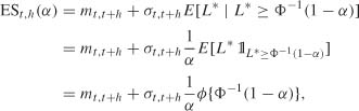
where φ Is the density of the standard Gaussian. For instance, if α = 0.05, the conditional standard deviation is multiplied by 1.65 in the VaR formula, and by 2.06 In the ES formula.
More generally, we have under assumption (12.54), in view of (12.64) and (12.55),
Distortion Risk Measures
Continue to assume that the cdf F of the loss distribution is continuous and strictly increasing. For notational simplicity, we omit the indices t and h. From (12.64), the ES is written as
where the term ![]() can be interpreted as the density of the uniform distribution over [0, α]. More generally, a distortion risk measure (DRM) is defined as a number
can be interpreted as the density of the uniform distribution over [0, α]. More generally, a distortion risk measure (DRM) is defined as a number
where G is a cdf on [0, 1], called distortion function, and F is the loss distribution. The introduction of a probability distribution on the confidence levels is often interpreted in terms of optimism or pessimism. If G admits a density g which is increasing on [0, 1], that is, if G is convex, the weight of the quantile F−1(l − u) increases with u: large risks receive small weights with this choice of G. Conversely, if G decreases, those large risks receive the bigger weights.
VaR at level α is a DRM, obtained by taking for G the Dirac mass at α. As we have seen, the ES corresponds to the constant density g on [0, α]: it is simply an average over all levels below α.
A family of DRMs is obtained by parameterizing the distortion measure as
where the parameter p reflects the confidence level, that is, the degree of optimism in the face of risk.
Example 12.12 (Exponential DRM) Let
where p ![]() ]0, +∞[. We have
]0, +∞[. We have
The density function g is decreasing whatever the value of p, which corresponds to an excessive weighting of the larger risks.
Coherent Risk Measures
In response to criticisms of VaR, several notions of coherent risk measures have been introduced. One of the proposed definitions is the following.
Definition 12.2 Let ![]() denote a set of real random loss variables defined on a measurable space (
denote a set of real random loss variables defined on a measurable space (![]() ,
, ![]() ). Suppose that
). Suppose that ![]() contains all the variables that are almost surely constant and is closed under addition and multiplication by scalars. An application ρ :
contains all the variables that are almost surely constant and is closed under addition and multiplication by scalars. An application ρ : ![]()
![]()
![]() is called a coherent risk measure if it has the following properties:
is called a coherent risk measure if it has the following properties:
1. Monotonicity: ![]() L1, L2
L1, L2 ![]()
![]() , L1 ≤ L2
, L1 ≤ L2 ![]() ρ(L1) ≤ ρ(L2).
ρ(L1) ≤ ρ(L2).
2. Subadditivity: ![]() L1, L2
L1, L2 ![]()
![]() , L1 + L2
, L1 + L2 ![]()
![]()
![]() ρ(L1 + L2) ≤ ρ(L1) + ρ(L2).
ρ(L1 + L2) ≤ ρ(L1) + ρ(L2).
3. Positive homogeneity: ![]() L
L ![]()
![]() ,
, ![]() λ ≥ 0, ρ(λL) = λρ(L).
λ ≥ 0, ρ(λL) = λρ(L).
4. Translation invariance: ![]() L
L ![]()
![]() ,
, ![]() c
c ![]()
![]() , ρ(L + c) = ρ(L) + c.
, ρ(L + c) = ρ(L) + c.
This definition has the following immediate consequences:
1. ρ(0) = 0, using the homogeneity property with L = 0. More generally, ρ(c) = c for all constants c (if a loss of amount c is certain, a cash amount c should be added to the portfolio).
2. If L ≥ 0, then ρ(L) ≥ 0. If a loss is certain, an amount of capital must be added to the position.
3. ρ(L − ρ(L)) = 0, that is, the deterministic amount ρ(L) cancels the risk of L.
These requirements are not satisfied for most risk measures used in finance. The variance, or more generally any risk measure based on the centered moments of the loss distribution, does not satisfy the monotonicity property, for instance. The expectation can be seen as a coherent, but uninteresting, risk measure. VaR satisfies all conditions except subadditivity: we have seen that this property holds for (dependent or independent) Gaussian variables, but not for general variables. ES is a coherent risk measure in the sense of Definition 12.2 (Exercise 12.17). It can be shown (see Wang and Dhaene, 1998) that DRMs with G concave satisfy the subadditivity requirement.
Unconditional VaR
The simplest estimation method is based on the K last returns at horizon h, that is, rt+h−i(h) = log(pt+h−i/pt−i), for i = h…, h + K − 1. These K returns are viewed as scenarios for future returns. The nonparametric historical VaR is simply obtained by replacing qt(h, α) in (12.60) by the empirical α-quantile of the last K returns. Typical values are K = 250 and α = 1% , which means that the third worst return is used as the empirical quantile. A parametric version is obtained by fitting a particular distribution to the returns, for example a Gaussian ![]() (μ, σ2) which amounts to replacing qt(h, α) by
(μ, σ2) which amounts to replacing qt(h, α) by ![]() +
+ ![]() Φ−1(α), where
Φ−1(α), where ![]() and
and ![]() are the estimated mean and standard deviation. Apart from the (somewhat unrealistic) case where the returns are iid, these methods have little theoretical justification.
are the estimated mean and standard deviation. Apart from the (somewhat unrealistic) case where the returns are iid, these methods have little theoretical justification.
RiskMetrics Model
A popular estimation method for the conditional VaR relies on the RiskMetrics model. This model is defined by the equations
where λ ![]() ]0, 1[ is a smoothing parameter, for which, according to RiskMetrics (Longerstaey, 1996), a reasonable choice is λ = 0.94 for daily series. Thus,
]0, 1[ is a smoothing parameter, for which, according to RiskMetrics (Longerstaey, 1996), a reasonable choice is λ = 0.94 for daily series. Thus, ![]() is simply the prediction of
is simply the prediction of ![]() obtained by simple exponential smoothing. This model can also be viewed as an IGARCH(1, 1) without intercept. It is worth noting that no nondegenerate solution (rt)t
obtained by simple exponential smoothing. This model can also be viewed as an IGARCH(1, 1) without intercept. It is worth noting that no nondegenerate solution (rt)t![]()
![]() to (12.66) exists (Exercise 12.18). Thus, (12.66) is not a realistic data generating process for any usual financial series. This model can, however, be used as a simple tool for VaR computation. From (12.60), we get
to (12.66) exists (Exercise 12.18). Thus, (12.66) is not a realistic data generating process for any usual financial series. This model can, however, be used as a simple tool for VaR computation. From (12.60), we get
Let ![]() t denote the information generated by
t denote the information generated by ![]() t,
t, ![]() t−1, …,
t−1, …, ![]() 1. Choosing an arbitrary initial value to
1. Choosing an arbitrary initial value to ![]() , we obtain
, we obtain ![]()
![]()
![]() t and
t and
for i ≥ 2. It follows that Var![]() . Note however that the conditional distribution of rt+1 + … + rt+h is not exactly
. Note however that the conditional distribution of rt+1 + … + rt+h is not exactly ![]() (0,
(0, ![]() ) (Exercise 12.19). Many practitioners, however, systematically use the erroneous formula
) (Exercise 12.19). Many practitioners, however, systematically use the erroneous formula
Of course, one can use more sophisticated GARCH-type models, rather than the degenerate version of RiskMetries. To estimate VaRt(l, α) it suffices to use (12.60) and to estimate qt(l, α) by ![]() , where
, where ![]() is the conditional variance estimated by a GARCH-type model (for instance, an EGARCH or TGARCH to account for the leverage effect; see Chapter 10), and
is the conditional variance estimated by a GARCH-type model (for instance, an EGARCH or TGARCH to account for the leverage effect; see Chapter 10), and ![]() is an estimate of the distribution of the normalized residuals. It is, however, important to note that, even for a simple Gaussian GARCH(1, 1), there is no explicit available formula for computing qt(h, α) when h > 1. Apart from the case h = 1, simulations are required to evaluate this quantile (but, as can be seen from Exercise 12.19, this should also be the case with the RiskMetrics method). The following procedure may then be suggested:
is an estimate of the distribution of the normalized residuals. It is, however, important to note that, even for a simple Gaussian GARCH(1, 1), there is no explicit available formula for computing qt(h, α) when h > 1. Apart from the case h = 1, simulations are required to evaluate this quantile (but, as can be seen from Exercise 12.19, this should also be the case with the RiskMetrics method). The following procedure may then be suggested:
(a) Fit a model, for instance a GARCH(1, 1), on the observed returns rt = ![]() t, t = 1, …, n, and deduce the estimated volatility
t, t = 1, …, n, and deduce the estimated volatility ![]() for t = 1, …, n + 1.
for t = 1, …, n + 1.
(b) Simulate a large number N of scenarios for ![]() n+1, …,
n+1, …, ![]() n+h by iterating, independently for i = 1, …, N, the following three steps:
n+h by iterating, independently for i = 1, …, N, the following three steps:
(bl) simulate the values ![]() iid with the distribution
iid with the distribution ![]() ;
;
(b2) set ![]() =
= ![]() and
and ![]() =
= ![]() ;
;
(b3) for k = 2, …,h, set ![]() and =
and = ![]() =
= ![]()
(c) Determine the empirical quantile of simulations ![]() , i = 1,…, N.
, i = 1,…, N.
The distribution ![]() can be obtained parametrically or nonparametrically. A simple nonparametric method involves taking for
can be obtained parametrically or nonparametrically. A simple nonparametric method involves taking for ![]() the empirical distribution of the standardized residuals
the empirical distribution of the standardized residuals ![]() , which amounts to taking, in step (bl), a bootstrap sample of the standardized residuals.
, which amounts to taking, in step (bl), a bootstrap sample of the standardized residuals.
Assessment of the Estimated YaR (Backtesting)
The Basel accords allow financial institutions to develop their own internal procedures to evaluate their techniques for risk measurement. The term ‘backtesting’ refers to procedures comparing, on a test (out-of-sample) period, the observed violations of the VaR (or any other risk measure), the latter being computed from a model estimated on an earlier period (in-sample).
To fix ideas, define the variables corresponding to the violations of VaR (‘hit variables’)
Ideally, we should have
that is, a correct proportion of effective losses which violate the estimated VaRs, with a minimal average cost.
Numerical Illustration
Consider a portfolio constituted solely by the CAC 40 index, over the period from March 1, 1990 to April 23, 2007. We use the first 2202 daily returns, corresponding to the period from March 2, 1990 to December 30, 1998, to estimate the volatility using different methods. To fix ideas, suppose that on December 30, 1998 the value of the portfolio was, In French Francs, the equivalent of €;l million. For the second period, from January 4, 1999 to April 23, 2007 (2120 values), we estimated VaR at horizon h = 1 and level α = 1% using four methods.
The first method (historical) is based on the empirical quantiles of the last 250 returns. The second method is RiskMetrics. The initial value for ![]() was chosen equal to the average of the squared last 250 returns of the period from March 2, 1990 to December 30, 1998, and we took λ = 0.94. The third method (GARCH-
was chosen equal to the average of the squared last 250 returns of the period from March 2, 1990 to December 30, 1998, and we took λ = 0.94. The third method (GARCH-![]() ) relies on a GARCH(1, 1) model with Gaussian
) relies on a GARCH(1, 1) model with Gaussian ![]() (0, 1) innovations. With this method we set
(0, 1) innovations. With this method we set ![]() (0.01) = −2.32635, the 1% quantile of the
(0.01) = −2.32635, the 1% quantile of the ![]() (0, 1) distribution. The last method (GARCH-NP) estimates volatility using a GARCH(1, 1) model, and approximates
(0, 1) distribution. The last method (GARCH-NP) estimates volatility using a GARCH(1, 1) model, and approximates ![]() (0.01) by the empirical 1% quantile of the standardized residuals. For the last two methods, we estimated a GARCH(1, 1) on the first period, and kept this GARCH model for all VaR estimations of the second period. The estimated VaR and the effective losses were compared for the 2120 data of the second period.
(0.01) by the empirical 1% quantile of the standardized residuals. For the last two methods, we estimated a GARCH(1, 1) on the first period, and kept this GARCH model for all VaR estimations of the second period. The estimated VaR and the effective losses were compared for the 2120 data of the second period.
Table 12.1 and Figure 12.2 do not allow us to draw definitive conclusions, but the historical method appears to be outperformed by the NP-GARCH method. On this example, the only method
Table 12.1 Comparison of the four VaR estimation methods for the CAC 40. On the 2120 values, the VaR at the 1% level should only be violated 2120 × 1% = 21.2 times on average.
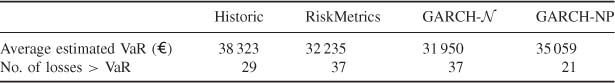
Figure 12.2 Effective losses of the CAC 40 (solid lines) and estimated VaRs (dotted lines) in thousands of euros for the historical method (top left), RiskMetrics (top right), GARCH-![]() (bottom left) and GARCH-NP (bottom right).
(bottom left) and GARCH-NP (bottom right).
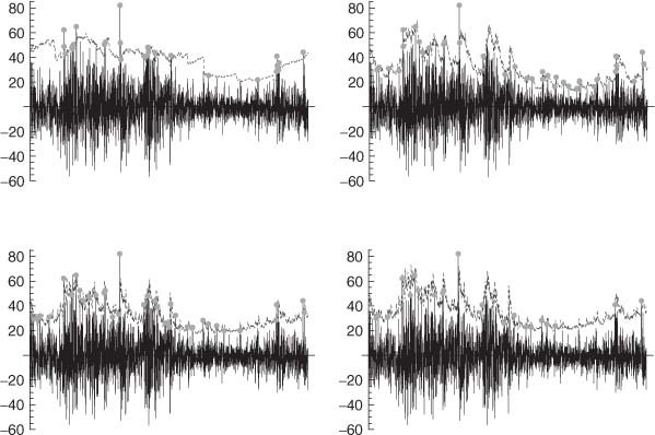
which adequately controls the level 1% is the NP-GARCH, which is not surprising since the empirical distribution of the standardized residuals is very far from Gaussian.
A detailed presentation of the financial concepts introduced in this chapter is provided in the books by Gourieroux and Jasiak (2001) and Franke, Härdle and Hafner (2004). A classical reference on the stochastic calculus is the book by Karatzas and Shreve (1988).
The relation between continuous-time processes and GARCH processes was established by Nelson (1990b) (see also Nelson, 1992; Nelson and Foster, 1994, 1995). The results obtained by Nelson rely on concepts presented in the monograph by Stroock and Varadhan (1979). A synthesis of these results is presented in File (1994). An application of these techniques to the TARCH model with contemporaneous asymmetry is developed in El Babsiri and Zakoïan (1990).
When applied to high-frequency (intraday) data, diffusion processes obtained as GARCH limits when the time unit tends to zero are often found inadequate, in particular because they do not allow for daily periodicity. There is a vast literature on the so-called realized volatility, which is a daily measure of daily return variability. See Barndorff-Nielsen and Shephard (2002) and Andersen et al. (2003) for econometric approaches to realized volatility. In the latter paper, it is argued that ‘standard volatility models used for forecasting at the daily level cannot readily accommodate the information in intraday data, and models specified directly for the intraday data generally fail to capture the longer interdaily volatility movements sufficiently well’. Another point of view is defended in the recent thesis by Visser (2009) in which it is shown that intraday price movements can be incorporated into daily GARCH models.
Concerning the pricing of derivatives, we have purposely limited our presentation to the elementary definitions. Specialized monographs on this topic are those of Dana and Jeanblanc-Picquá (1994) and Duffle (1994). Many continuous-time models have been proposed to extend the Black and Scholes (1973) formula to the case of a nonconstant volatility. The Hull and White (1987) approach introduces a stochastic differential equation for the volatility but is not compatible with the assumption of a complete market. To overcome this difficulty, Hobson and Rogers (1998) developed a stochastic volatility model in which no additional Brownian motion is introduced. A discrete-time version of this model was proposed and studied by Jeantheau (2004).
The characterization of the risk-neutral measure in the GARCH case is due to Duan (1995). Numerical methods for computing option prices were developed by Engle and Mustafa (1992) and Heston and Nandi (2000), among many others. Problems of option hedging with pricing models based on GARCH or stochastic volatility are discussed in Garcia, Ghysels and Renault (1998). The empirical performance of pricing models in the GARCH framework is studied by Härdle and Hafner (2000), Christoffersen and Jacobs (2004) and the references therein. Valuation of American options in the GARCH framework is studied in Duan and Simonato (2001) and Stentoft (2005). The use of the realized volatility, based on high-frequency data is considered in Stentoft (2008). Statistical properties of the realized volatility in stochastic volatility models are studied by Barndorff-Nielsen and Shephard (2002).
Introduced by Engle, Lilien and Robins (1987), ARCH-M models are characterized by a linear relationship between the conditional mean and variance of the returns. These models were used to test the validity of the intertemporal capital asset pricing model of Merton (1973) which postulates such a relationship (see, for instance, Lanne and Saikkonen, 2006). To our knowledge, the asymptotic properties of the QMLE have not been established for ARCH-M models.
The concept of the stochastic discount factor was developed by Hansen and Richard (1987) and, more recently, by Cochrane (2001). Our presentation follows that of Gourieroux and Tiomo (2007). This method is used in Bertholon, Monfort and Pegoraro (2008).
The concept of coherent risk measures (Definition 12.2) was introduced by Artzner et al. (1999), initially on a finite probability space, and extended by Delbaen (2002). In the latter article it Is shown that, for the existence of coherent risk measures, the set ![]() cannot be too large, for instance the set of all absolutely continuous random variables. Alternative axioms were introduced by Wang, Young and Panjer (1997), initially for risk analysis in insurance. Dynamic VaR models were proposed by Koenker and Xiao (2006) (quantile autoregressive models), Engle and Manganelli (2004) (conditional autoregressive VaR), Gouriéroux and Jasiak (2008) (dynamic additive quantile). The issue of assessing risk measures was considered by Christoffersen (1998), Christoffersen and Pelletier (2004), Engle and Manganelli (2004) and Hurlin and Tokpavi (2006), among others. The article by Escanciano and Olmo (2010) considers the impact of parameter estimation In risk measure assessment. Evaluation of VaR at horizons longer than 1, under GARCH dynamics, is discussed by Ardia (2008).
cannot be too large, for instance the set of all absolutely continuous random variables. Alternative axioms were introduced by Wang, Young and Panjer (1997), initially for risk analysis in insurance. Dynamic VaR models were proposed by Koenker and Xiao (2006) (quantile autoregressive models), Engle and Manganelli (2004) (conditional autoregressive VaR), Gouriéroux and Jasiak (2008) (dynamic additive quantile). The issue of assessing risk measures was considered by Christoffersen (1998), Christoffersen and Pelletier (2004), Engle and Manganelli (2004) and Hurlin and Tokpavi (2006), among others. The article by Escanciano and Olmo (2010) considers the impact of parameter estimation In risk measure assessment. Evaluation of VaR at horizons longer than 1, under GARCH dynamics, is discussed by Ardia (2008).
12.1 (Linear SDE)
Consider the linear SDE (12.6). Letting ![]() denote the solution obtained for ω = 0, what is the equation satisfied by Yt = Xt/
denote the solution obtained for ω = 0, what is the equation satisfied by Yt = Xt/![]() ?
?
Hint: the following result, which is a consequence of the multidimensional Itô formula, can be used. If X = (![]() ,
, ![]() ) Is a two-dimensional process such that, for a real Brownian motion (Wt),
) Is a two-dimensional process such that, for a real Brownian motion (Wt),
under standard assumptions, then
Deduce the solution of (12.6) and verify that if ω ≥ 0, x0 ≥ 0 and (ω, x0) ≠ (0, 0), then this solution will remain strictly positive.
12.2 (Convergence of the Eider discretization)
Show that the Euler discretization (12.15), with μ and σ continuous, converges in distribution to the solution of the SDE (12.1), assuming that this equation admits a unique (in distribution) solution.
12.3 (Another limiting process for the GARCH (1, 1) (Corradi, 2000))
Instead of the rates of convergence (12.30) for the parameters of a GARCH(1, 1), consider
Give an example of the sequence (ωτ, ατ, βτ) compatible with these conditions. Determine the limiting process of (![]() ,
, ![]() when τ → 0. Show that, in this model, the volatility
when τ → 0. Show that, in this model, the volatility ![]() has a nonstochastic limit when t → ∞.
has a nonstochastic limit when t → ∞.
12.4 (Put-call parity)
Using the martingale property for the actualized price under the risk-neutral probability, deduce the European put option price from the European call option price.
12.5 (Delta of a European call)
Compute the derivative with respect to St of the European call option price and check that it is positive.
12.6 (Volatility of an option price)
Show that the European call option price Ct = C(S, t) Is solution of an SDE of the form
with σt > σ.
12.7 (Estimation of the drift and volatility)
Compute the maximum likelihood estimators of μ and σ2 based on observations S1, …, Sn of the geometric Brownian motion.
12.8 (Vega of a European call)
A measure of the sensitivity of an option to the volatility of the underlying asset is the so-called vega coefficient defined by ∂Ct/∂σ. Compute this coefficient for a European call and verify that it is positive. Is this intuitive?
12.9 (Martingale property under the risk-neutral probability)
Verify that under the measure π defined in (12.52), the actualized price e−rt St is a martingale.
12.10 (Risk-neutral probability for a nonlinear GARCH model)
Duan (1995) considered the model
where ω > 0, α, β ≥ 0 and ![]() (0, 1). Establish the strict and second-order statlonarity conditions for the process (
(0, 1). Establish the strict and second-order statlonarity conditions for the process (![]() t). Determine the risk-neutral probability using stochastic discount factors, chosen to be affine exponential with time-dependent coefficients.
t). Determine the risk-neutral probability using stochastic discount factors, chosen to be affine exponential with time-dependent coefficients.
12.11 (A nonaffine exponential SDF)
Consider an SDF of the form
Show that, by an appropriate choice of the coefficients at, bt and ct, with ct ≠ 0, a risk-neutral probability can be obtained for model (12.51). Derive the risk-neutral version of the model and verify that the volatility differs from that of the initial model.
12.12 (An erroneous computation of the VaR at horizon h.)
The aim of this exercise is to show that (12.57) may be wrong if the price variations are iid but non-Gaussian. Suppose that (a′ΔPt) is iid, with a double exponential density with parameter λ, given by f (x) = 0.5λ exp{−λ|x|}. Calculate VaRt, 1(α). What Is the density of Lt, t+2? Deduce the equation for VaR at horizon 2. Show, for instance for λ = 0.1, that VaR is overevaluated if (12.57) is applied with α = 0.01, but is underevaluated with α = 0.05.
12.13 (VaR for AR(l) prices variations.)
Check that formula (12.58) is satisfied.
12.14 (VaR for ARCH(1) prices variations.)
Suppose that the price variations follow an ARCH(l) model (12.59). Show that the distribution of ΔPt+2 conditional on the information at time t is not Gaussian if α1 > 0. Deduce that VaR at horizon 2 Is not easily computable.
12.15 (VaR and conditional quantile)
Derive formula (12.60), giving the relationship between VaR and the returns conditional quantile.
12.16 (Integral formula for the ES)
Using the fact that Lt, t+h and F−1(U) have the same distribution, where U denotes a variable uniformly distributed on [0, 1] and F the cdf of Lt, t+h, derive formula (12.64).
12.17 (Coherence of the ES)
Prove that the ES is a coherent risk measure.
Hint for proving subadditivity: For Lt such that ![]() , i = 1, 2, 3, denote the value at risk at level α by VaRi;(α) and the expected shortfall by
, i = 1, 2, 3, denote the value at risk at level α by VaRi;(α) and the expected shortfall by ![]() . For L3 = L1 + L2, compute α{ES1 (α) + ES2(α) − ES3(α)} using expectations and observe that
. For L3 = L1 + L2, compute α{ES1 (α) + ES2(α) − ES3(α)} using expectations and observe that
12.18 (RiskMetrics is a prediction method, not really a model)
For any initial value ![]() let (
let (![]() t)t ≥ 1 be a sequence of random variables satisfying the Risk-Metrics model (12.66) for any t ≥ 1. Show that
t)t ≥ 1 be a sequence of random variables satisfying the Risk-Metrics model (12.66) for any t ≥ 1. Show that ![]() t → 0 almost surely as t → ∞.
t → 0 almost surely as t → ∞.
12.19 (At horizon h >1 the conditional distribution of the future returns is not Gaussian with RiskMetrics)
Prove that in the RiskMetrics model, the conditional distribution of the returns at horizon 2, rt+1 + rt+2, is not Gaussian. Conclude that formula (12.67) is incorrect.
1 The Г(a, b) density, for a, b > 0, is defined on ![]() + by
+ by
![]()
2 For Yt = f(t, Xt) where f :(t, x) ![]() [0, T] ×
[0, T] × ![]()
![]() f(t, x)
f(t, x) ![]()
![]() is continuous, continuously differentiable with respect to the first component and twice continuously differentiable with respect to the second component, if (Xt) satisfies dXt = μtdt + σtdWt where μt and σt are adapted processes such that a.s.
is continuous, continuously differentiable with respect to the first component and twice continuously differentiable with respect to the second component, if (Xt) satisfies dXt = μtdt + σtdWt where μt and σt are adapted processes such that a.s. ![]() and
and ![]() , we have
, we have ![]()
3 These conditions are the absence of transaction costs, the possibility of constructing a portfolio with any allocations (sign and size) of the two assets, the possibility of continuously adjusting the composition of the portfolio and the existence of a price for the derivative depending only on the present and past values of St.
4 The three classical methods for proving this formula are the method based on the binomial model (Cox, Ross and Rubinstein, 1979), the method based on the resolution of equations with partial derivatives and the method based on the martingale theory.
5 This is the case for the stochastic volatility model of Hull and White (1987), defined by
![]()
6 In particular, linearity and positivity (see Hansen and Richard, 1987; Gouriéroux and Tiomo, 2007).
7 If X is a random variable with distribution Px and G is a function with real positive values such that E{G(X)} = 1, we have, interpreting G as the density of some measure ![]() with respect to Px,
with respect to Px, ![]()
8 For market risk management, h is typically 1 or 10 days. For the regulator (concerned with credit or operational risk) h is 1 year.
9 1 − α is often referred to as the confidence level. Typical values of α are 5% or 3%.
10 In the ‘standard’ approach, the conditional distribution is replaced by the unconditional.