
13
Optimizing Practical Planning for Game AI
Éric Jacopin
13.1 Introduction
Planning generates sequences of actions called plans. Practical planning for game artificial intelligence (AI) refers to a planning procedure that fits in the AI budget of a game and supports playability so that nonplayer characters (NPCs) execute actions from the plans generated by this planning procedure.
Jeff Orkin developed Goal-Oriented Action Planning (GOAP) [Orkin 04] as the first ever implementation of practical planning for the game [F.E.A.R. 05]. GOAP implements practical planning with (1) actions as C++ classes, (2) plans as paths in a space of states, and (3) search as path planning in a space of states, applying actions backwardly from the goal state to the initial state; moreover, GOAP introduced action costs as a search heuristic. Many games used GOAP since 2005, and it is still used today, for example, [Deus Ex 3 DC 13] and [Tomb Raider 13], sometimes with forward search, which seems easier to debug, as the most noticeable change.
In this chapter, we present how to optimize a GOAP-like planning procedure with actions as text files [Cheng 05] and forward breadth-first search (refer to Section A.2 of [Ghallab 04]) so that it becomes practical to implement planning. Actions as text files allow nonprogrammers to provide actions iteratively without recompiling the game project: nonprogrammers can modify and update the action files during game development and debugging. That is, planning ideas can be developed and validated offline. Moreover, if needed, C++ can always be generated from the text files and included in the code of your planner at any time during development.
Forward breadth-first search is one of the simplest search algorithms since it is easy to understand, extra data structures are not required prior to search, and short plans are found faster and with less memory than other appealing plan-graph-based planning procedures [Ghallab 04, Chapter 6]. Last, it is also a complete search procedure that returns the shortest plans; NPCs won’t get redundant or useless actions to execute.
This chapter will first present the necessary steps before going into any optimization campaign, with examples specific to practical planning. Next, we will describe what can be optimized in practical planning, focusing on practical planning data structures that lead to both runtime and memory footprint improvements.
13.1.1 Required Background
The reader is expected to have a basic knowledge of GOAP [Orkin 04], predicate-based state and action representation [Cheng 05, Ghallab 04, Chapter 2], and basic search techniques (e.g., breadth-first search) as applied to planning [Ghallab 04, Chapter 4].
13.2 How Can You Optimize?
There are two main features to optimize in practical planning: time and memory. Ideally, we want to minimize both, but ultimately which one to focus on depends on the criteria of your game. Additionally, most algorithms can trade memory for time or vice versa.
13.2.1 Measure It!
Your first step is to get some code in order to measure both time and memory usage. The objective here is to instrument your practical planning code easily and quickly to show improvements in runtime and memory usage with respect to the allowed budgets.
Runtime measurement is not as easy as it sounds. Often, you’ll get varied results even when the timings were performed under the same testing conditions. So an important aspect is to decide on a unit of time that has enough detail. Several timings under the same testing conditions should provide enough significant digits, with their numerical values being very close. If you’re going to improve runtime by two orders of magnitude, you need to start with at least 4 significant digits. C++11 provides the flexible std::chrono library [Josuttis 13] that should fit most of your needs, but any platform-specific library providing a reliable high-resolution counter should do the job. Using microseconds is a good start.
With no (unpredictable) memory leak, memory measures are stable and must return the exact same value under the same testing conditions. The first step here is to measure memory overhead; for instance, an empty std::vector takes 16 bytes with Microsoft’s Visual C++ 2013, while an empty std::valarray takes only 8 bytes if you can use it instead (they only store numeric values; they cannot grow but they can be resized), and there’s no memory overhead for an instance of std::array, again if you can use it (they are C-style arrays: their size is fixed). The second step is to decide whether any measure is at all relevant; for instance, do you want to count distinct structures or the whole memory page that was allocated to store these structures?
Finally, you’ll have to decide between using conditional compiling to switch on and off the call to measures, assuming the linker shall not include the unnecessary measurement code when switched off, or a specific version of your practical planner that shall have to be synchronized with further updated versions of the planner.
13.2.2 Design Valuable Tests!
The second step is to design a set of planning tests.
A first set of planning tests is necessary in order to confirm the planner generates correct plans, that is, plans that are solutions to the planning problems of your game. If your planner uses a complete search procedure such as breadth-first search, the correct plans should also be the shortest ones. By running your planner against these gaming problems, your objective is to show this planner can be used in your game. Do not consider only planning problems related to your game, because these problems certainly are too small to stress the full power of a GOAP-like planner. On one hand, a GOAP-like planner generates less than one plan per second per NPC on average, and on another hand, these plans are very short, say, at most four actions. Consequently, a second set of complex planning tests is needed to show any improvement in the optimization process. Runtime for such complex tests can be up to several minutes, whereas in-game planning runtime, it is at most several milliseconds. There are two kinds of complex tests: scaling tests and competition tests.
First, scaling tests provide an increasing number of one specific game object: box, creature, location, vehicle, weapon, and so forth. Solution plans to scaling tests can be short, and plan length is expected to be the same for all of the scaling tests; the idea is to provide more objects of one kind than would ever happen in a gaming situation so that the branching factor in the search space explodes, although the solution is the same. For instance, and this is valid for a forward state space GOAP-like procedure, take an in-game planning problem such that the goal situation involves only one box; assume that this box, say box-1, has to be picked up at one location and moved to another location. Then build an initial situation with increasing number of boxes: box-2, box-3, and so on, although box-1 is still the only box that appears in the goal solution. As the planner can pick up one box, it shall try to pick up and then move each box until the goal solution, which only requires box-1, is reached.
Second, competition tests are complex problems whose objective is to swallow a lot of computing resources with the help of a high branching factor and a solution with a long sequence of actions [IPC 14]. For instance, it is now time to move several boxes to the final location. This requires that you allow for picking up and moving only one box at a time and do not impose priorities between boxes. There are consequently many solutions of the exact same length. Each of these solutions reflects the order in which the boxes reach the goal location, thus entailing a huge search space.
Of course, if any updated version of the planning code shows a performance decrease against these planning problems, then this update is not an improvement.
13.2.3 Use Profilers!
There is no way to escape the use of profilers.
With the first two steps, you are able to show your practical planner is usable for your game and that your latest code update is either an improvement or else a bad idea. But how are you going to improve more, avoid bad ideas, or discover unexpected and eventually fruitful paths? Runtime and memory profilers are here to help.
On the contrary to the quick and easy first two steps that both are matters of days, this third step is a matter of weeks and months. Either you use professional tools (e.g., Intel® VTunes™ and IBM® Rational® Purify Plus that both allow to profile source code and binaries) or else you’ll need to develop specific in-game profiling tools [Rabin 00, Lung 11]. Using professional tools requires mastering them, while making your own definitively requires development time. Either way, an investment of time will need to be made.
By reporting where the computing resources go, these tools tell you where to focus your improvement effort, and this is invaluable. If, on this improvement path, you reach a point where no part of your code seems to stand out as a candidate for improvement, then, beyond changing the profiling scheme and counters and running the tests again, it might be time to settle down and think of your planning data structures and your planning algorithms.
13.3 Practical Planning Data Structures
From a far viewpoint, anything can be optimized, from parsing the action text files to the data structure holding the solution to the planning problem. There is also the planning domain (how actions are encoded) and the planning problems (how states, either initial or goal, are encoded) using properties of your game world [Cheng 05, pp. 342–343]. For instance, you may not wish to represent the details of navigation from one location to another (e.g., navigating into a building, unlocking, and opening doors, avoiding obstacles) or the necessary actions to solve a puzzle in the planning problem; instead, encode only one action that magically reaches the goal location or magically solves the puzzle; then, delegate the execution of this action to a specific routine. Our focus here is different.
From a closer viewpoint, we learn from computational complexity that time complexity cannot be strictly less than space complexity [Garey 79, p. 170]; that is, at best, the computation time shall grow (with respect to a given parameter, e.g., the number of predicates) as the amount of memory needed for this computation, but never less. Consequently, you can design better algorithms to achieve better runtimes, but you can also design better data structures and start with shrinking memory: use as less memory as you can and use it as best as you can [Rabin 11].
First, make sure to choose the smallest structure that supports the features you need. Then, avoid multiple copies of these structures by storing information only once, and share it everywhere it is needed [Noble 01, pp. 182–190]. For instance, the action text files may contain several occurrences of the same identifier; when reading the first occurrence of this identifier, push it in an std::vector and share its position:
std::vector<Identifier> theIdentifiers;
size_t AddIdentifier(Identifier& id)
{
size_t position = theIdentifiers.size();
theIdentifiers.push_back(id);
return position;
}
Of course, the next occurrence of id in the text file must not be pushed at the back of theIdentifiers but must be retrieved in theIdentifiers in order to share its position. So you may want instead to hash identifiers in an std::unordered_map, storing an integer value at the hashed position, and increment this value each time a new identifier is added to the table:
std::unordered_map<Identifier, size_t> theIdentifiers;
size_t AddIdentifier(Identifier& id)
{
size_t position = theIdentifiers.size();
theIdentifiers[id] = position;
return position;
}
Lookup and sharing is then achieved through an iterator:
size_t shared_position;
std::unordered_map<Identifier, size_t>::iterator it;
it = theIdentifiers.find(id);
if (theIdentifiers.end() == it)
shared_position = AddIdentifier(id);
else
shared_position = it->second;
When the parsing of the action text file ends, we know exactly how many distinct identifiers are in the action text file and thus can allocate an array and move the identifiers from the hash table to their position in the array. More space can be saved as soon as we know the number of distinct identifiers: that is, use an unsigned char, instead of size_t in the aforementioned code, to share the positions when there are less than 256 identifiers for your planning problems, and so on.
Finally, consider a custom memory allocator (even for the STL [Isensee 03]) to access memory quicker than the classical memory allocation routines (e.g., malloc). Several high-performance memory allocators are available [Berger 14, Lazarov 08, Lea 12, Masmano 08] with various licensing schemes. Try them or any other one before embarking into developing your own.
Assuming that predicates can share their position to other planning data structures, the rest of this section discusses the use of the sharing pattern [Noble 01, pp. 182–190] to actions, plans, and states.
13.3.1 Actions
An action is made of two sets of predicates, in the spirit of IF/THEN rules [Wilhelm 08]: the set of preconditions predicates and the set of postcondition predicates (effects). A predicate can only occur in both sets if and only if it is negative (prefixed by not) in one set and positive in the other set. For instance, the positive predicate hold(gun) can appear as a precondition of the action Drop if the negative predicate not(hold(gun)) is one of its effects; accordingly (i.e., symmetrically), hold(gun) can be an effect of the action Take if not(hold(gun)) is one of its preconditions.
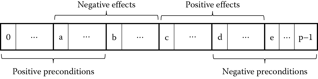
Assume an array of shared positions of predicates, ranging from 0 to (p − 1). Then the action predicates can be ordered in the array so that they occur only once:
- Let a, b, c, d, e, and p such that 0 ≤ a ≤ b ≤ c ≤ d ≤ e ≤ (p − 1).
- [0, a − 1] is the range of positive preconditions.
- [a, b − 1] is the range of positive preconditions that occur as negative effects.
- [b, c − 1] is the range of negative effects.
- [c, d − 1] is the range of positive effects.
- [d, e − 1] is the range of positive effects that occur as negative preconditions.
- [e, p − 1] is the range of negative preconditions.
Consequently, preconditions are in the range [0, b − 1] and in the range [d, p − 1], and effects are in the range [a, e − 1] as illustrated in Figure 13.1.
For instance, the positive predicate hold(gun) of the action Drop shall occur in the range [a, b − 1], whereas it shall occur in the range [d, e − 1] for the action Take (which is detailed in a following section).
Moreover, an action has parameters that are shared among its predicates; for instance, both the actions Drop and Take have an object as a parameter for the predicate hold. If we further constrain all predicate parameters to be gathered in the set of parameters of an action, then all predicate parameters only need to be integer values pointing to the positions of the parameters of their action; the type unsigned char can be used for these integer values if we limit the number of parameters to 256, which is safe.
13.3.2 Plans
A GOAP-like plan is a totally ordered set of actions. An action is uniquely represented by an action identifier, for example, Drop, and its parameters (once they all have a value), which is called the action signature, for example, Drop(gun). An action signature is a good candidate for sharing its position in an array. Consequently, a plan is an array of shared positions of action signatures.
As plans grow during the search, using an std::vector is practical, while keeping in mind the memory overhead for std::vectors. Assume the 16 bytes of Visual C++ 2013, at most 256 action signatures, and a maximum plan length of 4 actions [F.E.A.R. 05]: std::array<unsigned char,4> (4 bytes) can safely replace std::vector<unsigned char> (at least 16 bytes and at most 20 bytes for plans of length 4). Assuming 65,535 action signatures and a maximum plan length of 8 actions, then std::array<short,8> still saves memory over std::vector<short>.
13.3.3 States
The planning problem defines the initial and the goal states. Forward breadth-first search applies actions to states in order to produce new states, and hopefully the goal state. Indeed, if the preconditions of an action, say A, are satisfied in a state, say s, then the resulting state, say r, is obtained by first applying set difference (–) with the negated effects of A and second to s and then by applying set union (+) with the positive effects of A: r = (s – (negative effects of A)) + (positive effects of A).
States are made of predicates, and as for actions, it is obvious to substitute predicates by their shared positions.
Set operations can be easily implemented with the member operations of std::set or std::unordered_set. The memory overhead of these STL containers is of 12 bytes for the former and 40 bytes for the latter with Visual C++ 2013; if you want to store all generated states in order to check whether the resulting state r has previously been generated, then 1000 states means 12 kb or else 40 kb of memory overhead.
Set operations can also be implemented with bitwise operations where one bit is set to 1 if the predicate belongs to the state and set to 0 otherwise. std::bitset provides the bitwise machinery so that a 1000 states over (at most) 256 predicates would require 32 kb.
Runtime measurement can help you make the final decision, but combining the two representations provides an interesting trade-off. For instance, you may want to use an std::array, which has no memory overhead, to represent a state and convert it to an std::bitset when computing the resulting state; then, convert the resulting state back to an std:array. In this case, 10 shared positions of predicates in a state on average means 10 kb for a 1000 states, which is less than 12 kb, while 32 kb would allow for the storing of more than 3000 states.
13.4 Practical Planning Algorithms
Runtime profiling should report at least the two following hot spots for forward breadth-first search with actions as text files: (1) checking which predicates of a given state can satisfy the preconditions of an action and (2) unifying the precondition predicates of an action with predicates of a given state in order to assign a value to each parameter of this action (consequently, we can compute the resulting state).
13.4.1 Iterating over Subsets of State Predicates
First, consider the following description for action Take, stated with simple logic expressions (conjunction and negation) and written with keywords (:action,:parameters,:preconditions,:effects), a query mark to prefix variable identifier, and parenthesis, to ease parsing and the reading of the action:
(:action Take
:parameters (location ?l, creature ?c, object ?o)
:preconditions (not(hold(?object, ?c))
and at-c(?l, ?c)
and at-o(?l, ?o))
:effects (not(at-o(?l, ?o)) and hold(?object, ?c))
)
Assume the shared positions of the predicates of the action Take are the following:
|
Predicate |
Shared Position |
|
at-o(?l, ?c) |
3 |
|
at-c(?l, ?o) |
7 |
|
hold(?object, ?c) |
9 |
If predicates are shared in the order they are read from the action file, the values of these shared positions means at-o(?l, ?o) is the third predicate that was read from the file, while at-c(?l, ?c) and hold(?object, ?c) were the seventh and ninth, respectively. With these shared positions, the array (refer to Figure 13.1) representing the 3 predicates of the action Take is shown in Figure 13.2.
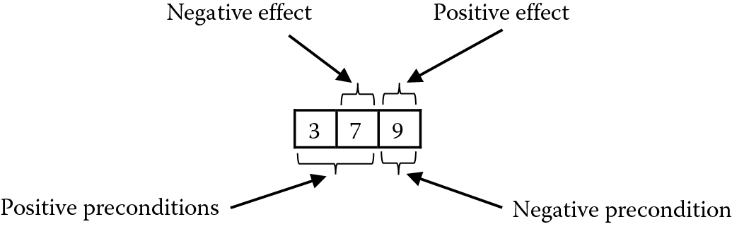
Three predicates of the action Take . Based on the key in Figure 13.1 , this three-digit array can be decoded as a = 1, b = c = d = 2, and e = p = 3.
Second, consider the following initial state:
(:initial (at-c(loc1, c1) and at-c(loc1, c2)
and at-c(loc2, c3) and at-c(loc3, c4)
and at-o(loc1, o1) and at-o(loc1, o3)
and at-o(loc3, o4) and at-o(loc5, o2)
and at-o(loc5, o5))
)
For instance, the action represented by the action signature Take(loc1,c1,o1) can be applied to the initial state because all its preconditions are satisfied in the initial state. But there are four more actions that can be applied to this initial state, represented by the four following action signatures: Take(loc1,c1,o3), Take(loc1,c2,o1), Take(loc1,c2,o3), and Take(loc3,c4,o4).
We can first note that each positive precondition identifier must match at least one state predicate identifier. Second, we can note that no state predicate identifier can be a negative precondition identifier. When these two quick tests pass, we can further test the applicability of an action, pushing further the use of the predicate identifiers.
To test the applicability of action Take in any state and in particular in the initial state earlier, we can sort the predicates of the state according to their identifier (refer to Figure 13.2). It is consequently possible to test only 20 pairs (4 instances of at-c × 5 instances of at-o) of predicates from the initial states instead of the 36 pairs (choosing any two elements in a set of 9 elements = (9 × 8)/2 = 36 pairs), which can be built from the initial state.
In Figure 13.3, the top array containing three and seven represents the positive preconditions of action Take. We then iterate over the predicates of the initial state. If an initial state predicate has the same predicate identifier as a precondition predicate, then this initial state predicate is pushed at the back of the appropriate column. If the identifier of an initial state predicate does not correspond to any identifier of a precondition predicate, then this initial state predicate is ignored. Finally, iterating in both columns, we can make pairs of predicates as indicated in Figure 13.3.
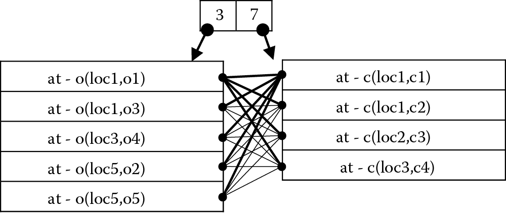
Note that if the language of the actions file allows predicates with the same identifier but with a different number of parameters, then the number of parameters must also be checked to build both columns in Figure 13.3.
There are various ways of achieving the iterations over both columns. For instance, we begin by forming the two-digit number made by the size of the columns in Figure 13.3: 54. Then we start with the two-digit value 00 and increase the rightmost digit; when this value reaches 4, we rewrite the two-digit number to 10 and increase it until the rightmost digit reaches 4 again. We then rewrite this number to 20 and so on until 54 is reached. This procedure builds the following list of two-digit numbers: 00, 01, 02, 03, 10, 11, 12, 13, 20, 21, 22, 23, 30, 31, 32, 33, 40, 41, 42, and 43. Alternatively, we can start from 43 and decrease until 00 is reached, thus producing the two-digit numbers of the previous list in the reverse order. Each of these 20 two-digit numbers can be used to access a position in both columns in order to make a pair of state predicates. The iterating procedure in Listing 13.1 works for any number of positive preconditions.
13.4.2 Recording Where the Action Parameters Occur in the Action Predicates
The procedure in Listing 13.1 generates tuples such that each state predicate identifier matches the identifier of a precondition predicate. Consequently, the unification procedure need only checking whether the state predicate parameters unify with the action parameters.
We know from Figure 13.3 that the positive precondition predicate whose shared position is 3, that is, at-o(?l,?o), is unified with state predicate at-o(loc5,o5), and then the parameter ?l of action Take gets the value loc5, and the parameter ?o of action Take gets the value o5. The positive precondition predicate whose shared position is 7, that is, at-c(?l,?c), with the parameter ?l equal to loc5, must now unify with state predicate at-c(loc3,c4). This fails because loc3 is different from loc5.
The idea is to record all the positions where an action parameter occurs in positive precondition predicates and then check that the parameters at these positions in the state predicates have the same value. For instance, the parameter ?l of action Take occurs as the first parameter of both positive precondition predicates. If the values at these positions in the state predicates are equal (which can be trivially achieved by testing the value of the first position against all other positions), then we can check for the equality of the occurrences of the next parameter. Recording the positions can be achieved once for all when parsing the action files.
13.5 Conclusion
A Visual C++ 2013 project is available from the book’s website (http://www.gameaipro.com), which implements a practical planner with the features (i.e., actions as text files and forward breadth-first search) and the data structures and algorithms described in this chapter.
Although planning is known to be very hard in theory, even the simplest planning algorithm can be implemented in a practical planner, which can be used for your gaming purposes, providing you focus on shrinking both memory and runtime requirements. Quick runtime and memory measurement routines, as well as relevant testing and systematic profiling, can hopefully help you succeed in making planning practical for your gaming purposes.
References
[Berger 14] Berger, E. 2014. The hoard memory allocator. http://emeryberger.github.io/Hoard/ (accessed May 26, 2014).
[Cheng 05] Cheng, J. and Southey, F. 2005. Implementing practical planning for game AI. In Game Programming Gems 5, ed. K. Pallister, pp. 329–343. Hingham, MA: Charles River Media.
[Deus Ex 3 DC 13] Deus Ex Human Revolution—Director’s Cut. Square Enix, 2013.
[F.E.A.R. 05] F.E.A.R.—First Encounter Assault Recon. Vivendi Universal, 2005.
[Garey 79] Garey, M. and Johnson, D. 1979. Computers and Intractability: A Guide to the Theory of NP-Completeness. New York: W.H. Freeman & Co Ltd.
[Ghallab 04] Ghallab, M., Nau, D., and Traverso, P. 2004. Automated Planning: Theory and Practice. San Francisco, CA: Morgan Kaufmann.
[IPC 14] International Planning Competition. 2014. http://ipc.icaps-conference.org/ (accessed May 28, 2014).
[Isensee 03] Isensee, P. 2003. Custom STL allocators. In Game Programming Gems 3, ed. D. Treglia, pp. 49–58. Hingham, MA: Charles River Media.
[Josuttis 13] Josuttis, N. 2013. The C++ Standard Library. Upper Saddle River, NJ: Pearson Education.
[Lazarov 08] Lazarov, D. 2008. High performance heap allocator. In Game Programming Gems 7, ed. S. Jacobs, pp. 15–23. Hingham, MA: Charles River Media.
[Lea 12] Lea, D. 2012. A memory allocator (2.8.6). ftp://g.oswego.edu/pub/misc/malloc.c (accessed May 26, 2014).
[Lung 11] Lung, R. 2011. Design and implementation of an in-game memory profiler. In Game Programming Gems 8, ed. A. Lake, pp. 402–408. Boston, MA: Course Technology.
[Masmano 08] Masmano, M., Ripoli, I., Balbastre, P., and Crespo, A. 2008. A constant-time dynamic storage allocator for real-time systems. Real-Time Systems, 40(2): 149–179.
[Noble 01] Noble, J. and Weir, C. 2001. Small Software Memory: Patterns for Systems with Limited Memory. Harlow, U.K.: Pearson Education Ltd.
[Orkin 04] Orkin, J. 2004. Applying goal-oriented action planning to games. In AI Game Programming Wisdom 2, ed. S. Rabin, pp. 217–227. Hingham, MA: Charles River Media.
[Rabin 00] Rabin, S. 2000. Real-time in-game profiling. In Game Programming Gems, ed. M. DeLoura, pp. 120–130. Boston, MA: Charles River Media.
[Rabin 11] Rabin, S. 2011. Game optimization through the lens of memory and data access. In Game Programming Gems 8, ed. A. Lake, pp. 385–392. Boston, MA: Course Technology.
[Tomb Raider 13] Tomb Raider—Definitive Edition. Square Enix, 2013.
[Wilhelm 08] Wilhelm, D. 2008. Practical logic-based planning. In AI Game Programming Wisdom 4, ed. S. Rabin, pp. 355–403. Boston, MA: Course Technology.