
Chapter 30
Modular Tactical Influence Maps
Dave Mark
30.1 Introduction
A large portion of the believability of AI characters in shooter and role-playing games (RPGs) comes from how they act in their environment. This often goes beyond what the character elects to do and gets into where the character decides to do it. Certainly, technologies such as traditional pathfinding and automatic cover selection provide much of this illusion. However, there is another layer of “spatial awareness” that, by helping to inform the decision process, can provide even more of the appearance of intelligence in game characters. Much of this stems from the character not only being aware of the static environment around it (i.e., the fixed level geometry) but also being aware of the positioning of other characters—both enemy and ally—in their immediate area. This is often done through the use of influence maps.
Influence mapping is not a new technology. There have been many articles and lectures on the subject [Tozour 01, Woodcock 02]. This article does not give a complete overview of how to construct and use them. Instead, we present an architecture we developed for easily creating and manipulating influence maps in such a way that a variety of information can be extracted from them and used for things such as situation analysis, tactical positioning, and targeting of spells. Additionally, while influence maps can be used on a variety of scales for things such as strategic or ecological uses—for example, the positioning of armies on a map or guiding the habitats and migrations of creature—this article will primarily focus on their use in tactical situations—that is, positioning in individual or small group combat. Note that many of the techniques, however, can be adapted for use in higher level applications.
This architecture was originally developed for the prototypes of two large, online RPG games. However, it can apply to many types of games including first-person shooters, RPGs, or even strategy games where multiple agents need to appear aware of each other spatially and act in a cohesive manner in the game space.
The in-game results that we achieved from utilizing this architecture included the following:
- Positioning of “tank style” defenders between enemies and more vulnerable allies such as spellcasters
- Determining the relative threat that an agent was under at a given moment
- Determining safe locations to evade to or withdraw to
- Identifying and locating clusters of enemies for targeting of area of effect spells
- Identifying locations for placement of blocking spells between the caster and groups of enemies
- Maintaining spacing from allies to avoid agents “bunching up”
- Determining when there enough allies near a prospective target to avoid “piling on”
30.2 Influence Map Overview
Tactical influence maps are primarily used by individual agents to assist in making tactical and positional decisions in individual or small group combat. The influence map doesn’t actually provide instruction—it only provides information that is used by the decision-making structures of the agents. One particular advantage to using influence maps is that they can represent information that all characters could potentially have knowledge of. By calculating and storing this information once for all characters, it prevents the expensive and possibly redundant calculation of information by each individual agent. For example, an influence map that represents where people are standing in a room is information that could potentially be common knowledge to those people. By calculating it once and storing it for all to access as needed, we save the time that would be involved in each agent processing that information on its own. An additional benefit is that, although the decisions are still being made by the individuals, by using shared information about the battlefield, some sense of emergent group behavior can result.
While a simple (x, y, z) coordinate is sufficient for describing the location of an object or agent in a space, an influence map gives a coherent way of describing how that object affects that space—either at that moment or possibly in the near future. It helps to answer questions such as the following:
- What could it hit?
- How far could it attack?
- Where could it move to in the next few seconds?
- What is its “personal space?”
While some of these seem like they could be answered with a simple direction vector (and they can), the advantages gained by the influence map are realized when multiple agents are affecting the space. Rather than dealing with the n2 problem of calculating multiple distance vectors between agents, we can look at the influence map and determine where the combined influence is. Now we can ask group-based questions such as “what could they hit?” or “where is it crowded?”
Additionally, the questions needed by game agents are often not “where is this,” but rather “where is this not.” The questions now become
- Where can they not hit?
- Where can I not be reached in the next few seconds?
- Where will I not be too close to people?
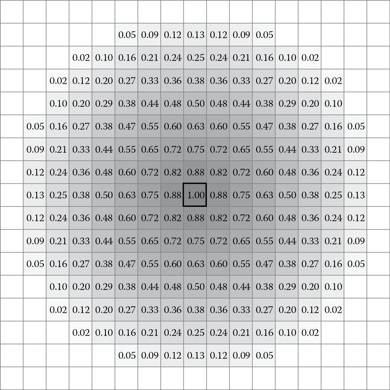
The basic form of the influence map is to divide the space into sections—most often a grid—and assign values to the cells. The values of the cells can represent a wide variety of concepts such as “strength,” “danger,” “value,” or anything else that can be measured. Typically, a value has a locus that the “influence” radiates out from. For example, an agent that has a certain strength in its local cell may radiate influence out to a certain radius with the influence declining as the distance from the agent increases (see Figure 30.1). In some implementations, this is the result of influence propagation that takes place over time. In our system, we simply evaluate the influence of individual cells as a function of distance from the locus.
In many implementations, including ours, when multiple agents are placed in an area together, the values that they radiate are added together so that a combined influence is created. By looking at the values of the cells, we can determine how much combined influence is in any given location. If the agents are closer together, the influence between them is higher than if they are farther apart. Because the influence decreases over distance, as you move away from the agents, you will eventually arrive at a location where their influence is 0. In Figure 30.2, you can see two agents who are close enough together that their influence overlaps. Note that, while each agent has a maximum influence of 1.0 (as in Figure 30.1), the area where they overlap significantly shows influences greater than 1.0.
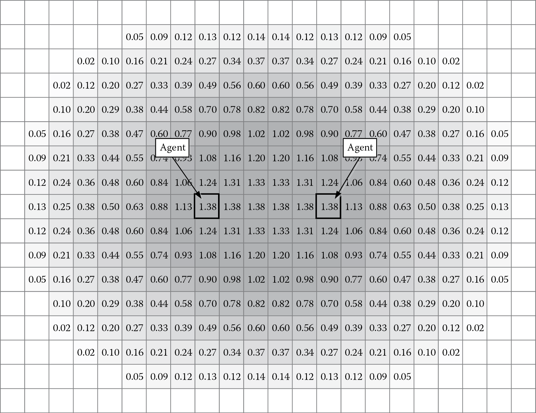
The combined influence from two agents can be greater than the influence of a single agent alone.
If the same process is performed for enemy agents and then inverted (i.e., allies are positive influence and enemies are negative), a topography is created that goes beyond a binary “ours” and “theirs.” It can also express ranges from “strongly ours” to “weakly ours” based on the total value in cells. The resulting map, such as the one in Figure 30.3, can give a view of the state of any given location on the map as well as the orientation of the forces in an entire area. Behaviors can then be designed to take this information into account. For example, agents could be made to move toward the battlefront, stay out of conflict, or try to flank the enemy.

An allied agent spreading positive influence and an enemy one spreading negative influence can show a “neutral zone” where the influence crosses 0.0.
Other information can also be represented in influence maps. For example, environmental effects such as a dangerous area (e.g., due to a fire, a damaging spell, or a pending explosion) can be represented and taken into account by the game agents in the same way that they can process information about the location of other agents.
30.3 Propagation
As we have alluded to earlier, influence can be propagated into the map from each agent. One way of propagating influence into a map is to walk through the cells surrounding the agent. For each cell, the influence is determined by using the distance from the agent to the center of that cell passed through a response curve that defines the propagation decay of the distance. For example, the formula for linear propagation of influence is shown in the following equation:
(30.1)
Note that influence propagation does not have to be a linear formula. In fact, different types of influence propagation might be better represented by other response curves. Another common type is an inverse polynomial defined by a formula similar to the one shown in the following equation:
(30.2)
Figure 30.4 shows the difference between linear propagation, the polynomial formula earlier, and a similar one with an exponent of 4 rather than 2. The graph in Figure 30.4 shows both the positive and negative sides of the equation in order to illustrate the “shape” of the influence circle around the agent that would result from the different formulas—specifically, the falloff of the values as the distance from the agent increases.
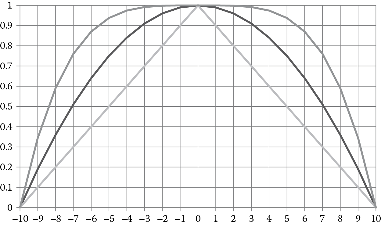
The shapes of a sample of propagation formulas centered on the agent: linear (inside) and two polynomial curves with exponents of 2 (middle) and 4 (outer).
The important thing to remember when selecting formulas is that the response curve simply shapes the propagation of the influence as it spreads away from the agent’s location. Note that there is nothing stating that the value must be at its maximum at the location of the agent. For example, a catapult is fairly innocuous at close range but has a ring of influence that it projects at its firing range. An influence map designed to represent this threat would be at its highest point in a ring surrounding the catapult rather than at its actual location.
All of the aforementioned propagations of threat assume no barriers to sight or movement around the agent. Certainly, that is not the case in many game environments. In those cases, other methods of propagation need to be employed. If the influence that is being spread is entirely based on line of sight (such as the threat from a guard or someone with a direct fire weapon), it is often enough to simply not propagate influence to locations that cannot be seen by the agent.
If the influence is meant to represent the potential threat of where an agent could possibly move—for instance, “what could that tiger bite in the next 3 seconds?”—the path distance between the agent and the location in question could be used. This helps solve situations where, for example, the tiger is on the other side of fence. Yes, it is close to the target location, but it is not a threat because it would take a while for the tiger to move around the fence. The solution here is often simply to swap the linear distance calculation code with a call to the pathfinding system to return a distance. Since many such queries are likely to be made over the course of an influence map evaluation, a common solution is to precompute cell path-distances for a large set of cells using an undirected Dijkstra search starting from the agent’s location. Either way, the costs in run-time performance and engineering effort alike are nonnegligible.
30.4 Architecture
There are different types of maps in our architecture. Some of them are the base maps for holding various types of information. Others are created at run time and stored for use in the repetitive task of populating the main maps. Still others are temporary in nature for use in combining the data into usable forms. The following sections describe each type of map.
30.4.1 Base Map Structure
The most important type of map structure is base map. The definition of this map is what determines the definitions of all the other maps to follow.
Maps are defined as rectangular areas so that they can be stored and accessed as a 2D array (or similar structure). The base map typically covers the entire level. In the case of maps where there are rigidly defined areas that are to be processed separately (e.g., the inside of a building), then a map could theoretically be smaller than the entire game level. It is often preferable, however, to attempt to simply combine maps into large areas due to complications of propagating influence from the edge of one map to an adjacent map. As you will see in the working maps section, it is usually easier to simply store the base map information in as large a chunk as possible.
Each map is a regular square grid. While the dimensions of the influence map are determined by the game map that it is to be used on, the cell granularity is more subject to adjustment. In general, they should be a size that would represent approximately the minimum granularity that you would want characters to position at, target at, etc. For example, if you want characters to “think in terms of” 1 m for where to stand, your cell sizes would be 1 m as well.
Because a small change in the granularity of cells can result in a massive change in the number of cells (and therefore the memory footprint and calculation time), a balance must be struck between the fidelity of the actions and the resources available to you. Suffice to say, there is no “right answer” for any of these values. They will have to be chosen based on the game design and the restrictions on processing power that might be in place.
30.4.2 Types of Base Maps
We use two types of base maps in our game. The first, and most common, is a map representing the physical location of characters—what we call a “proximity map,” or simply “prox map.” This map goes beyond showing the physical location at the moment—the influence radiated by the agents also shows where that agent could get to in a short period of time. Therefore, each agent’s presence in the location map is represented by a circle, centered on their current location and spreading out in a circle of decreasing value until 0 is reached (see Section 30.4.3). A proximity map that contains multiple agents would show not only their current locations but also where those agents could reach in short order. The higher the value of a cell, the closer that cell is to one or more agents and the higher the likelihood of it being influenced by an agent.
The second type of map is the “threat map.” This differs from the location map in that it represents not where an agent could go, but what it could potentially threaten. This may differ significantly depending on the game design. A game that involves only melee combat may have a significantly different set of demands for a threat map from a game involving gunfire with unlimited (or at least functionally unlimited) ranges. As we will see in the next section, the architecture supports different ranges of threat in the same game.
In the case of a melee unit, the threat map functions in a manner similar to the proximity map earlier, with the highest threat value propagated from the agent at the agent’s location and with the threat decreasing with distance to zero. In the case of ranged units, the threat influence may take the form of a ring of influence surrounding the agent’s location, as in the catapult example cited earlier. If a cell is being threatened by more than one agent, it is possible (even likely) that the threat value at that location will be greater than that generated by a single agent alone.
There will be one base map of each type (proximity and threat) for each faction in the game—often at least two factions (i.e., “us vs. them”). This allows us to pull information about either enemies or allies and combine them as necessary.
30.4.3 Templates
One problem with the calculation of influence propagation is the significant number of repetitive calculations that are needed. While they may seem trivial at first, we will soon realize that the calculations mount quickly as the number of agents increases. The most obvious fix is to limit the number of cells filled by only calculating cells in the square defined by our propagation radius. That is, if the radius of influence is 10 cells, only attempt to propagate into the cells that are within 10 vertically or horizontally from the agent—there’s no point in iterating through the potentially hundreds or thousands of cells that are outside that range. However, the major stumbling block is that the distance calculations between cells—even in the small area—involve many repetitive square root calculations. When multiplied by dozens—or even hundreds—of characters, these calculations can be overwhelming.
The best optimization that eliminates the repetitive distance and response curve calculations is gained through the use of “templates.” Templates are precalculated and stored maps that can be utilized by the influence map engine to “stamp” the influence for agents into the base map. We precalculate and store templates of various sizes at start-up. When it comes time to populate the map (see Section 30.5), we select the appropriate size and type of map and simply add the precalculated influence values in the template into the map at the appropriate location. Because the propagation has already been calculated in the template, we eliminate the repetitive distance and response curve calculations and replace them with addition of the value of the template cell into a corresponding cell on the base map.
As we alluded to earlier, this “stamp” method does not work when there are significant obstacles to movement in the area—particularly for proximity maps. For those situations, it would be necessary to calculate the path distance and then determine the influence value for that location.
The number and type of templates that we need depends on a number of factors:
- What does the base map represent?
- What is the possible range of values that we would use to look up the correct template?
- What is an acceptable granularity for that range of values?
As we go through the three types of templates, we will see how these values determine how many templates we need and what they represent.
Note that the influence in each of these templates is normalized—that is, the range of values is between 0 and 1. This is largely because we are defining the shape of the influence curve only at this point. When it comes to usage of the templates, we may often use these simple normalized curves. However, as we will explain shortly, we may want to multiply the “weight” of the influence that an agent has. By leaving the templates normalized, we can make that decision later as needed.
We utilize two different types of templates—one for proximity maps and one for threat maps. We use different templates because the propagation formula differs between them. If we were using the same formula, the templates would be identical and this differentiation would not be needed.
The first type of template is used for location maps. A location template represents what was discussed earlier in this article—where can the agent get to quickly? As mentioned in the propagation section earlier, the formula for location templates should be a linear gradient with a formula as shown in Equation 30.1.
If our map granularity was 1 m (meaning a cell was 1 m2), our maximum speed in the game was 10 m/s, and our refresh time on maps was 1 second, and our maximum map size would be a radius of 10 m. This allows us to propagate influence out to how far an agent could get in the amount of time between map updates (1 s). Therefore, our maximum template size would be a 21 × 21 grid (10 cells on either side of the center row or column).
In order to support agents that would move at slower speeds, we must create templates that radiate out to different ranges, however. If there was a slower agent that only moved at 5 m/s, we would need one for that speed. In an RPG where there could be many different types of characters with many different movement speeds, we may want to have 1 template for each integer speed from 1 to 10.
Constructing templates for threat maps—the second type of template—would be similar. However, there are a couple of changes. First, threat maps are best calculated with a polynomial formula that reflects that the threat is similar across most of the distance and only drops off as it reaches its furthest point. Equation 30.3 shows a formula that we often use for this—a polynomial with an exponent of 4:
(30.3)
The template is looked up by using the maximum range of the threat of the agent. An RPG character with a spell range of 30 m, for example, would need a map that was 61 × 61. On the other hand, a primarily melee character with a range of 2 m would use a significantly smaller map.
As with the speeds earlier, there needs to be a map that approximately matches the threat range of the agent in question. If you have only a small number of very specific characters and abilities, then certainly create templates to match. If there is a wider variety that would necessitate more sizes of maps, use discretion in how to create them. Because of the potentially great variety and differences between threat ranges, it might not be advisable to create one template for each measurement unit (in our example, each meter). Instead, templates can be created at specified intervals so as to give coverage adequate enough to provide a template that is at least roughly similar to the needs of the agent.
The third type of template is the personal interest map. Rather than being used to propagate influence into the base maps, these templates are specifically designed to apply to other maps in order to determine what an agent might be interested in. We will discuss the application of these maps later. As with location and threat templates, depending on the game design, it is often advisable to have multiple sizes of these maps as well so the appropriate size can be applied as needed without calculation.
30.4.4 Working Maps
Working maps are temporary maps that are used to assemble data from the main maps and templates. Working maps can be of any size but they are usually smaller than the main map because they only are used for the data directly relevant to a decision. They will always be as large as the largest template used for the decision. Most often, the working maps will be centered on the agent location (Figure 30.5).
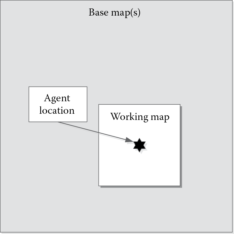
A working map is a temporary, small map centered on an agent used to assemble and process information from multiple maps in the local area.
The rationale behind working maps is that, when we are assembling combinations of map information, we will often be iterating over the relevant portions of the required maps to add or multiply their values. There is no point in iterating over the entire level if we are only interested in values that are close to the agent requesting the information. By creating a working map and copying the necessary values from the base maps into it (through addition or multiplication), we limit the iterations necessary and the memory footprint needed.
Because working maps are discarded immediately after use, in a single-threaded environment, there will only be one working map in existence at a time. In order to eliminate the issue of repeatedly creating and destroying these arrays often, it is often a good idea to create a single, larger, working map and preserve it for continual use.
30.5 Population of Map Data
Because the base maps must draw their information from the world data—namely, the positions and dispositions of the agents—they must be updated on a regular basis. For the games we have used this system on, we updated tactical influence maps once per second. However, any frequency can be selected based on the needs of the game, the period between think cycles for your agents, and the processing power available. For tactical movement, we would not recommend updating them any faster than 0.5 s (game characters will not need data much faster than that) or any less often than every 2 s (the data will get too stale between updates).
On each update, the map is first zeroed out—no data is carried over from one pass to the next. We then iterate through the population of the game world, and, for each agent, we apply—or “stamp”—their influence onto the appropriate maps for their faction based on their location. Assuming that we are using both proximity and threat maps, this means that each character is registering its influence on the two maps corresponding to its faction.
For the proximity map, we select the proximity template that most closely corresponds to the agent’s maximum speed. That is, if an agent’s maximum speed was 4 m/s, we would select the template that matched this. (If we had used integer speeds from 1–10, this would simply be the template for a speed of 4.) We then align the center of the template with the corresponding cell on the base map, offset by the size (in cells) of the template, and add the cell values from the template into the base map.
Looking up the appropriate threat template is similar to the process for the location templates earlier. As mentioned in the section on creating and storing templates, however, there may be more “slush” in selecting the correct sized template. Whether you round up or down is purely a game design decision. Rounding up to a larger threat template will cause their ranges to seem bigger than they are—possibly making attackers stay farther away. On the other hand, rounding down may cause attackers to seem that they don’t realize the danger of the agent that is projecting the threat. Regardless, once the appropriate template is selected, the process of applying it into the base map is identical.
Note that in both cases, care must be taken along the edges of the map. If an agent is closer to the edge of map than the radius of its template, the addition process will attempt to apply the value of the template cell to a base map cell that does not exist. This is avoided simply by range checking on the bounds of the base map cells.
One possible addition to this process is that we may want different agents to exert different levels of influence into the map. For example, a weak character with a threat range of 10 needs to be represented differently than a strong character with an identical threat range. We need a representation that the area around the stronger character is more dangerous than around the weaker character.
Because the templates are normalized to 1.0, we can simply add a magnitude to the process of adding the influence to the map. If the stronger character was three times as powerful as the weaker character, we would simply need to pass a strength value of 3 into the function and the values in the template would be multiplied by 3 as it is stamped into the threat map. Therefore, the value of the influence of the stronger character would start at 3 and drop to 0 at the maximum range.
30.6 Information Retrieval
Once information is in the base maps, it can be retrieved in different ways depending on the needs at the time. While we will address specific use cases in the next section, the process is the same for most applications.
30.6.1 Values at a Point
The simplest form of information is retrieving the value of one map or a combination of maps at a specified point. For example, if an agent wanted to know the amount of enemy threat at its location, it could simply retrieve the value of the threat map cells for each faction that it considers an enemy. These are simply added together and returned to the agent for its consideration. Again, more use cases will be covered in the next section.
30.6.2 Combinations of Maps
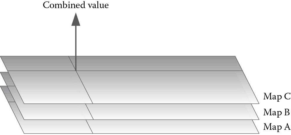
Much as we applied templates into the base maps, we can lift information out of the base maps into working maps. The process is essentially the reverse of how we applied templates into the base map. We do this so that we can easily combine the map information for the area of interest without having to worry about processing the entire map.
In addition to simply passing the map into the functions to be modified, we also can pass in a modifier that dictates a magnitude for the modification. For example, rather than simply constructing a working map that consists of the values in MapA plus the values in MapB, we can specify that we want the values in MapA plus 0.5 times the values in MapB. The latter would yield a different output that might suit our purposes better at the time. In words, it would read “the influence of MapA plus half of the influence of MapB.” By doing so, we can craft “recipes” for how an agent is looking at the world—including priorities of what is important to consider.
By including basic functions for adding and multiplying maps into the map class, we can construct a simple syntax that assists in building a working map that includes the information that we need. Each function takes a map and processes it into the working map according to its design and parameters if necessary. This is how we achieve the modularity to be able to construct a variety of outputs in an ad hoc manner.
For example, our code could look like the following:
WorkingMap.New(MyLocation);
WorkingMap.AddMap(EnemyLocationMap(MyLocation), 1.0f);
WorkingMap.AddMap(AllyLocationMap(MyLocation), -0.5f);
WorkingMap.MultiplyMap(InterestTemplate(MyLocation), 1.0f);
Location InterestingPlace = WorkingMap.GetHighestPoint();
We will see what can be done with these combinations in the next section.
30.6.3 Special Functions
There are a number of special functions that we must set up in order to make things easier for modular use later.
First, we can construct a general “normalization” function that takes a working map and normalizes its values to be between 0 and 1. The standard method of normalizing is to take the highest and lowest values present on the map and scale the contents such that they become 1.0 and 0.0, respectively. For instance, consider a map with a maximum value of 1.4 with a particular cell that had a value of 0.7. After normalization, the maximum value would be 1.0 (by definition) and the cell in question would now have a value of 0.5 (0.7/1.4).
The normalized map is convenient for times when we are interested in the general “terrain” of the map, but not its true values. We can then take that normalized map and combine it meaningfully with other normalized maps. We will investigate those further in the next section.
The other helper function is “inverse.” In this case, we “flip the map contours upside down” in effect. This is done by subtracting the cell values in the map from 1.0. Therefore, an influence map of agents that would normally have high values at the points of greatest concentration and 0 values at the locations of no influence would now have a value of 1.0 at the places of no influence and its lowest points at the locations of the greatest influence.
The inverse function is helpful when combining maps from enemy factions. Instead of subtracting one faction’s map from another, we can add one map to the inverse of the other. While, at first glance, this seems like it would yield the same result, the shift in values allows us to preserve convenient functions (such as retrieving the highest point) in our modular system.
30.7 Usage
The collection and storage of influence map data is useless without ways to use it. The power of the system is in how many ways the underlying data can be reassembled into usable forms. This information retrieval and processing can be divided into three general categories:
- Gathering information about our location and the area around us
- Targeting locations
- Movement destinations
We address each of these in Sections 30.7.1 through 30.7.3.
30.7.1 Information
The most basic function that the influence map system can serve is providing information about a point in space. One function simply provides an answer to the simple question, “what is the status of this point?” The word “status” here could mean a wide variety of things depending on the combination of maps utilized in the query. However, other methods can query an entire area and answer the similar question, “what is the status of the (highest/lowest) point around me?” The latter can be done without specifying a point at all simply by looking at the surrounding area.
The first method—that of querying a specific point—is achieved by querying the value of a location through its associated influence map cell on one or more maps (Figure 30.6). For example, if we wanted to know the total threat from our enemies at the location we are standing, we would simply retrieve the value of the cell we are standing in from all of the threat maps that belong to enemy factions. Because the value that is returned represents the total threat at our location, it can be used in decisions such as when to relocate to a safer position. A similar query of the physical proximity map of our own faction would hint us as to whether or not we might need to move slightly to give space to our co-combatants. Note that this method does not require us to use a working map because we are only interested in the values of individual cells.
We can query a point on the map and retrieve data accumulated from a combination of maps at that point.
Another method for querying information is to look at the entire area surrounding us. For example, we may want to query the area to see if there are concentrations of enemies that are standing close together. To do this, we create a working map that is the same size as a personal interest template that, in this instance, might be how far we could attack in 1 s (our maximum threat range + our movement speed). We then populate that working map with the data from the proximity maps of our enemies. We then run a function that walks through the working map and returns the highest value (not the location). This value tells us what the maximum concentration of enemies is due to the fact that enemies closer together have their influence areas overlapping resulting in a higher sum as is shown in Figure 30.7. This might be useful in informing us that we might want to cast an area of effect spell. (Note that the location at which we would cast it is addressed in the next section.)
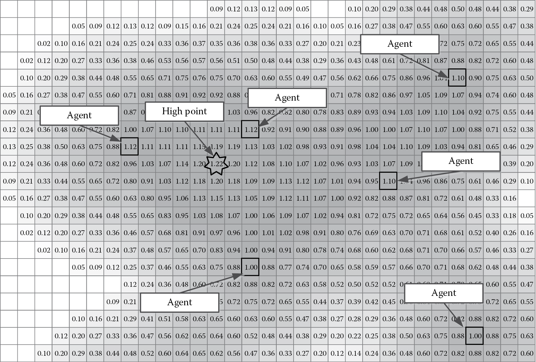
The “center of mass” of agents can be determined by finding the highest value on one or a combination of base maps.
The usefulness of the modular nature of the map system becomes clear when we extend the aforementioned query to ask, “what is the highest concentration of all factions?” We could add all the factions together and find the highest value. Summing the enemy factions to the inverse of allied factions would give a number representing the highest concentration of enemies that isn’t close to any allies. By mixing location and threat maps, we can extend the possible information we can get.
Often, it is good to prioritize information that is closer to the agent so that it doesn’t make decisions that cause it to, perhaps, run past one threat to get to another. By multiplying the resulting working map by our personal interest template, we adjust the data so that closer cells are left relatively untouched, but cells on the periphery are reduced artificially—ultimately dropping to zero. In the example shown in Figure 30.8, the high point on the original map (a) is located at the edge of the personal interest map (b) surrounding the agent’s location (dotted line). By multiplying the original map by the interest map, the resulting map (c) yields a different high point. While the actual value of this location is smaller than the high point in the original map, it is prioritized due to its proximity to the agent’s actual location. Note that any points outside the radius of the personal interest map are reduced to 0 due to multiplying by 0.This is similar to the agent saying, “Yes, there is something interesting over there, but it is too far away for me to care.”
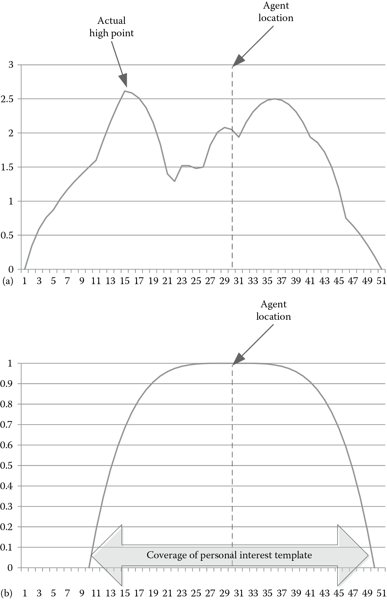
A complex influence map (a), when multiplied by a personal interest template (b),(Continued )
30.7.2 Targeting
Another primary use for assembling information from combined influence maps is for use in targeting. In the aforementioned section, we mentioned that we could query the local area for the highest value. By using a similar process, we can acquire the actual location of the cell that produced that value. This is as simple as making a note of the cell in the working map that contains the highest value and then converting it back into a position in the world.
Possible uses for this include using the proximity maps for determining a location to cast an area of effect spell—a damaging one against enemies or a healing buff for allies. By finding the highest point on the working map, we know that it is the center of concentration of the forces of the faction we are checking. This means that the target will not be a character in the world but rather at a point that should be the “center of mass” of the group. Referring again to Figure 30.7, the “high point” identified on the map is the location of the highest concentration of agents.
Because of the modular nature of the system, we could add the enemy location maps together and then subtract the location maps for allies. The resulting high point would give a location of concentration enemies that is also not near allies. This might be useful in avoiding friendly fire, for example.
Another possible use would be identifying a position between the agent and the bulk of the enemies or even between the bulk of the agent’s allies and the enemies. This might help identify where to place a blocking spell such as a wall of fire. This is accomplished by determining that point of the concentration of the enemies as we did earlier, but then using that as an endpoint for a line segment either between that point and the agent or that point and a corresponding one for the allies. In effect, this is determining the “threat axis” to be aware of. By selecting a location partway along that segment, you are able to identify a spot that would be good for a blocking spell (Figure 30.9) or for the positioning of forces, as we shall see in the next section.
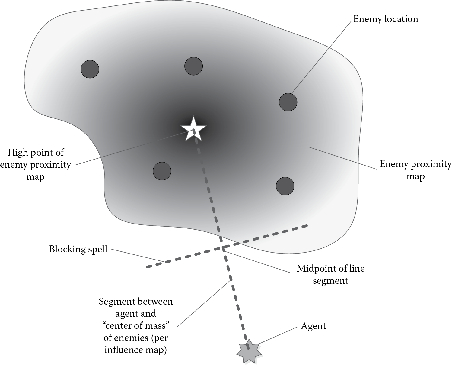
By determining the location of the high point of the enemy proximity map, we can select a location along the line between that point the agent to position a blocking spell, for instance.
30.7.3 Positioning
The third primary use for tactical influence maps is to inform movement commands. This is very similar to the use for targeting earlier. Upon deciding that it would like to perform some sort of movement (move toward a group, withdraw to a safe spot), the agent requests an appropriate destination location from the influence map system. As with the methods earlier, a working map is created and populated with data from the necessary maps, the personal interest template is applied (via multiplication), and the highest or lowest scoring location is returned.
Another use for positioning is to encourage spacing between agents—notably allied agents. By subtracting the location maps of the agent’s faction—and adding the agent’s own proximity template—the agent can adjust and take allied agents’ positioning into account. This can be used on a stand-alone basis for a simple “spacing” maneuver (e.g., as part of an idle) or as a modifier to other positioning activities. At this point, the logic from the influence map request can be read as something similar to “find me a location that is away from enemy threats but also spaced apart from my allies.”
30.8 Examples
The following are some examples of modularly constructed influence maps that can be used for common behaviors. Note that this assumes only one enemy and one allied faction. A separate code could be written to assemble all relevant factions.
The examples are written in a simplified structure for brevity and clarity. The actual implementation of the functions referenced here would be more involved and would differ largely depending on your base implementation. However, the actual modular functions to access the data should be little more complicated than what is shown here.
30.8.1 Location for Area of Effect Attack
This identifies if there is a point that is worth casting an area of effect attack on and retrieves the location. The MultiplyMap function that applies the InterestTemplate (of a size determined by our movement speed) is used to prioritize locations that are closer to the agent similar to what is show in Figure 30.8.
WorkingMap.New(MyLocation);
WorkingMap.Add(LocationMap(MyLocation, ENEMY), 1.0f);
WorkingMap.Multiply(InterestTemplate(MySpeed), 1.0f);
return WorkingMap.GetHighestLocation();
Note that to change the aforementioned code to find a position for an area of effect spell for allies (such as a group buff spell), we only would need to change the parameter ENEMY to ALLY.
30.8.2 Movement to Safer Spot
This identifies the location near the agent that has the least amount of enemy physical influence. This is good for finding a location for the character to move that is away from the immediate physical range of enemies.
WorkingMap.New(MyLocation);
WorkingMap.AddInverse(LocationMap(MyLocation, ENEMY), 1.0f);
WorkingMap.Multiply(InterestTemplate(MySpeed), 1.0f);
return WorkingMap.GetHighestLocation();
By using the inverse of the enemy location map, we are saying that the places where the cell values are low (or even 0)—that is, away from enemies—are now the highest points. Correspondingly, the highest points on the map are now the lowest due to the inverse. Since we are looking for place with the fewest enemies, we now can use the GetHighestLocation() function. Of course, the highest points would be modified somewhat after the application of the interest map, again as visualized in Figure 30.8.
Note that this code can also be used for moving away from allies (e.g., to keep spacing) simply by changing the parameter ENEMY to ALLY.
Additionally, by changing the code to use the threat map of enemies, we could find a location that had the least amount of enemy threat (but was also close to our location by application of the interest template). The new code would be as follows:
WorkingMap.New(MyLocation);
WorkingMap.AddInverse(ThreatMap(MyLocation, ENEMY), 1.0f);
WorkingMap.Multiply(InterestTemplate(MySpeed), 1.0f);
return WorkingMap.GetHighestLocation();
30.8.3 Nearest Battlefront Location
To determine a location that is in the area between our allies and our enemies, we multiply the enemy threat map by the ally threat map. The resulting map has high points along a line where the two maps overlap the most (Figure 30.10). By further multiplying this map by the interest template, we can find a location nearest to the agent that is “on the front lines.”
Multiplying enemy threat (or location) by ally threat (or location) yields high points along the front lines.
WorkingMap.New(MyLocation);
WorkingMap.Add(ThreatMap(MyLocation, ENEMY), 1.0f);
WorkingMap.Multiply(ThreatMap(MyLocation, ALLY), 1.0f);
WorkingMap.Multiply(InterestTemplate(MySpeed), 1.0f);
return WorkingMap.GetHighestLocation();
As we noted in the prior section, by subtracting our ally’s proximity, we can find a point that is “on the front” but also away from our fellows. This leads to a behavior where allied agents will spread out along a battlefront by selecting a location that is not only in between the bulk of allies and enemies but also physically apart from their comrades. In order for this to work, we need to normalize the result of the map earlier and then subtract a portion of the ally proximity map. The version of the ally proximity map that we need must not include our own proximity. Therefore, a function is created that returns the ally proximity without our own information. This would simply be as follows:
AllySpacingMap.New(MyLocation);
AllySpacingMap.Add(LocationMap(MyLocation, ALLY), 1.0f);
AllySpacingMap.Add(LocationTemplate(MyLocation, MySpeed), -1.0f);
Return AllySpacingMap&();
We can then apply this spacing map into our original formula. The adjusted code would read as follows:
WorkingMap.New(MyLocation);
WorkingMap.Add(ThreatMap(MyLocation, ENEMY), 1.0f);
WorkingMap.Multiply(ThreatMap(MyLocation, ALLY), 1.0f);
WorkingMap.Normalize();
WorkingMap.Add(AllySpacingMap(), -0.5f);
WorkingMap.Multiply(InterestTemplate(MySpeed), 1.0f);
return WorkingMap.GetHighestLocation();
Note that we are multiplying the ally spacing map by a scaling factor of 0.5 before we subtract it in order to make it less of an impact on the positioning than the battlefront itself.
30.9 Conclusion
As we have demonstrated, influence maps can be a powerful tool for agents to understand the dynamic world around them. By providing a modular system that allows programmers to combine individual map components in a variety of ways, a wide variety of expressivity can be easily created and tuned with relative ease.
References
[Tozour 01] Tozour, P. 2001. Influence mapping. In Game Programming Gems 2, ed. M. DeLoura, pp. 287–297. Charles River Media, Hingham, MA.
[Woodcock 02] Woodcock, S. 2002. Recognizing strategic dispositions: Engaging the enemy. In AI Game Programming Wisdom, ed. S. Rabin, pp. 221–232. Charles River Media, Hingham, MA.