
Chapter 19
Guide to Anticipatory Collision Avoidance
Stephen J. Guy and Ioannis Karamouzas
19.1 Introduction
Anticipation is a key aspect of human motion. Unlike simple physical systems, like falling rocks or bouncing balls, moving humans interact with each other well before the moment of actual collision. This type of forethought in planning is a unique aspect to the motion of intelligent beings. While physical systems (e.g., interacting electrons or magnets) show evidence of oriented action at a distance, the intelligence humans show in their paths is a unique phenomenon in nature, and special techniques are needed to capture it well.
In games, the act of computing paths that reach a character’s current goal is typically accomplished using some form of global planning technique (see, e.g., [Snook 00, Stout 00]). As a character moves along the path toward its goal, it still needs to intelligently react to its local environment. While, typically, there are not computational resources available to plan paths that account for every local detail, we can quickly modify a character’s path to stay free of collisions with any local neighbors. In order to keep this motion looking realistic and intelligent, it is important that our characters show clear anticipation even for this local collision-avoidance routine. Consider, for example, the scenario shown in Figure 19.1, where two agents pass each other walking down the same path. On the left, we see the result of a last second, “bouncy-ball” style reaction—the characters will get to their goals, but the resulting motion does not display much anticipation. In contrast, the right half of the figure shows our desired, humanlike behavior, where characters are able to anticipate the upcoming collision and efficiently adapt their motions early on.
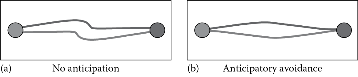
(a) Simple reactive agents versus (b) anticipatory agents. Anticipatory agents exhibit smooth and efficient motion as compared to simple reactive agents.
In this chapter, we will present the key ideas needed to implement this type of high-quality, anticipatory collision avoidance for characters in your game. After explaining the main concepts, we will provide a step-by-step explanation of a modern anticipatory collision-avoidance algorithm and discuss how to optimize its implementation. We will also walk through the approaches taken by modern systems used in commercial games and explain how they relate to the algorithm presented here.
19.2 Key Concepts
Before presenting our avoidance model, we need to cover some key foundational concepts. The collision-avoidance system we describe here is agent based. This means that each animated character a user may encounter in the current scene, no matter how complex, is described by a simple abstract representation known as an agent. Each agent has a few variables that store the state of the corresponding animated character. The exact variables used will vary from different implementations, but common agent states include position, velocity, radius, and goal velocity.
Each agent is expected to update its state as part of a larger game loop. We assume that each agent has an individual goal velocity that represents its desired speed and direction of motion, typically set by external factors such as an AI planner or a player’s input. Each time through the game loop, our task will be to compute collision-avoidance behaviors for each agent. The approaches we will discuss are anticipatory, updating the positions of each agent by finding new velocities that are free of all upcoming collisions. In the following, we detail each variable in the agent state and give complete code for quickly determining if two agents are on a collision course.
19.2.1 Agent State
Listing 19.1 provides the complete state of each agent. Each variable is stored as an array across all the agents.
- Radius (float): We assume that the agent moves on a 2D plane and is modeled as a translating disc having a fixed radius. At any time, the center of the disc denotes the position of the agent, while the radius of the disc defines the area that is occupied by the agent and that other agents cannot step into. By choosing a larger disc than the one defined by the shoulder–shoulder distance of the animated character, we can allow larger separation distances between agents while they pass each other. In contrast, if the radius is smaller than the visualization radius, the animation engine should be able to account for such a difference (e.g., by rotating the upper body).
- Position (2D float vector): A simple 2D vector of the agent’s x and y position is needed to locate the agent.
- Velocity (2D float vector): The agent moves across the virtual world with a certain velocity. In the absence of any other agents, this velocity is the same as the goal velocity. Otherwise, the agent may have to adapt its current velocity to ensure a collision-free navigation.
- Goal velocity (2D float vector): At any time instant, the agent prefers to move toward a certain direction at a certain given speed. Together, these two components define the agent’s goal velocity (for instance, a velocity directed toward the agent’s goal having a unit length). In most games, the goal velocity is passed to the agent by a global navigation method or directly by the player.
19.2.2 Predicting Collisions (Time to Collision)
To exhibit intelligent avoidance behavior, an agent must be able to predict whether and when it is going to collide with its nearby agents so that it can adapt its velocity accordingly. We can use the concept of a time to collision (denoted τ) to reason about upcoming interactions. Specifically, a collision between two agents is said to occur at some time τ ≥ 0, if the corresponding discs of the agents intersect. Consequently, to estimate τ, we extrapolate the trajectories of the agents based on their current velocities. Then, the problem can be simplified into computing the distance between the extrapolated positions of the agents and comparing it against the sum of the combined radii of the agents.
More formally, given two agents A and B, a collision exists if
(19.1)
Here, to estimate the extrapolated positions of the agents, we assume that the agents move at constant speed. Even though such an assumption does not always hold, it practically works very well for predicting and avoiding upcoming collisions, especially in the short run. Squaring and expanding (19.1) leads to the following quadratic equation for τ:
(19.2)
where
For ease of notation, let and Then, the aforementioned equation can be solved following the quadratic formula, allowing us to estimate the possible time to collision between the two agents: Note that since b is a factor of 2, by setting the solution can be simplified as , allowing us to save a couple of multiplications.
If there is no solution or only one (double) solution then no collision takes place and τ is undefined. Otherwise, two distinct solutions exist leading to three distinct cases:
- If both solutions are negative, then no collision takes place and τ is undefined.
- If one solution is negative and the other is nonnegative, then the agents are currently colliding, that is, τ = 0.
- If both solutions are nonnegative, then a collision occurs at
In practice, one does not need to explicitly account for all these cases. Assuming that the agents are not currently colliding, it suffices to test whether is nonnegative. Otherwise, τ is undefined. The code for computing the time to collision between two agents is given in Listing 19.2.
19.2.3 Time Horizon
It is typically not necessary (or realistic) for an agent to worry about collisions that are very far off in the future. To account for this, we can introduce the notion of a time horizon that represents the furthest out point in time after which we stop considering collisions. In theory, an agent can try to resolve all potential collisions with other agents that may happen in the future. However, such an approach is computationally expensive and unrealistic, since game-controlled avatars and NPCs can drastically change their behaviors well before the predicted collision happens. As such, given a certain time horizon (e.g., 3 s), an agent will ignore any collisions that will happen more than seconds from now. This not only reduces the running time but also leads to more convincing avoidance behavior.
Note that the time horizon can vary between agents, increasing the heterogeneity in their behaviors. An aggressive agent, for example, can be modeled with a very small time horizon (slightly larger than the time step of the simulation), whereas a large time horizon can be assigned to an introvert or shy agent. Some examples of varying the time horizon are shown in the following section.
19.3 Prototype Implementation
Armed with the concepts of agent-based simulations, goal velocities, time horizons, and an efficient routine to compute the time to collision between two agents, we can now develop a full multiagent simulation algorithm, complete with anticipatory collision avoidance between agents. After providing method details, and code, we’ll show some simple example simulations.
19.3.1 Agent Forces
At any given time, an agent’s motion can be thought of as the result of competing forces. The two most important forces on an agent’s path is a driving force, which pushes an agent to its goal, and a collision avoiding force, which resolves collision with neighboring agents in an anticipatory fashion. Typically, an agent’s driving force is inferred from its goal velocity. If the agent is currently moving at its desired direction and speed, no new force is needed. However, if the agent is moving too fast, too slow, or in the wrong direction, we can provide a correcting force that gradually returns an agent back to its goal velocity with the following equation:
(19.3)
where
is the agent’s goal velocity
k is a tunable parameter that controls the strength of the goal force
If k is too low, agents lag behind changes in their goal velocity. If k is too high, the goal force may overwhelm the collision-avoidance force leading to collisions between agents. In the examples later, we found that a k of 2 balances well between agents reaching their goal and avoiding collisions.
If an agent is on a collision course with any of its neighbors it will also experience a collision-avoidance force. The magnitude and direction of this avoidance force will depend on the predicted time until the collision and the expected point of impact, as detailed in the next section. The sum of all of the collision-avoidance forces from the agent’s neighbors along with the goal-directed driving force will determine the agent’s motion.
As part of the overall game loop, each agent performs a continuous cycle of sensing and acting with a time step, Δt. A time step begins with an agent computing the sum of all the forces exerted on it as outlined earlier. Given this new force, an agent’s velocity, v, and position, x, can be updated as follows:
(19.4)
which is a simple application of Eulerian integration, with the current force updating the agent’s velocity and the new velocity updating the agent’s position. A small time step, Δt, can help lead to smoother motion; in the examples later, we use a Δt of 20 ms.
19.3.2 Avoidance Force
Each agent may experience a unique avoidance force from each of its neighboring agents. Because this force is anticipatory in nature, it is based on the expected future positions of the agents at the time of collision rather than on the agents’ current positions. The avoidance force is computed in two steps with the direction of the avoidance force being computed separately from the magnitude.
19.3.2.1 Avoidance Force Direction
To compute the direction of the avoidance force, both agents are simulated forward at their current velocity for τ seconds. The direction of the avoidance force is chosen to push the agent’s predicted position away from its neighbor’s predicted position as illustrated by the gray arrows in Figure 19.2. By extrapolating an agent along their current velocity, the avoidance direction that an agent A experiences from a neighboring agent B can be computed efficiently as follows:
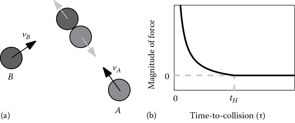
Computing the avoidance force. When agents are on a collision course an avoidance force is applied. (a) The direction of the force (gray arrows) depends on the relative positions at the moment of the predicted collision. (b) The magnitude of the force is based on how imminent the collision is (as measured by time to collision τ ).
(19.5)
19.3.2.2 Avoidance Force Magnitude
The magnitude of the avoidance force is inferred from the time to collision τ between the two agents. When τ is small, a collision is imminent, and a very large avoidance force should be used to prevent the collision. When τ is large, the collision will take place far in the future, and the avoidance force should have a small magnitude, vanishing to a value of zero at the time horizon There are many functions with these two properties. Here, we propose the function that is fast to compute and smoothly drops the force to zero as τ approaches (see Figure 19.2). This means the final avoidance force can be computed as
(19.6)
19.3.2.3 Corner Cases
If two agents are already colliding, the time to collision is zero, and the magnitude of the force is undefined. This condition can be quickly detected by comparing the distance between two agents to the sum of the radii. One option is to use a special nonanticipatory force to push colliding agents away from their current positions. In practice, we find the following simple trick to be sufficient: if two agents are colliding, shrink their radius for this one time step to just under half the distance between the agents. Most collisions between agents are quite small, and this will prevent the collision from getting any worse.
Additionally, agents who are very close and moving toward each other will have a very small time to collision. Following Equation 19.6, these agents will have very high (near infinite) avoidance forces that would dominate the response to all other neighbors. To avoid this, we can cap the maximum avoidance force to a reasonable value (we use 20 in the examples later).
19.3.2.4 Code
Listing 19.3 gives complete pseudocode implementing the collision-avoidance algorithm outlined in this section. The supplemental code corresponding to this chapter on the book’s website (http://www.gameaipro.com) provides complete python code for this algorithm, including a simple scenario where agents move with heterogeneous velocities and directions on a 2D plane.
19.3.3 Runtime Performance
The aforementioned algorithm is fast to compute, and optimized implementations can compute avoidance forces for thousands of agents per frame on modest hardware. The main bottleneck in performance is actually determining an agent’s neighbors. A naïve implementation might, for each agent, iterate over all other agents to see if they are on a collision course, resulting in quadratic runtime complexity. However, the pseudocode in Listing 19.3 illustrates a more efficient approach, pruning the search for nearest neighbors before computing any forces to only consider agents within a certain sensing radius (e.g., the distance that the agent can travel given its time horizon and maximum speed). The proximity computations in the pruning step can be accelerated using a spatial data structure for nearest neighbor queries, such as a k-d tree or a uniform grid. By selecting a fixed maximum number of neighbors for each agent, the runtime will be nearly linear in the number of agents.
19.3.4 Parameter Tuning
Any collision-avoidance method has tunable parameters that affect the behavior of the different agents. For example, agents with larger radii will move further away from their neighbors (perhaps looking more shy), and agents with a larger goal velocity will move faster (looking more hurried or impatient). For an anticipatory method, one of the most important parameters to tune is the time horizon, as it has a strong affect on an agent’s behavior.
Figure 19.3 shows the effect of varying the time horizon. In this scenario, every agent is given a goal velocity of moving in a random, predetermined direction at 1.5 m/s. With a very small time horizon of 0.1 s (Figure 19.3), agents do not show any anticipation in their motion, do not avoid each other until collisions are imminent, and can even overlap. With too large a time horizon of 20 s (Figure 19.3), agents avoid too many collisions and separate out much more than necessary, slowing the progress to their goals. Using a moderate time horizon of 4 s, the agents avoid all collisions while following their goals and show clear anticipatory motion (Figure 19.3).
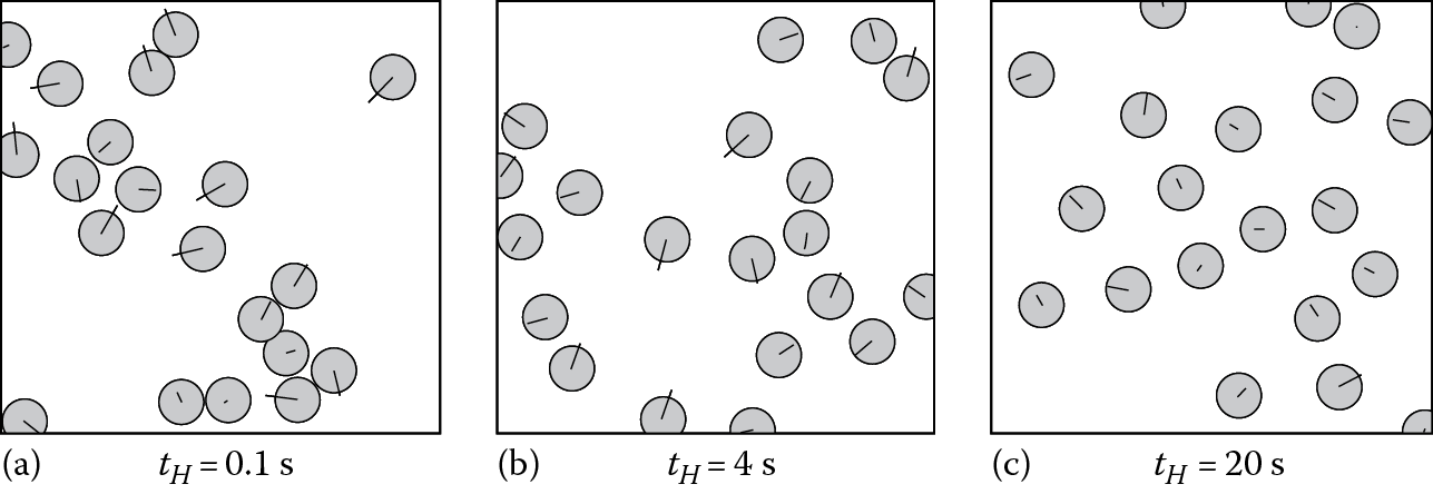
Effect of time horizon. Changing the time horizon, has a strong affect on an agent’s behavior. (a) With a too small value of t H , agents come very close and sometimes collide. (b) A moderate value of t H produces high-quality anticipatory motions. (c) If t H is too large, agents separate out in an unnatural way and may not reach their goals.
As mentioned before, the time horizon can be varied on a per-agent basis. Agents who are aggressive or impulsive can be given a smaller time horizon, and will perform many last minute avoidance maneuvers. Agents who are shy or tense can be given a larger time horizon and will react far in advance of any potential encounters.
19.4 Advanced Approaches
The collision-avoidance routine outlined earlier can provide robust, collision-free avoidance for many agents and works well in a wide variety of scenarios. However, recent work in crowd simulation and multiagent collision avoidance has gone beyond just modeling robust collision avoidance and focused on closely reproducing human behavior and providing rigorous guarantees on the quality of the motion.
19.4.1 Human Motion Simulation
Many assumptions we made in deriving the previous algorithm are unrealistic for modeling real humans. Our proposed model, for example, assumes that agents can see forever, know perfectly the radii and velocities of all of their neighbors, and are willing to come indefinitely close to any neighbors. Recent work such as the predictive avoidance method (PAM) provides some guidelines to making a more realistic model [Karamouzas 09].
19.4.1.1 Personal Space
Each agent in PAM has an additional safety distance that prefers to maintain from other agents in order to feel comfortable. This distance, along with the radius of the agent, defines the agent’s personal space. When computing the time to collision to each of its nearest neighbors, an agent in PAM tests for intersections between its personal space and the radius of its neighbor. This creates a small buffer between agents when they pass each other.
19.4.1.2 Field of View
Agents in PAM are not allowed to react to all the other agents in the environment, but rather are given a limited field of view in which they can sense. Often, the exact orientation of an agent is unknown, but we can generally use the (filtered) current velocity as an estimate of an agent’s facing direction. PAM agents use a field of view of ±100°, corresponding to the angle of sight of a typical human, and discard any agents who fall outside of this angle.
19.4.1.3 Distance to Collision
In PAM, agents reason about how far away (in meters) the point of collision is—defining a distance-to-collision, rather than a time-to-collision, formulation. This distance to collision is used to control the magnitude of the avoidance force. If the predicted collision point between two agents is closer than is allowed by an agent’s personal space the magnitude of the avoidance force rises steeply to help create an “impenetrable barrier” between agents. If the distance is further away than some maximum distance the avoidance force will be zero. Between and the magnitude is shaped to reduce jerky behavior.
19.4.1.3 Randomized Perturbation
In PAM, some perturbation is introduced in the collision-avoidance routine to account for the uncertainty that an agent has in sensing the velocities and radii of its nearby neighbors. Such perturbation is also needed to introduce irregularity among the agents and resolve artifacts that arise from perfectly symmetrical patterns (e.g., two agents on antipodal positions having exactly opposite directions). This perturbation can be expressed as a force that is added to the goal and collision-avoidance forces.
Figure 19.4 provides an illustration of the concept of an agent’s personal space and limited field of view. Figure 19.4 shows how the magnitude of the avoidance force falls off as a function of distance to collision. Finally, a simulation of two PAM agents was used to create the anticipatory avoidance example shown in Figure 19.1.
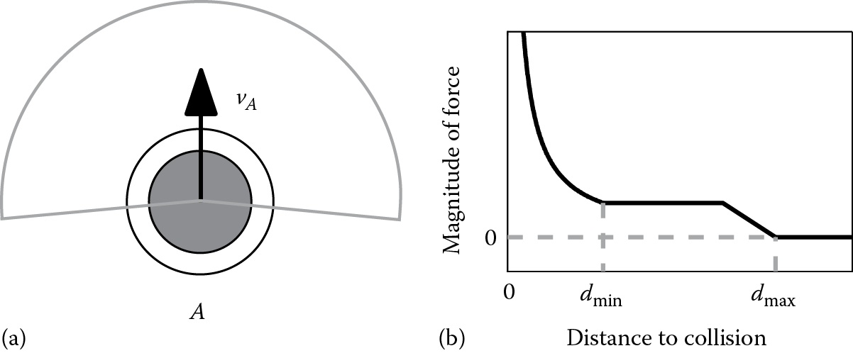
PAM agents’ parameters. (a) Here, agents have a limited field of view and an extended soft personal space past their radius (dashed circle). (b) The magnitude of the avoidance force is a function of the distance to collision that rises sharply when this distance is less than (the radius of the personal space) and falls to zero at some user-defined distance threshold
19.4.2 Guaranteed Collision Avoidance
Rather than trying to closely mimic the limitations of human sensing and planning, some researchers have focused on providing mathematically robust, guaranteed collision-free motion between multiple agents. The optimal reciprocal collision avoidance (ORCA) algorithm is one such approach, which is focused on decentralized, anticipatory collision avoidance between many agents [van den Berg 11].
The ORCA method works by defining a set of formal constraints on an agent’s velocity. When all agents follow these constraints, the resulting motion is provably collision-free, even with no communication between agents. In games, this formal guarantee of collision avoidance can be important, because it allows a high degree of confidence that the method will work well in challenging scenarios with fast-moving characters, quick dynamic obstacles, and very high density situations that can cause issues for many other avoidance methods.
Unlike PAM and the time-to-collision-based approach, which both use forces to steer an agent, ORCA is a velocity-based approach directly choosing a new velocity for each agent, at each time step. The idea of a velocity space can help illustrate how ORCA works. Unlike normal world space (Figure 19.5) where each 2D point represents a position, in velocity space, each 2D point represents an agent’s (relative) velocity. So the origin in velocity space, for example, represents an agent moving at the same speed as its neighbor. We can now designate the set of all velocities that lead to a collision before a given time horizon as forbidden and prevent agents from choosing those velocities for the next time step. This set of forbidden velocities is commonly called a velocity obstacle (VO). Figure 19.5 illustrates an agent’s velocity space and shades as gray the velocities that are forbidden. Because these forbidden velocities are based on future collisions, ORCA is a fundamentally anticipatory technique.
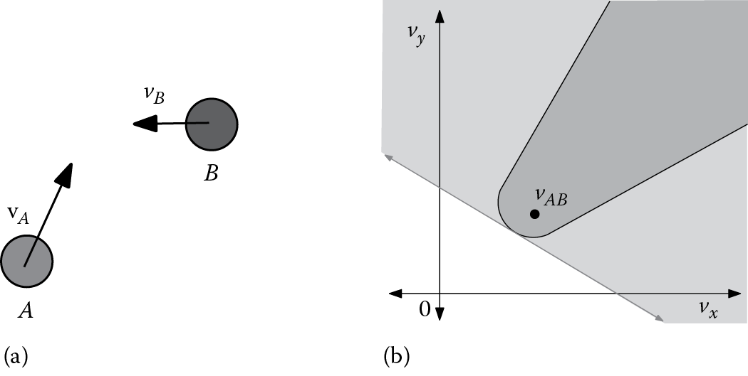
ORCA collision avoidance. (a) The world space shows the true position and velocities of two agents on a collision course. (b) Agent A ’s velocity space. The dark-shaded region shows the RVO (forbidden relative velocities), and the gray line shows a linear approximation of this space used by ORCA resulting in a larger forbidden region (both the light- and dark-shaded regions).
Conceptually, ORCA can be thought of as each agent on each time step, computing the VO for each of its neighbors and choosing a velocity outside the union of all VOs that is closest to its goal velocity. Unfortunately, directly implementing such an approach does not lead to great results. In practice, ORCA presents two important improvements to this simple approach in order to get efficient, stable motion. These changes derive from the key concepts of reciprocity and linearization.
In this context, reciprocity means the sharing of the collision-avoidance responsibility between two agents. Imagine Agents A and B on a collision course (as in Figure 19.5). If A chooses a velocity outside of the VO, that means it has resolved the collision completely on its own and B does not need to respond anymore. Likewise, if B avoids the entire collision, A should do nothing. Both agents choosing velocities outside the VOs will overly avoid the collision resulting in inefficient motion and can ultimately lead to distracting oscillations in an agent’s velocity. ORCA resolves this issue through the use of reciprocity, allowing each agent to avoid only part of the collision with the knowledge that the neighboring agent will resolve the reminder of the collision (a simple solution is to split the work 50–50 between the two agents). This modified set of forbidden velocities, which only avoid half of the collision, is known as a reciprocal velocity obstacle (RVO), which is illustrated as the dark-shaded region in Figure 19.5.
When there are multiple neighbors to avoid, each neighbor will cast a separate RVO onto the agent’s velocity. The agent should choose a new velocity outside the union of all these RVOs that is as close as possible to its goal velocity. Unfortunately, this is a complex, nonconvex space making it difficult to find an optimal noncolliding velocity. Potential approaches include randomly sampling velocities (as is implemented in the original RVO library) or testing all possible critical points that may be optimal (as implemented in ClearPath and HRVO [Gamma 14]). In contrast, ORCA avoids this issue by approximating each RVO with a single line. This linear approximation is called an ORCA constraint and is illustrated as the gray line in Figure 19.5. The result is an overapproximation with many new velocities now considered forbidden (i.e., both the dark- and the light-gray regions in Figure 19.5). However, the linearization is chosen to minimize approximation error near the current velocity, allowing ORCA to work well in practice. Because the union of a set of line constraints is convex, using only linear constraints greatly simplifies the optimization computation resulting in an order of magnitude speedup and allows some important guarantees of collision-freeness to be formally proved [van den Berg 11].
In some cases, the ORCA constraints may overconstrain an agent’s velocity leaving no valid velocity choice for this time step. In these cases, one option is to drop constraints from far away agents until a solution can be found. When constraints are dropped in this manner, the resulting motion is no longer guaranteed to be collision-free for that agent, for that time step. However, in practice, this typically results in only minor, fleeting collisions.
A complete C++ implementation of the ORCA algorithm is available online as part of the RVO2 collision-avoidance library (http://gamma.cs.unc.edu/RVO2/). This implementation is highly optimized, using a geometric approach to quickly compute both the RVOs and the ORCA constraints for every agent. The library then uses a randomized linear programming approach to efficiently find a velocity near the goal velocity that satisfies all the ORCA constraints. Using this optimized approach, ORCA can update agents’ states nearly as quickly as force-based methods, while still providing avoidance guarantees.
19.4.3 Herd’Em!
ORCA, and methods using similar geometric principles, has been integrated into many different computer games, both free and commercial. One freely available game that makes use of the library is Herd’Em! (http://gamma.cs.unc.edu/HERDEM/) [Curtis 10]. Herd’Em! simulates a flock of sheep and allows the user to control a sheepdog in an attempt to herd the sheep into the pen on the left side of the screen (Figure 19.6). The game uses a simple boids-like approach with one force pulling agents toward each other, one force encouraging some separation, and another force aligning the agents toward the same velocity. The new velocity as a result of these three forces is used to provide a goal velocity to ORCA. The ORCA simulation is set with a small time horizon, so that the flocking behavior is only modified when a collision is very imminent. This allows agents to flock nicely, while still guaranteeing collision avoidance.
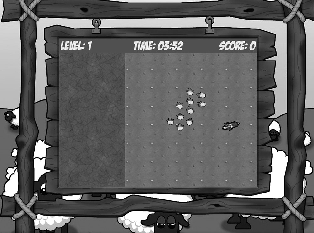
ORCA in practice. The game Herd’Em! combines a simple flocking method with ORCA to provide guaranteed collision avoidance of the characters under a wide variety of user inputs. (Courtesy of Dinesh Manocha, © 2012 University of North Carolina, Wilmington, NC. Used with permission.)
The guaranteed avoidance behavior is very important once a user is added in the loop. In Herd’Em!, every sheep feels an additional repulsive force away from the direction of the dog. As the user controls the dog by dragging it quickly around the screen, the dog can have a very high velocity. It is also common for users to try to stress the system by steering as many sheep as possible into a small corner. In both cases, the guaranteed avoidance of ORCA allows the simulation to remain collision-free despite the challenging conditions.
19.5 Conclusion
While anticipation in an agent’s motion is a wide-ranging topic, this chapter has covered many of the most important concepts to get started understanding the many exciting new developments in this area. Agent-based modeling, force-based versus velocity-space computations, time-to-collision calculations, time horizons, and goal velocities are all concepts that are central to a wide variety of character planning and navigation topics. While the code in Listing 19.3 provides good collision-avoidance behaviors in many situations, there is still room for improvement and exploration.
One exciting area of recent interest has been applying anticipatory collision-avoidance techniques to robots [Hennes 12]. An important consideration here is to robustly account for the uncertainty caused by imperfect sensing and actuation. Other interesting challenges include incorporating an agent’s anticipation into its character animation or adapting techniques such as ORCA to account for stress, cooperation, and other social factors. We hope the concepts and algorithm we have detailed in this chapter provide readers with a solid starting point for their own experimentations.
References
[Curtis 10] Curtis, S., Guy, S. J., Krajcevski, P., Snape, J., and D. Manocha. 2010. HerdEm. University of North Carolina, Wilmington, NC. http://gamma.cs.unc.edu/HERDEM/. (accessed January 10, 2015).
[Gamma 14] Manocha, D., Lin, M. et al. 2014. UNC GAMMA group’s collision avoidance libraries, University of North Carolina, Wilmington, NC. http://gamma.cs.unc.edu/CA/and http://gamma.cs.unc.edu/HRVO (accessed September 10, 2014).
[Guy 15] Guy S. J. and Karamouzas, I. 2015. Python implementation of the time-to-collision based force model. Game AI Pro Website. http://www.gameaipro.com (accessed February 7, 2015).
[Hennes 12] Hennes, D., Claes, D., Meeussen W., and K. Tuyls. 2012. Multi-robot collision avoidance with localization uncertainty. In Proceedings of the 11th International Conference on Autonomous Agents and Multiagent Systems, pp. 147–154.
[Karamouzas 09] Karamouzas, I., Heil, P., van Beek, P., and M. H. Overmars. 2009. A predictive collision avoidance model for pedestrian simulation. In Motion in Games, Lecture Notes in Computer Science 5884, eds. A. Egges, R. Geraerts, and M. Overmars, pp. 41–52. Springer-Verlag, Berlin, Germany.
[Snook 00] Snook, G. 2000. Simplified 3D movement and pathfinding using navigation meshes. In Game Programming Gems, ed. M. DeLoura, pp. 288–304. Charles River Media, Hingham, MA.
[Stout 00] Stout, B. 2000. The basics of A* for path planning. In Game Programming Gems, ed. M. DeLoura, pp. 254–263. Charles River Media, Hingham, MA.
[van den Berg 11] van den Berg, J., Guy, S. J., Lin, M., and D. Manocha. 2011. Reciprocal n-body collision avoidance. In Springer Tracts in Advanced Robotics, Vol. 70, eds. C. Pradalier, R. Siegwart, and G. Hirzinger, pp. 3–19. Springer-Verlag, Berlin, Germany.