
CHAPTER 5
SEMIRING VALUATION ALGEBRAS
The mathematical framework of valuation algebras introduced in Chapter 1 provides sufficient structure for the application of generic local computation methods. In the process, the numerous advantages of such a general framework became clear, and we have seen for ourselves that different formalisms are unified under this common perspective. As a fundamental requirement for this generality, we did not assume any further knowledge about the structure of valuations. They have only been considered as mathematical objects that possess a domain and that can further be combined and projected according to certain axioms. For certain applications, however, it is useful to have additional knowledge about the structure of valuations. This amounts to the identification of families of valuation algebra instances which share some common structure. A first example of such a family of valuation algebras grows out of the obvious similar structure of indicator functions and arithmetic potentials introduced as Instances 1.1 and 1.3. On the one hand, both instances are obtained by assigning values to tuples out of a finite set of tuples, but on the other hand, they differ in their definitions of combination and projection. Yet, there is a common ground between them. We will learn in this chapter that both examples belong to a family of instances, called semiring valuation algebras. A commutative semiring is by itself a fundamental algebraic structure that comprises a set of values and two operations called addition and multiplication. Then, the values assigned to tuples are those of the semiring, and the operations of combination and projection can both be expressed using the two semiring operations. In other words, every commutative semiring induces a new valuation algebra, and the two examples of indicator functions and arithmetic potentials are both members of this large family. The reasons why we are interested in semiring valuation algebras are manifold. First and foremost, semiring instances are very large in number and, because each commutative semiring gives rise to a valuation algebra, we naturally obtain as many new valuation algebras as commutative semirings exist. Moreover, if we interpret valuation algebras as formalisms for knowledge representation, we are not even able to explain for some of these instances what kind of knowledge they model. Nevertheless, we have efficient algorithms for their processing thanks to the local computation framework. Second, we will see that a single verification proof of the valuation algebra axioms covers all formalisms that adopt this common structure, and we are also relieved from searching each formalism separately for neutral elements, null elements and the presence of a division operator. Finally, semiring valuations also stimulate new applications of local computation techniques that go beyond the pure computation of inference. Solution construction in constraint systems is an example of such an application that will be discussed in Chapter 8. Besides semiring valuation algebras, there are other families of formalisms derived in a similar way from other algebraic structures. This powerful technique is called generic construction and takes center stage in the second part of this book.
This chapter starts with a general introduction to semiring theory, accompanied by a large catalogue of instances to convince the reader of the richness of semiring examples. Section 5.2 then studies different classes of semirings that arise from the properties of a canonical order relation. Following (Kohlas & Wilson, 2008), we then show in Section 5.3 how semirings produce valuation algebras and we give an extensive member list of this family of valuation algebras in Section 5.4. Section 5.5 deals with the algebraic properties of semiring valuations and show which properties of the semiring guarantee the existence of neutral and null elements. The study of division is again postponed to the chapter appendix. A second family of valuation algebras, which is closely related to semiring valuations, is introduced in Section 5.7, and its algebraic properties are analyzed in Section 5.8.
5.1 SEMIRINGS
A semiring is an algebraic structure consisting of a set provided with two operations, called addition and multiplication, which satisfy the distributive law. In recent years, the importance of semirings for computational purposes has grown significantly and the distributive law is in fact the reason for this increasing popularity. From the simple formula a × (b + c) = a × b + a × c, we can directly observe that the left-hand side is computationally more efficient since we perform only one multiplication. The distributive law is the cause of efficiency of local computation, since it induces the combination axiom. However, let us start with a short introduction to semiring theory.
Definition 5.1 A tuple ![]() with binary operations + and × is called semiring if the following properties hold:
with binary operations + and × is called semiring if the following properties hold:
(S1) ![]()
(S2) ![]()
(S3) ![]()
(S4) ![]()
(S6) ![]()
(S7) ![]()
There are different definitions of semirings in the literature. This definition is taken from (Golan, 1999) and assumes the existence of two neutral elements. The neutral element 0 ![]() A with respect to addition is sometimes called zero element. It is a simple consequence of (S5) that a zero element is always unique. Moreover, if an algebraic structure provides all properties of a semiring except the presence of a zero element then the latter can always be adjoined artificially. The neutral element 1
A with respect to addition is sometimes called zero element. It is a simple consequence of (S5) that a zero element is always unique. Moreover, if an algebraic structure provides all properties of a semiring except the presence of a zero element then the latter can always be adjoined artificially. The neutral element 1 ![]() A with respect to multiplication is called unit element. It is also unique but in contrast to the zero element, it can only be adjoined if the operation of addition is idempotent (see Definition 5.2 below). The corresponding constructions are shown in (Kohlas & Wilson, 2008).
A with respect to multiplication is called unit element. It is also unique but in contrast to the zero element, it can only be adjoined if the operation of addition is idempotent (see Definition 5.2 below). The corresponding constructions are shown in (Kohlas & Wilson, 2008).
Definition 5.2 Let ![]() be a semiring:
be a semiring:
- it is called commutative if a × b = b × a for all a, b
 A;
A; - it is called idempotent if a + a = a for all a
 A;
A; - it is called positive if a + b = 0 implies that a = b = 0 for all a, b
 A;
A;
Let us consider some examples of semirings:
Example 5.1 (Arithmetic Semirings) Consider the set of non-negative real numbers ![]() ≤ with + and × designating the usual operations of addition and multiplication. This is clearly a positive, commutative semiring with the number 0 as zero element and the number 1 as unit element. In the same way, we could also take the fields of complex, real or rational numbers, or alternatively only non-negative integers or non-negative rationals. In the former three cases, the semiring would not be positive anymore, whereas ordinary addition and multiplication on non-negative integers and rationals yield again a positive semiring.
≤ with + and × designating the usual operations of addition and multiplication. This is clearly a positive, commutative semiring with the number 0 as zero element and the number 1 as unit element. In the same way, we could also take the fields of complex, real or rational numbers, or alternatively only non-negative integers or non-negative rationals. In the former three cases, the semiring would not be positive anymore, whereas ordinary addition and multiplication on non-negative integers and rationals yield again a positive semiring.
Example 5.2 (Boolean Semiring) Take the set ![]() = {0,1} with the intention that 0 designates the truth value “false” and 1 “true”. Addition is defined as a + b = max{a, b} and represents the logical disjunction. Similarly, multiplication is defined as a × b = min{a, b} which stands for the logical conjunction. This is a commutative, positive and idempotent semiring with zero element 0 and unit element 1.
= {0,1} with the intention that 0 designates the truth value “false” and 1 “true”. Addition is defined as a + b = max{a, b} and represents the logical disjunction. Similarly, multiplication is defined as a × b = min{a, b} which stands for the logical conjunction. This is a commutative, positive and idempotent semiring with zero element 0 and unit element 1.
Example 5.3 (Bottleneck Semiring) A generalization of the Boolean semiring is obtained if we take a + b = max{a, b} and a × b = min{a, b} over the set of real numbers ![]() . Then,
. Then, ![]() is the zero element,
is the zero element, ![]() the unity, and the semiring remains commutative, positive and idempotent.
the unity, and the semiring remains commutative, positive and idempotent.
Example 5.4 (Tropical Semiring) An important semiring is defined over the set of non-negative integers ![]() with a + b = min{a, b} and the usual integer addition +
with a + b = min{a, b} and the usual integer addition +![]() for × with the convention that a
for × with the convention that a ![]() . This semiring is commutative, positive and idempotent,
. This semiring is commutative, positive and idempotent, ![]() is the zero element and the integer 0 is the unit element.
is the zero element and the integer 0 is the unit element.
Example 5.5 (Arctic Semiring) The arctic semiring takes max for addition over the set of real numbers ![]() . Multiplication is +
. Multiplication is +![]() with a
with a ![]() . This semiring is commutative, positive and idempotent, has
. This semiring is commutative, positive and idempotent, has ![]() as zero element and 0 as unit element.
as zero element and 0 as unit element.
Example 5.6 (Truncation Semiring) An interesting variation of the tropical semiring is obtained if we take A = {0, …, k} for some integer k. Addition corresponds again to minimization but this time, we take the truncated integer addition for x, i.e. a × b = min{a +![]() b, k}. This is a commutative, positive and idempotent semiring with k being the zero element and 0 the unit.
b, k}. This is a commutative, positive and idempotent semiring with k being the zero element and 0 the unit.
Example 5.7 (Semiring of Formal Languages) A string is a finite sequence of symbols from a countable alphabet ∑ and a set of strings is called language. In particular, we refer to the language of all possible strings over the alphabet ∑ as ∑*. For A, B ![]() we define A + B = A ∪ B and A × B = {ab |a
we define A + B = A ∪ B and A × B = {ab |a ![]() A and b
A and b ![]() B}. This semiring of formal languages is idempotent with zero element
B}. This semiring of formal languages is idempotent with zero element ![]() and unit element
and unit element ![]() . It is also positive but not commutative.
. It is also positive but not commutative.
Example 5.8 (Triangular Norm Semiring) Triangular norms (t-norms) were originally introduced in the context of probabilistic metric spaces (Menger, 1942; Schweizer & Sklar, 1960). They represent binary operations on the unit interval [0,1] which are commutative, associative, nondecreasing in both arguments, and have the number 1 as unit and 0 as zero element:
1. ![]() we have T(a, b) = T(b, a) and T(a, T(b, c)) = T(T(a, b), c),
we have T(a, b) = T(b, a) and T(a, T(b, c)) = T(T(a, b), c),
2. a ≤ a’ and b ≤ b’ imply T(a, b) ≤ T(a’, b’),
3. ![]() we have T(a, 1) = T(1, a) = a and T(a, 0) = T(0, a) = 0.
we have T(a, 1) = T(1, a) = a and T(a, 0) = T(0, a) = 0.
T-norms are used in fuzzy set theory and possibility theory. In order to obtain a semiring, we define the operation × on the unit interval by a t-norm and + as max. This is a commutative, positive and idempotent semiring with the number 0 as zero element and 1 as unit. Here are some typical t-norms:
- Minimum T-Norm: T(a, b) = min{a, b}.
- Product T-Norm: T(a, b) = a · b.
- Lukasiewicz T-Norm: T(a, b) = max{a + b - 1, 0}.
- Drastic Product: T(a, 1) = T(1, a) = a and T(a, b) = 0 in all other cases.
The semiring induced by the product t-norm is also called probabilistic semiring. Instead of maximization, we may also take minimization for addition, which only reverses the definition of zero and unit element.
In addition to these examples, we may also define structures to derive semirings from other semirings. Vectors and matrices with semiring values are typical examples that form themselves a semiring.
5.1.1 Multidimensional Semirings
Take n possibly different semirings ![]() for i = 1, …, n and define
for i = 1, …, n and define
![]()
with corresponding, component-wise operations
![]()
These operations inherit associativity, commutativity and distributivity from their components. Hence, ![]() becomes itself a semiring with zero element 0 = (01, …, 0n) and unit 1 = (1i, …, 1n). If all Ai are commutative, positive or idempotent, then so is A.
becomes itself a semiring with zero element 0 = (01, …, 0n) and unit 1 = (1i, …, 1n). If all Ai are commutative, positive or idempotent, then so is A.
5.1.2 Semiring Matrices
Given a semiring ![]() and n
and n ![]() , we consider the set
, we consider the set ![]() of n × n matrices with elements in A. Addition and multiplication of semiring matrices is defined in the usual way:
of n × n matrices with elements in A. Addition and multiplication of semiring matrices is defined in the usual way:
(5.1) ![]()
and
(5.2) ![]()
for 1 ≤ i, j ≤ n. It is easy to see that square matrices over a semiring themselves form a semiring. Also, we obtain the zero element for semiring matrices by O(i,j) = 0 for 1 ≤ i, j ≤ n and likewise, we obtain the unit element for the algebra of semiring matrices by I(i, j) = 1 if i = j and I(i, j) = 0 otherwise. Finally, if ![]() is positive or idempotent, then so are matrices over this semiring, but this does not hold for commutativity. Note in particular that ordinary real-valued, square matrices of the same order form a semiring.
is positive or idempotent, then so are matrices over this semiring, but this does not hold for commutativity. Note in particular that ordinary real-valued, square matrices of the same order form a semiring.
5.2 SEMIRINGS AND ORDER
The substructure ![]() is a commutative monoid with neutral element, which makes it always possible (Gondran & Minoux, 2008) to introduce a canonical preorder (see Definition A.2 in the appendix of Chapter 1). We define for a, b
is a commutative monoid with neutral element, which makes it always possible (Gondran & Minoux, 2008) to introduce a canonical preorder (see Definition A.2 in the appendix of Chapter 1). We define for a, b ![]() A:
A:
Lemma 5.1 The Relation (5.3) is a preorder, i.e. reflexive and transitive.
Proof: Reflexivity follows from the existence of a neutral element. Since a + 0 = a we have a ≤ a for all a ![]() A. To prove transitivity, let us assume that a ≤ b and b ≤ d. Consequently, there exist c, c’
A. To prove transitivity, let us assume that a ≤ b and b ≤ d. Consequently, there exist c, c’ ![]() A such that a + c = b and b + c’ = d. We have a + c + c’ = d and therefore a ≤ d.
A such that a + c = b and b + c’ = d. We have a + c + c’ = d and therefore a ≤ d. ![]()
The following lemma ensures that the canonical preorder is compatible with both semiring operations.
Lemma 5.2 The canonical preorder of a semiring ![]() satisfies:
satisfies:
Proof:
1. Assume a ≤ b, i.e. there exists x ![]() A such that a + x = b. Then, (a + c) + x = b + c and therefore a + c ≤ b + c.
A such that a + x = b. Then, (a + c) + x = b + c and therefore a + c ≤ b + c.
2. Assume a ≤ b, i.e. there exists x ![]() A such that a + x = b. Then (a + x) × c = (a × c) + (x × c) = b × c and therefore a × c ≤ b × c. The proof of the second statement is symmetric.
A such that a + x = b. Then (a + x) × c = (a × c) + (x × c) = b × c and therefore a × c ≤ b × c. The proof of the second statement is symmetric.
3. Since 0 + b = b we clearly have 0 ≤ b. Using Property (SP1) we further derive a + 0 ≤ a + b. Hence, a ≤ a + b and a similar argument shows b ≤ a + b.
The canonical preorder of a semiring is in general not antisymmetric. Take for example the arithmetic semiring of integers ![]() and observe that
and observe that ![]() . This is a consequence of the existence of additive inverses. Antisymmetry is therefore compatible with the existence of additive inverses or, in other words, with the ring structure of
. This is a consequence of the existence of additive inverses. Antisymmetry is therefore compatible with the existence of additive inverses or, in other words, with the ring structure of ![]() . This is also indicated by Property (SP3) of the above lemma. However, if the canonical preorder is antisymmetric, it is called a partial order (see Definition A.2 in the appendix of Chapter 1) and the semiring becomes a dioid (Gondran & Minoux, 2008). A sufficient condition is idempotency.
. This is also indicated by Property (SP3) of the above lemma. However, if the canonical preorder is antisymmetric, it is called a partial order (see Definition A.2 in the appendix of Chapter 1) and the semiring becomes a dioid (Gondran & Minoux, 2008). A sufficient condition is idempotency.
Lemma 5.3 If ![]() is an idempotent semiring, we may characterize the canonical preorder (5.3) as
is an idempotent semiring, we may characterize the canonical preorder (5.3) as
Proof: It is sufficient to show that a ≤ b according to (5.3) implies a + b = b. Suppose a ≤ b, i.e. there exists c ![]() A such that a + c = b. We then have by idempotency a + b = a + a + c = a + c = b.
A such that a + c = b. We then have by idempotency a + b = a + a + c = a + c = b. ![]()
Lemma 5.4 The Relation (5.4) is a partial order.
Proof: Since the two relations (5.3) and (5.4) are equivalent in case of an idem-potent semiring, we obtain reflexivity and transitivity from Lemma 5.1. To prove antisymmetry, we assume that a ≤ b and b ≤ a, i.e. a + b = b and b + a = a. Consequently, a = a + b = b and therefore a = b. ![]()
An idempotent semiring is therefore always a dioid and we refer to Relation (5.4) as its canonical partial order.
Example 5.9 We already pointed out that the canonical preorder in the arithmetic semiring ![]() is not antisymmetric and therefore not a partial order. Restricting this semiring to non-negative integers
is not antisymmetric and therefore not a partial order. Restricting this semiring to non-negative integers ![]() turns the canonical preorder into a partial order. This is an example of a dioid that is not idempotent and shows that idempotency is indeed only a sufficient condition for a canonical partial order. The examples 5.2 to 5.8 are all idempotent and thus dioids. However, it is important to remark that the canonical semiring order does not necessarily agree with the natural order between number. Take for example the tropical semiring
turns the canonical preorder into a partial order. This is an example of a dioid that is not idempotent and shows that idempotency is indeed only a sufficient condition for a canonical partial order. The examples 5.2 to 5.8 are all idempotent and thus dioids. However, it is important to remark that the canonical semiring order does not necessarily agree with the natural order between number. Take for example the tropical semiring ![]() where the relation (5.4) becomes a ≤ b if and only if, min{a, b} = b. Here, the canonical semiring order corresponds to the inverse of the natural order between natural numbers.
where the relation (5.4) becomes a ≤ b if and only if, min{a, b} = b. Here, the canonical semiring order corresponds to the inverse of the natural order between natural numbers.
Two further properties of idempotent semirings are listed in the following lemma. In particular, we learn from (SP5) why all idempotent semirings in the example catalogue of Section 5.1 are positive.
Lemma 5.5 Let ![]() be an idempotent semiring.
be an idempotent semiring.
Proof:
1. According to Property (SP3) a, b ≤ a + b. Let c ![]() A be another upper bound for a and b, i.e. a ≤ c and b ≤ c. We conclude from a + c = c and b + c = c that (a + c) + (b + c) = c + c and by idempotency (a + b) + c = c. Consequently, a + b ≤ c which implies that a + b is the least upper bound of a and b.
A be another upper bound for a and b, i.e. a ≤ c and b ≤ c. We conclude from a + c = c and b + c = c that (a + c) + (b + c) = c + c and by idempotency (a + b) + c = c. Consequently, a + b ≤ c which implies that a + b is the least upper bound of a and b.
2. Suppose that a + b = 0. Applying Property (SP3) we obtain 0 ≤ a ≤ a + b = 0 and by transitivity and antisymmetry we conclude that a = 0. Similarly, we prove b = 0.
Definition 5.3 If a semiring ![]() satisfies a + 1 = 1 for all a
satisfies a + 1 = 1 for all a ![]() A, then it is called bounded semiring. If also commutativity holds, the semiring is called c-semiring (constraint semiring).
A, then it is called bounded semiring. If also commutativity holds, the semiring is called c-semiring (constraint semiring).
This definition comes from (Mohri, 2002; Bistarelli et al., 2002) and characterizes bounded semirings by the fact that the unit element is absorbing with respect to addition. Also, bounded semirings are close to simple semirings in (Lehmann, 1976). We first remark that bounded semirings are idempotent, since 1 + 1 = 1 implies that a + a = a for all a ![]() A. This follows from distributivity: a + a = 1 × (a + a) = (1 × a) + (1 × a) = (1 + 1) × a = 1 × a = a. Consequently, the relation ≤ is a partial order which furthermore satisfies the following properties.
A. This follows from distributivity: a + a = 1 × (a + a) = (1 × a) + (1 × a) = (1 + 1) × a = 1 × a = a. Consequently, the relation ≤ is a partial order which furthermore satisfies the following properties.
Lemma 5.6 Let ![]() be a bounded semiring.
be a bounded semiring.
Proof:
1. From Definition 5.3 follows that a ≤ 1 for all a ![]() A. Because Property (SP3) still holds, it remains to be proved that a × b ≤ a for all a, b
A. Because Property (SP3) still holds, it remains to be proved that a × b ≤ a for all a, b ![]() A. This claim results from the distributive law since a + (a × b) = (a × 1) + (a × b) = a × (1 + b) = a × 1 = a.
A. This claim results from the distributive law since a + (a × b) = (a × 1) + (a × b) = a × (1 + b) = a × 1 = a.
2. By Property (SP6) we have a × b ≤ a, b. Let c be another lower bound of a and b, i.e. c ≤ a and c ≤ b. Then, by (SP2) c × b ≤ a × b. Similarly, we derive from c ≤ b that c = c × c ≤ c × b and therefore by transitivity c ≤ a × b. Thus, a × b is the greatest lower bound. ![]()
With supremum and infimum according to (SP4) and (SP7), c-semirings with idempotent multiplication adopt the structure of a lattice according to Definition A.5 in the appendix of Chapter 1. Moreover, the following theorem states that it is even distributive. This has been remarked by (Bistarelli et al., 1997), but in contrast to this reference it is not necessarily complete since we do not assume infinite summation in the definition of a c-semiring.
Theorem 5.1 A c-semiring with idempotent multiplication is a bounded, distributive lattice with a ![]() b and
b and ![]() .
.
Proof: It remains to prove that the two operations + and × distribute over each other in the case of an idempotent c-semiring. By definition, × distributes over +. On the other hand, we have for a, b, c ![]() A
A
We therefore have a distributive lattice. Since a + 1 = 1 and a × 0 = 0 for all a ![]() A the lattice is bounded with bottom element 0 and top element 1.
A the lattice is bounded with bottom element 0 and top element 1.
Example 5.10 The Boolean semiring of Example 5.2, the bottleneck semiring of Example 5.3, the tropical semiring of Example 5.4, the truncation semiring of Example 5.6 and all t-norm semirings of Example 5.8 are c-semirings and therefore also bounded. Among them, multiplication is idempotent in the Boolean semiring and in the bottleneck semiring which therefore become bounded, distributive lattices. Note also that if all semirings are c-semirings, then so is the induced multidimensional semiring. A similar statement does not hold for the semiring of matrices.
Example 5.11 (Semiring of Boolean Functions) Consider a set of r ![]() propositional variables. Then, the set of all Boolean functions f:
propositional variables. Then, the set of all Boolean functions f: ![]() forms a semiring with addition f + g = max{f, g} and multiplication f × g = min{f, g}, both being evaluated point-wise. If f0 denotes the constant mapping to 0 and f1 the constant mapping to 1, then f0 is the zero element and f1 the unit element of the semiring. The semiring is a c-semiring and since multiplication is also idempotent, this semiring is a distributive lattice. In particular, the semiring of Boolean functions with r = 0 corresponds to the Boolean semiring of Example 5.2 where the two and only elements f0 and f1 are identified with their values 0 and 1.
forms a semiring with addition f + g = max{f, g} and multiplication f × g = min{f, g}, both being evaluated point-wise. If f0 denotes the constant mapping to 0 and f1 the constant mapping to 1, then f0 is the zero element and f1 the unit element of the semiring. The semiring is a c-semiring and since multiplication is also idempotent, this semiring is a distributive lattice. In particular, the semiring of Boolean functions with r = 0 corresponds to the Boolean semiring of Example 5.2 where the two and only elements f0 and f1 are identified with their values 0 and 1.
Conversely to Theorem 5.1, we note that every bounded, distributive lattice (see Definition A.6 in the appendix of Chapter 1) is an idempotent semiring with join for + and meet for x. The bottom element ![]() of the lattice becomes the zero element and the top element
of the lattice becomes the zero element and the top element ![]() becomes the unit element. Thus, this semiring is even a c-semiring with idempotent multiplication. We therefore have an equivalence between the two structures and conclude that the powerset lattice of Example A.2 and the division lattice of Example A.3 are both c-semirings with idempotent multiplication. There are naturally many other semiring examples that have not appeared in this chapter. For example, we mention that every (unit) ring is a semiring with the additional property that inverse additive elements exist. In the same breath, fields are rings with multiplicative inverses. These remarks lead to further semiring examples such as the ring of polynomials or the Galois field. We also refer to (Davey & Priestley, 1990) for a broad listing of further examples of distributive lattices and to the comprehensive literature about semirings (Golan, 1999; Golan, 2003; Gondran & Minoux, 2008).
becomes the unit element. Thus, this semiring is even a c-semiring with idempotent multiplication. We therefore have an equivalence between the two structures and conclude that the powerset lattice of Example A.2 and the division lattice of Example A.3 are both c-semirings with idempotent multiplication. There are naturally many other semiring examples that have not appeared in this chapter. For example, we mention that every (unit) ring is a semiring with the additional property that inverse additive elements exist. In the same breath, fields are rings with multiplicative inverses. These remarks lead to further semiring examples such as the ring of polynomials or the Galois field. We also refer to (Davey & Priestley, 1990) for a broad listing of further examples of distributive lattices and to the comprehensive literature about semirings (Golan, 1999; Golan, 2003; Gondran & Minoux, 2008).
5.3 SEMIRING VALUATION ALGEBRAS
Equipped with this catalogue of semiring examples, we will now come to the main part of this chapter and show how semirings induce valuation algebras by a mapping from tuples to semiring values. This theory was developed in (Kohlas, 2004; Kohlas & Wilson, 2006; Kohlas & Wilson, 2008), who also substantiated for the first time the relationship between semiring properties and the attributes of their induced valuation algebras. In particular, we will discover that formalisms for constraint modelling are an important subgroup of semiring valuation algebras. For this reason, we subsequently prefer the term configuration instead of tuple which is more common in constraint literature. In this context, a similar framework to abstract constraint satisfaction problems was introduced by (Bistarelli et al., 1997; Bistarelli et al., 2002). The importance of such formalisms outside the field of constraint satisfaction was furthermore explored by (Aji, 1999; Aji & McEliece, 2000), who also proved the applicability of the Shenoy-Shafer architecture. However, this is only one of many conclusions to which we come by showing that semiring-based formalisms satisfy the valuation algebra axioms.
To start with, consider a commutative semiring ![]() and a set r of variables with finite frames. A semiring valuation
and a set r of variables with finite frames. A semiring valuation ![]() with domain s
with domain s ![]() r is defined to be a function that associates a value from A with each configuration
r is defined to be a function that associates a value from A with each configuration ![]() ,
,
![]()
Remember that ![]() such that a semiring valuation on the empty domain is
such that a semiring valuation on the empty domain is ![]() . We subsequently denote the set of all semiring valuations with domain s by
. We subsequently denote the set of all semiring valuations with domain s by ![]() and use Φ for all semiring valuations whose domains belong to the powerset lattice D = P(r). Next, the following operations in
and use Φ for all semiring valuations whose domains belong to the powerset lattice D = P(r). Next, the following operations in ![]() are introduced:
are introduced:
Note that the definition of projection is well defined due to the associativity and commutativity of semiring addition and the finiteness of the domains. We now arrive at the central theorem of this chapter which states that we obtain a valuation algebra from every commutative semiring through the above generic construction:
Theorem 5.2 A system of semiring valuations ![]() with respect to a commutative semiring
with respect to a commutative semiring ![]() with labeling, combination and projection as defined above, satisfies the axioms of a valuation algebra.
with labeling, combination and projection as defined above, satisfies the axioms of a valuation algebra.
Proof: We verify the Axioms (A1) to (A6) of a valuation algebra given in Section 1.1. Observe that the labeling (A2), projection (A3) and domain (A6) properties are immediate consequences of the above definitions.
(A1) Commutative Semigroup: The commutativity of combination follows directly from the commutativity of the × operation in the semiring A and the definition of combination. To prove associativity, assume that ![]() , Ψ and
, Ψ and ![]() are valuations with domains
are valuations with domains ![]() , then for
, then for ![]()
The same result is obtained in exactly the same way for ![]() which proves associativity.
which proves associativity.
(A4) Transitivity: Transitivity of projection means simply that we can sum out variables in two steps. That is, if ![]() , then, for all
, then, for all ![]() .
.
(A5) Combination: Suppose that ![]() has domain t and Ψ domain u and
has domain t and Ψ domain u and ![]() , where
, where ![]() . Using the distributivity of semiring multiplication over addition, we obtain for
. Using the distributivity of semiring multiplication over addition, we obtain for ![]() ,
,
To sum it up, a simple mapping from configurations to the values of a commutative semiring provides sufficient structure to give rise to a valuation algebra. The listing of semirings given in the two foregoing sections served to exemplify the semiring concepts introduced beforehand. We are next going to reconsider these semirings in order to show which valuation algebras they concretely induce. We will meet familiar instances such as arithmetic potentials or indicator functions, but also many new instances that considerably extend the valuation algebra catalogue of Chapter 1.
5.4 EXAMPLES OF SEMIRING VALUATION ALGEBRAS
If we consider the arithmetic semiring ![]() of non-negative real numbers presented in Section 5.1, we come across the valuation algebra of arithmetic potentials introduced as Instance 1.3. It is easy to see that both operations defined for semiring valuations correspond exactly to the operations for arithmetic potentials in equation (1.10) and (1.11). Therefore, the proof of Theorem 5.2 also delivers the promised argument that arithmetic potentials indeed satisfy the valuation algebra axioms. Moreover, since the arithmetic semiring can be built on complex numbers, we also come to the conclusion that the formalism used for the discrete Fourier transform in Instance 2.6 forms a valuation algebra. Similar statements hold for the valuation algebras of indicator functions, Boolean functions, crisp constraints or the relational algebra that are induced by the Boolean semiring
of non-negative real numbers presented in Section 5.1, we come across the valuation algebra of arithmetic potentials introduced as Instance 1.3. It is easy to see that both operations defined for semiring valuations correspond exactly to the operations for arithmetic potentials in equation (1.10) and (1.11). Therefore, the proof of Theorem 5.2 also delivers the promised argument that arithmetic potentials indeed satisfy the valuation algebra axioms. Moreover, since the arithmetic semiring can be built on complex numbers, we also come to the conclusion that the formalism used for the discrete Fourier transform in Instance 2.6 forms a valuation algebra. Similar statements hold for the valuation algebras of indicator functions, Boolean functions, crisp constraints or the relational algebra that are induced by the Boolean semiring ![]() {0, 1}, max, min, 0, 1
{0, 1}, max, min, 0, 1![]() . Again, if we replace semiring addition and multiplication in equation (5.5) and (5.6) by the corresponding operations max and min, we obtain the combination and projection rules given in Instance 1.1.
. Again, if we replace semiring addition and multiplication in equation (5.5) and (5.6) by the corresponding operations max and min, we obtain the combination and projection rules given in Instance 1.1.
![]() 5.1 Weighted Constraints - Spohn Potentials - GAI Preferences
5.1 Weighted Constraints - Spohn Potentials - GAI Preferences
Besides crisp constraints, alternative constraint systems may be derived by examining other semirings: the tropical semiring ![]() of Example 5.4 induces the valuation algebra of weighted constraints (Bistarelli et al., 1997; Bistarelli et al., 1999). This formalism also corresponds to Spohn potentials (Spohn, 1988) which have been proposed as a dynamic theory of graded belief states based on ordinary numbers. (Kohlas, 2003) delivers the explicit proof that weighted constraints satisfy the valuation algebra axioms. But in our context of semiring valuation algebras, this insight follows naturally from Theorem 5.2. No further proof is necessary. We again refer to later sections for concrete applications based on weighted constraints that in turn give birth to further inference problems. Here, we content ourselves with a small example on how to compute with weighted constraints.
of Example 5.4 induces the valuation algebra of weighted constraints (Bistarelli et al., 1997; Bistarelli et al., 1999). This formalism also corresponds to Spohn potentials (Spohn, 1988) which have been proposed as a dynamic theory of graded belief states based on ordinary numbers. (Kohlas, 2003) delivers the explicit proof that weighted constraints satisfy the valuation algebra axioms. But in our context of semiring valuation algebras, this insight follows naturally from Theorem 5.2. No further proof is necessary. We again refer to later sections for concrete applications based on weighted constraints that in turn give birth to further inference problems. Here, we content ourselves with a small example on how to compute with weighted constraints.
Let r = {A, B, C} be a set of three variables with finite frames ![]() and
and ![]() . We define two weighted constraints c1 and c2 with domain d(c1) = {A, B} and d(c2) = {B, C}:
. We define two weighted constraints c1 and c2 with domain d(c1) = {A, B} and d(c2) = {B, C}:
We combine c1 and c2 and project the result to {A, C}
Alternatively to the tropical semiring, we may also take the arctic semiring ![]() of Example 5.5 to build weighted constraints, which then corresponds to the formalism of generalized additive independent preferences (GAI preferences) (Fishburn, 1974; Bacchus & Adam, 1995). The modification of the above example to weighted constraints induced by the arctic semiring is left to the reader.
of Example 5.5 to build weighted constraints, which then corresponds to the formalism of generalized additive independent preferences (GAI preferences) (Fishburn, 1974; Bacchus & Adam, 1995). The modification of the above example to weighted constraints induced by the arctic semiring is left to the reader.
![]() 5.2 Possibility Potentials - Probabilistic Constraints - Fuzzy Sets
5.2 Possibility Potentials - Probabilistic Constraints - Fuzzy Sets
The very popular valuation algebra of possibility potentials is induced by the triangular norm semirings ![]() [0, 1], max, t-norm, 0, 1
[0, 1], max, t-norm, 0, 1![]() of Example 5.8. Historically, possibility theory was proposed by (Zadeh, 1978) as an alternative approach to probability theory, and (Shenoy, 1992a) furnished the explicit proof that this formalism indeed satisfies the valuation algebra axioms. This was limited to some specific t-norms and (Kohlas, 2003) generalized the proof to arbitrary t-norms. However, thanks to the generic construction of semiring valuations, the general statement that possibility potentials form a valuation algebra under any t-norm follows immediately from Theorem 5.2. We also refer to (Schiex, 1992) which unified this and the foregoing instance to possibilistic constraints.
of Example 5.8. Historically, possibility theory was proposed by (Zadeh, 1978) as an alternative approach to probability theory, and (Shenoy, 1992a) furnished the explicit proof that this formalism indeed satisfies the valuation algebra axioms. This was limited to some specific t-norms and (Kohlas, 2003) generalized the proof to arbitrary t-norms. However, thanks to the generic construction of semiring valuations, the general statement that possibility potentials form a valuation algebra under any t-norm follows immediately from Theorem 5.2. We also refer to (Schiex, 1992) which unified this and the foregoing instance to possibilistic constraints.
To give an example of how to compute with possibility potentials, we settle for the use of the Lukasiewicz t-norm defined as a × b = max{a + b - 1, 0} for all ![]() [0, 1]. Again, let r = {A, B, C} be a set of three variables with finite frames
[0, 1]. Again, let r = {A, B, C} be a set of three variables with finite frames ![]() and
and ![]() . We define two possibility
. We define two possibility
potentials p1 and p2 with domain d(p1) = {A, B} and d(p2) = {B, C}:
We combine p1 and p2 and project the result to {A, C}

Particularly important among these t-norms is ordinary multiplication. The valuation algebra induced by the corresponding probabilistic semiring of Example 5.8 is known as the formalism of probabilistic constraints (Bistarelli & Rossi, 2008) or fuzzy subsets (Zadeh, 1978). An example can easily be obtained from the arithmetic potentials presented as Instance 1.3. Combination is identical for both instances such that only projection, which now consists of maximization instead of summation, has to be recomputed.
![]() 5.3 Set-based Constraints - Assumption-based Constraints
5.3 Set-based Constraints - Assumption-based Constraints
The valuation algebra induced by the powerset lattice of Example A.2 in the appendix of Chapter 1 corresponds to the formalism of set-based constraints (Bistarelli et al., 1997). Imagine two prepositional variables A1 and A2. We then build the powerset lattice from their configuration set P({(0, 0), …, (1, 1)}) and obtain a complete, distributive lattice according to Example A.2. To introduce valuations that assign values from this semiring, let r = {A, B, C} be a set of three variables with finite frames ![]() and
and ![]() . We define two set-based constraint c1 and c2 with domain d(c1) = {A, B} and d(c2) = {B, C}:
. We define two set-based constraint c1 and c2 with domain d(c1) = {A, B} and d(c2) = {B, C}:
We combine c1 and c2 and project the result to {A, C}
Let us give a particular interpretation to this example: The variables A and B are considered as assumptions. Now, observing that ![]() , we may say that the configuration (a, b) is possible under the assumption that A holds but not B. Since (0, 0)
, we may say that the configuration (a, b) is possible under the assumption that A holds but not B. Since (0, 0) ![]() c1(a, b) too, the configuration (a, b) is still possible if neither A nor B holds. The constraint c2 specifies that (b, c) is possible if at most one of the assumptions is true. Combining the two constraints c1 and c2 gives {(0, 0), (1, 0)} for the configuration (a, b, c). The assignment (0, 1) is missing since c1 does not hold under this assumption. So, a set-based constraint can also be understood as an assumption-based constraint which relates this formalism to assumption-based reasoning (de Kleer et al., 1986).
c1(a, b) too, the configuration (a, b) is still possible if neither A nor B holds. The constraint c2 specifies that (b, c) is possible if at most one of the assumptions is true. Combining the two constraints c1 and c2 gives {(0, 0), (1, 0)} for the configuration (a, b, c). The assignment (0, 1) is missing since c1 does not hold under this assumption. So, a set-based constraint can also be understood as an assumption-based constraint which relates this formalism to assumption-based reasoning (de Kleer et al., 1986).
The number of valuation algebras obtained via the construction of semiring valuations is enormous. In fact, we obtain a different valuation algebra from every commutative semiring and the instances presented just above are only the tip of the iceberg. Generic constructions also produce formalisms for which we not even have a slight idea of possible application fields. Nevertheless, we understand their algebraic properties and also possess efficient algorithms for their processing thanks to the local computation framework. One such example could be the valuation algebra induced by the division lattice from Example A.3.
5.5 PROPERTIES OF SEMIRING VALUATION ALGEBRAS
Throughout the two foregoing chapters about local computation, we introduced additional properties of valuation algebras which are interesting for computational and semantical purposes. The potential presence of these properties had to be verified for each formalism separately. A further gain of generic constructions is that such properties can now be verified for whole families of valuation algebras instances. Following this guideline, we are now going to investigate which mathematical attributes are needed in the semiring to guarantee the presence of neutral and null elements in the induced valuation algebra. Again, the more technical discussion of division for semiring valuations is postponed to the appendix of this chapter.
5.5.1 Semiring Valuation Algebras with Neutral Elements
Section 3.3 introduced neutral elements as a (rather inefficient) possibility to initialize join tree nodes or, in other words, to derive a join tree factorization from a given knowledgebase. On the other hand, neutral elements represent an important semantical aspect in a valuation algebra by expressing neutral knowledge with respect to some domain. Since we presuppose the existence of a unit element in the underlying semiring, we always get a neutral elements in the induced valuation algebra by the definition es(x) = 1 for all ![]() and
and ![]() . This is the neutral valuation in the semigroup Φs with respect to combination, i.e. for all
. This is the neutral valuation in the semigroup Φs with respect to combination, i.e. for all ![]() we have
we have
![]()
These neutral elements satisfy Property (A7) of Section 3.3:
(A7) Neutrality: We have by definition for all x ![]() Ωs∪t:
Ωs∪t:
(5.7) ![]()
5.5.2 Stable Semiring Valuation Algebras
Although all semiring valuation algebras provide neutral elements, they generally are not stable, i.e. neutral semiring valuations do not necessarily project to neutral elements again. This has already been remarked in Instance 3.2 in Section 3.3.1 where it is shown that the valuation algebra induced by the arithmetic semiring of Example 5.1 is not stable. However, it turns out that idempotent addition is a sufficient semiring property to induce a stable valuation algebra.
(A8) Stability: If the semiring is idempotent, we have ![]() for
for ![]() and
and ![]()
(5.8) ![]()
Let us summarize the insights of this section:
Theorem 5.3 All semiring valuation algebras provide neutral elements. If furthermore the semiring is idempotent, then the induced valuation algebra is stable.
In particular, all elements induced by c-semirings (or bounded, distributive lattices) are stable since these properties always imply idempotency. From this new perspective, we easily confirm the properties related to neutral elements of indicator functions and arithmetic potentials that have been derived in Instance 3.1 and 3.2. Let us consider some more instances:
![]() 5.4 Weighted Constraints and Neutral Elements
5.4 Weighted Constraints and Neutral Elements
The valuation algebra of weighted constraints from Instance 5.1 is induced by the tropical semiring of Example 5.4 which has the number 0 as unit element.
The neutral weighted constraint es for the domain s ![]() D and x
D and x ![]() Ωs is therefore given by es(x) = 0. Further, this semiring is idempotent, which directly implies stability in the valuation algebra of weighted constraints.
Ωs is therefore given by es(x) = 0. Further, this semiring is idempotent, which directly implies stability in the valuation algebra of weighted constraints.
![]() 5.5 Probabilistic Constraints and Neutral Elements
5.5 Probabilistic Constraints and Neutral Elements
The valuation algebra of probabilistic constraints from Instance 5.2 is induced by the multiplicative t-norm semiring of Example 5.8 which has the number 1 as unit element. The neutral probabilistic constraint es for the domain s ![]() D and x
D and x ![]() Ωs is therefore given by es(x) = 1. Further, this semiring is idempotent, which again implies stability in this valuation algebra.
Ωs is therefore given by es(x) = 1. Further, this semiring is idempotent, which again implies stability in this valuation algebra.
This gives a first indication of how easily the algebraic properties of a formalism can be analysed through the perspective of generic construction. A second interesting valuation algebra property that we are now going to study from the semiring perspective is the existence of null elements.
5.5.3 Semiring Valuation Algebras with Null Elements
Null elements have been introduced in Section 3.4 for pure semantical purposes. They represent contradictory information with respect to a given domain and are significant to interpret the possible results of inference problems. Since every semiring contains a zero element, we can directly advise the candidate for a null semiring valuation in Φs. This is zs(x) = 0 for all x ![]() Ωs, and it clearly holds for
Ωs, and it clearly holds for ![]() that
that
![]()
and therefore ![]() . But this is not yet sufficient because the nullity axiom (A9) must also be satisfied, and this comprises two requirements. First, remark that null elements always project to null elements. More involved is the second requirement which claims that only null elements project to null elements. Positivity of the semiring is a sufficient condition to fulfill this axiom.
. But this is not yet sufficient because the nullity axiom (A9) must also be satisfied, and this comprises two requirements. First, remark that null elements always project to null elements. More involved is the second requirement which claims that only null elements project to null elements. Positivity of the semiring is a sufficient condition to fulfill this axiom.
(A9) Nullity: In a positive semiring ![]() always implies that
always implies that ![]() = zs. Indeed, let x
= zs. Indeed, let x ![]() Ωt with t
Ωt with t ![]() s = d(
s = d(![]() ). Then,
). Then,
(5.9) ![]()
implies that ![]() (x, y) = 0 for all y
(x, y) = 0 for all y ![]() Ωs-t and consequently,
Ωs-t and consequently, ![]() = zs.
= zs.
To summarize:
Theorem 5.4 Semiring valuation algebras induced by commutative, positive semirings provide null elements.
Remember that due to Property (SP5), idempotent semirings are always positive and therefore induce valuation algebras with null elements. This again confirms what we have found out in Section 3.4: indicator functions are induced by the Boolean semiring of Example 5.2 and therefore provide null elements. The valuation algebra of arithmetic potentials is induced by the arithmetic semirings of Example 5.1 that are, in certain cases, positive and, in others, not. In the latter case, no null elements will be present. Let us add some further examples of valuation algebras with null elements:
![]() 5.6 Weighted Constraints and Null Elements
5.6 Weighted Constraints and Null Elements
The valuation algebra of weighted constraints from Instance 5.1 is induced by the tropical semiring of Example 5.4 which has ![]() as zero element. This semiring is idempotent, thus positive and therefore induces the null element zs(x) =
as zero element. This semiring is idempotent, thus positive and therefore induces the null element zs(x) = ![]() for the domain s
for the domain s ![]() D and x
D and x ![]() Ωs.
Ωs.
![]() 5.7 Possibility Potentials and Null Elements
5.7 Possibility Potentials and Null Elements
Independently of the chosen t-norm, all t-norm semirings of Example 5.8 are idempotent and therefore positive. Consequently, they all provide the same null element zs(x) = 0 for the domain s ![]() D and x
D and x ![]() Ωs.
Ωs.
![]() 5.8 Set-based Constraints and Null Elements
5.8 Set-based Constraints and Null Elements
The valuation algebra of set-based constraints from Instance 5.3 is induced by the powerset lattice of Example A.2. This semiring is again positive with the empty set as zero element. It therefore induces the null element zs(x) = ![]() for the domain s
for the domain s ![]() D and x
D and x ![]() Ωs.
Ωs.
In the appendix of this chapter, we provide a detailed analysis of division and identify the semiring properties that either lead to separative, regular or idempotent valuation algebras. Also, we revisit normalization or scaling which is an important application of division in valuation algebras. Figure 5.1 summarizes the properties related to neutral and null elements for each semiring valuation algebra studied in this chapter. The properties related to division are shown in Figure E.4 in the appendix.
Figure 5.1 Semiring valuation algebras with neutral and null elements.

5.6 SOME COMPUTATIONAL ASPECTS
Examples of inference problems based on semiring valuations have already been considered in Instance 2.1 and Instance 2.4. Further examples from constraint reasoning will be listed in Chapter 8. Given a multi-query inference problem with a knowledgebase of semiring valuations, we may always apply the Shenoy-Shafer architecture for the computation of the queries. The applicability of the other architectures from Chapter 4 naturally depends on the presence of a division operator in the semiring valuation algebra. Let us consider the complexity of the Shenoy-Shafer architecture for semiring valuations in more detail. A possible weight predictor for semiring val-uations was already given in equation (3.17). Inserted into equation (4.8), we obtain for the time complexity of the Shenoy-Shafer architecture
(5.10) ![]()
where d denotes the size of the largest variable frame. Concerning the space complexity, there is an important issue with respect to the general bound given in equation (4.9). In the Shenoy-Shafer architecture, the message sent from node i to neighbor j ![]() ne(i) is obtained by first combining the node content of i with all messages received from all other neighbors of i except j. Then, the result of this combination is projected to the intersection of its domain and the node label of neighbor j. For arbitrary valuation algebras, we must assume that the complete combination has to be computed before the projection can be evaluated. This creates an intermediate factor whose domain is bounded by the node label λ(i). In the general space complexity of equation (4.9) this corresponds to the first term. However, when dealing with semiring valuations, the computation of the complete combination can be omitted. For illustration, assume a set of semiring valuations {
ne(i) is obtained by first combining the node content of i with all messages received from all other neighbors of i except j. Then, the result of this combination is projected to the intersection of its domain and the node label of neighbor j. For arbitrary valuation algebras, we must assume that the complete combination has to be computed before the projection can be evaluated. This creates an intermediate factor whose domain is bounded by the node label λ(i). In the general space complexity of equation (4.9) this corresponds to the first term. However, when dealing with semiring valuations, the computation of the complete combination can be omitted. For illustration, assume a set of semiring valuations {![]() 1, …,
1, …, ![]() n}
n} ![]() with s
with s ![]() s and x
s and x ![]() Ωs, then the projection
Ωs, then the projection
![]()
can be computed as follows: We initialize Ψ{y} = 0 for all y ![]() Ωt and compute for each configuration x
Ωt and compute for each configuration x ![]() Ωs
Ωs
![]()
Then, the semiring value ![]() (x) is added to
(x) is added to ![]() . Clearly, this procedure determines Ψ completely. Since only one value
. Clearly, this procedure determines Ψ completely. Since only one value ![]() (x) exists at a time, the space complexity is bounded by the domain t = d(Ψ). Applying this technique in the Shenoy-Shafer architecture therefore reduces the space complexity to the domain of the messages, which in turn are bounded by the separator width sep*. Altogether, we obtain for the space complexity of the Shenoy-Shafer architecture applied to semiring valuations
(x) exists at a time, the space complexity is bounded by the domain t = d(Ψ). Applying this technique in the Shenoy-Shafer architecture therefore reduces the space complexity to the domain of the messages, which in turn are bounded by the separator width sep*. Altogether, we obtain for the space complexity of the Shenoy-Shafer architecture applied to semiring valuations
(5.11) ![]()
Note also that the time complexity is not affected by this procedure.
This brings the study of semiring valuation algebras to a first end. Semiring valuations will again take center stage in Chapter 8 where it is shown that the inference problem turns into an optimization task when dealing with valuation algebras induced by idempotent semirings. In the following section, we focus on a second generic construction that is closely related to semiring valuation algebras. But instead of mapping configurations to semiring values, we consider sets of configurations that are mapped to semiring values. An already known member of this new family of valuation algebras is the formalism of set potentials from Instance 1.4 in Chapter 1.
5.7 SET-BASED SEMIRING VALUATION ALGEBRAS
The family of semiring valuation algebras is certainly extensive, but there are nevertheless important formalisms that do not admit this particular structure. Some of them have already been mentioned in Section 1; for example, densities or set potentials. The last formalism is of particular interest in this context. Set potentials map configuration sets on non-negative real numbers, whereas both valuation algebra operations reduce to addition and multiplication. This is remarkably close to the buildup of semiring valuation algebras, if we envisage a generalization from configurations to configuration sets. In doing so, we hit upon a second family of valuation algebra instances that covers such important formalisms as set potentials or possibility measures. This theory again produces a multiplicity of new valuation algebra instances and also puts belief functions into a more general context. Here, we confine ourselves to a short treatment of set-based semiring valuations, leaving out an inspection of the more complex topic of division as performed for semiring valuations in the appendix of this chapter.
Let us again consider a commutative semiring ![]() and a countable set r of variables with finite frames. A set-based semiring valuation
and a countable set r of variables with finite frames. A set-based semiring valuation ![]() with finite domain s
with finite domain s ![]() r is defined to be a function that associates a semiring value from E with each configuration subset of Ωs,
r is defined to be a function that associates a semiring value from E with each configuration subset of Ωs,
![]()
The set of all set-based semiring valuations with domain s will subsequently be denoted by Φs and we use Φ for all possible set-based semiring valuations whose domain belongs to the lattice ![]() . Next, the following operations are introduced:
. Next, the following operations are introduced:
1. Labeling: ![]() .
.
2. Combination: ![]() : for
: for ![]() and
and ![]() we define
we define
(5.12) ![]()
3. Projection: ![]() for
for ![]() and
and ![]() we define
we define
(5.13) ![]()
Similar to Instance 1.4 we again use the operations from the relational algebra (i.e. projection and natural join) to deal with configuration sets. The advantages become apparent in the proof of the following theorem. Since relations are known to form a valuation algebra, we may benefit from their algebraic properties to verify the valuation algebra axioms for set-based semiring valuations. This makes the following proof particularly elegant.
Theorem 5.5 A system of set-based semiring valuations ![]() with respect to a commutative semiring
with respect to a commutative semiring ![]() with labeling, combination and projection as defined above, satisfies the axioms of a valuation algebra.
with labeling, combination and projection as defined above, satisfies the axioms of a valuation algebra.
Proof: We verify the valuation algebra axioms given in Section 1.1. The labeling (A2) and projection axioms (A3) are direct consequences of the above definitions.
(A1) Commutative Semigroup: Commutativity of combination follows directly from the commutativity of semiring multiplication and natural join. To prove associativity we assume that ![]() and A
and A ![]()
The same result is obtained in exactly the same way for ![]() (A) which proves associativity of combination.
(A) which proves associativity of combination.
(A4) Transitivity: For ![]() with
with ![]() we have
we have
Observe that we used the transitivity of projection for relations.
(A5) Combination: Suppose that ![]() and
and ![]() , where
, where ![]() . Then, using the combination property of the relational algebra we obtain
. Then, using the combination property of the relational algebra we obtain
(A6) Domain: For ![]() and x = d(
and x = d(![]() ) we have
) we have
![]()
Giving a first summary, commutative semirings possess enough structure to afford this second family of valuation algebras. The best known example of such an algebra are set potentials from Instance 1.4 (including their normalized variant called mass functions and belief functions), and it is indeed interesting to see them as a member of a more comprehensive family of formalisms. We list some further examples:
![]() 5.9 Possibility Measures
5.9 Possibility Measures
(Zadeh, 1979) originally introduced possibility measures compatible to our framework of set-based semiring valuations over the product t-norm semiring of Example 5.8. But it turned out that possibility functions are completely specified by their values assigned to singleton configuration sets. Based on this insight, (Shenoy, 1992a) derived the valuation algebra of possibility potentials discussed as Instance 5.2. Working with possibility functions is therefore a bit unusual but we can deduce from the above theorem that they nevertheless form a valuation algebra themselves.
![]() 5.10 Disbelief Functions
5.10 Disbelief Functions
A disbelief function according to (Spohn, 1988; Spohn, 1990) is again compatible to our framework of set-based semiring valuations over the tropical semiring of Example 5.4. But similar to the foregoing instance, it was shown by (Shenoy, 1992b) that disbelief functions are completely specified by their values assigned to singleton configuration sets. This corresponds to the valuation algebra of weighted constraints discussed in Instance 5.1. It is therefore again not usual to work with disbelief functions in practice, although they also form a valuation algebra.
There are further attempts to connect belief functions with fuzzy set theory that results in further instances of set-based semiring valuations over different t-norm semirings. See for example (Biacino, 2007; Pichon & Denoeux, 2008).
5.8 PROPERTIES OF SET-BASED SEMIRING VALUATION ALGEBRAS
We are next going to investigate the necessary requirements for the underlying semiring to guarantee neutral and null elements in the induced valuation algebra.
5.8.1 Neutral and Stable Set-Based Semiring Valuations
Derived from Instance 3.3 we identify the neutral element es for the domain s ![]() D:
D:
(5.14) 
Indeed, it holds for ![]()
![]() with d(
with d(![]() ) = s that
) = s that

The second equality follows since for all other values of C we have es(C) = 0. These elements also satisfy property (A7):
(A7) Neutrality: On the one hand we have
![]()
On the other hand, if A ![]() B
B ![]() , then either A
, then either A ![]() Ωs or B
Ωs or B ![]() Ωt. So, at least one factor corresponds to the zero element of the semiring and therefore es
Ωt. So, at least one factor corresponds to the zero element of the semiring and therefore es ![]() et(C) = 0 for all C
et(C) = 0 for all C ![]() .
.
Set-based semiring valuation algebras are always stable.
(A8) Stability: On the one hand we have
![]()
The second equality holds because es(Ωs) = 1 is the only non-zero term within this sum. On the other hand, we have ![]() for all
for all ![]() because es(Ωs) does not occur in the sum of the projection.
because es(Ωs) does not occur in the sum of the projection.
These result are summarized in the following theorem:
Theorem 5.6 Set-based semiring valuation algebras provide neutral elements and are always stable.
5.8.2 Null Set-Based Semiring Valuations
Because all semirings possess a zero element, we have for every domain ![]() a valuation zs such that
a valuation zs such that ![]() . This element is defined as zs(A) = 0 for all
. This element is defined as zs(A) = 0 for all ![]() . Indeed, we have for
. Indeed, we have for ![]() ,
,
![]()
These candidates zs must additionally satisfy the nullity axiom that requires two properties. The first condition that null elements project to null elements is clearly satisfied. More involved is the second condition that only null elements project to null elements. Positivity is again a sufficient condition.
(A9) Nullity: For ![]() and t
and t ![]() s, we have
s, we have
![]()
implies that ![]() (B) = 0 for all B with πt(B) = A. Hence,
(B) = 0 for all B with πt(B) = A. Hence, ![]() = zs.
= zs.
Theorem 5.7 Set-based semiring valuation algebras induced by commutative, positive semirings provide null elements.
A question unanswered up to now concerns the relationship between traditional semiring valuations and set-based semiring valuations. On the one hand, semiring valuations might be seen as special cases of set-based semiring valuations where only singleton configuration sets are allowed to have non-zero values. However, we nevertheless desist from saying that set-based semiring valuations include the family of traditional semiring valuations. The main reason for this is the inconsistency of the definition of neutral elements in both formalisms. This is also underlined by the fact that a semiring valuation algebra requires an idempotent semiring for stability, whereas all set-based semiring valuation algebras with neutral elements are naturally stable. We thus prefer to consider the two semiring related formalisms studied in this chapter as disjoint subfamilies of valuation algebras.
5.9 CONCLUSION
A generic construction identifies a family of valuation algebra instances that share a common structure. On the one hand, this relieves us from verifying the axiomatic system and algebraic properties individually for each member of such a family. On the other hand, it also helps to search for new valuation algebra instances. This chapter introduced two generic constructions related to semirings. Semiring valuations are mappings from configurations to values of a commutative semiring. This allows directly to assimilate the many important formalisms used in soft constraint reasoning into the valuation algebra framework and to immediately conclude that they all qualify for the application of local computation. Typical examples of such formalisms are crisp constraints, weighted constraints, probabilistic constraints, possibilistic constraint or assumption-based constraint, but it also includes other formalisms that are not related to constraint systems such as probability potentials. A closer inspection of semiring valuation algebras in general identified the sufficient properties of a semiring to induce valuation algebras with neutral and null elements or with a division and scaling operator (see appendix). This again discharges us from analysing each formalism individually. The second family of valuation algebras studies in this chapter are set-based semiring valuations, obtained from mapping sets of configurations to semiring values. Its best known member is the formalism of set potentials.
Appendix: Semiring Valuation Algebras with Division
The presence of inverse valuations is of particular interest because they allow the application of specialized local computation architectures. In Appendix D.1 we identified three different conditions for the existence of inverse valuations in general. Namely, these conditions are separativity, regularity and idempotency. Following (Kohlas & Wilson, 2006), we renew these considerations and investigate the requirements for a semiring to induce a valuation algebra with inverse elements. More precisely, it is effectual to identify the semiring properties that either induce separative, regular or idempotent valuation algebras. Then, the theory developed in Section 4.2 can be applied to identify the inverse valuations. We start again with the most general requirement called separativity.
E.1 SEPARATIVE SEMIRING VALUATION ALGEBRAS
According to (Hewitt & Zuckerman, 1956), a commutative semigroup A with operation × can be embedded into a semigroup which is a union of disjoint groups if, and only if, it is separative. This means that for all a,b ![]() A,
A,
implies a = b. Thus, let {Gα: α ![]() Y} be such a family of disjoint groups with index set Y, whose union
Y} be such a family of disjoint groups with index set Y, whose union
![]()
is a semigroup into which the commutative semigroup A is embedded. Hence, there exists an injective mapping h: A ![]() G such that
G such that
![]()
Note that the left-hand multiplication refers to the semigroup operation in A whereas the right-hand operation stands for the semigroup operation in G. If we identify every semigroup element a ![]() A with its image h(a)
A with its image h(a) ![]() G, we may assume without loss of generality that A
G, we may assume without loss of generality that A ![]() G.
G.
Every group Gα contains a unit element, which we denote by fα. These units are idempotent since fα × fα = fα. Let f ![]() G be an arbitrary idempotent element. Then, f must belong to some group Gα. Consequently, f × f = f × fα, which implies that f = fα due to equation (E.1). Thus, the group units are the only idempotent elements in G.
G be an arbitrary idempotent element. Then, f must belong to some group Gα. Consequently, f × f = f × fα, which implies that f = fα due to equation (E.1). Thus, the group units are the only idempotent elements in G.
Next, it is clear that fα × fβ is also an idempotent element and consequently the unit of some group Gγ, i.e. fα × fβ = fγ. We define α ≤ β if
![]()
This relation is clearly reflexive, antisymmetric and transitive, i.e. a partial order between the elements of Y. Now, if fα × fβ = fγ, then it follows that γ ≤ α,β. Let ![]() be another lower bound of α and β. We have fα × fδ = fδ and fβ × fδ = fδ. Then, fγ × fδ = fα × fβ × fδ = fα × fδ = fδ. So δ ≤ γ and γ is therefore the greatest lower bound of α and β. We write
be another lower bound of α and β. We have fα × fδ = fδ and fβ × fδ = fδ. Then, fγ × fδ = fα × fβ × fδ = fα × fδ = fδ. So δ ≤ γ and γ is therefore the greatest lower bound of α and β. We write ![]() and hence
and hence
![]()
To sum it up, Y forms a semilattice, a partially ordered set where the infimum exists between any pair of elements.
Subsequently, we denote the inverse of a group element ![]() . Suppose
. Suppose ![]() and
and ![]() , then
, then ![]() , and it follows that
, and it follows that
![]()
Suppose now ![]() . Thus
. Thus ![]() and (a × b) × (a × b)-1 = fγ. But as we have just seen
and (a × b) × (a × b)-1 = fγ. But as we have just seen ![]() , hence γ = α
, hence γ = α ![]() β and
β and ![]() .
.
We next introduce an equivalence relation between semigroup elements of A and say that a = b if a and b belong to the same group Gα. This is a congruence relation with respect to x, since a ![]() a’ and b
a’ and b ![]() b’ imply that a × b
b’ imply that a × b ![]() a’ × b’, which in turn implies that the congruence classes are semigroups. Consequently, A decomposes into a family of disjoint semigroups,
a’ × b’, which in turn implies that the congruence classes are semigroups. Consequently, A decomposes into a family of disjoint semigroups,
![]()
Also, the partial order of Y carries over to equivalence classes by defining [a] ≤ [b] if, and only if, [a × b] = [a]. Further, we have [a × b] = [a] ![]() [b] for all a,b
[b] for all a,b ![]() A which shows that the semigroups [a] form a semilattice, isomorph to Y. We call the equivalence class [a] the support of a. Observe also that [0] = {0}. This holds because if a
A which shows that the semigroups [a] form a semilattice, isomorph to Y. We call the equivalence class [a] the support of a. Observe also that [0] = {0}. This holds because if a ![]() [0] = Gγ then a = 0 and fγ
[0] = Gγ then a = 0 and fγ ![]() 0. Hence, a = a × fγ = 0 × 0 = 0.
0. Hence, a = a × fγ = 0 × 0 = 0.
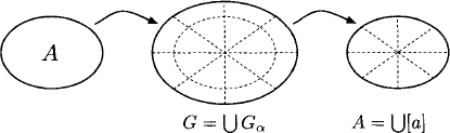
The result of the support decomposition of A is summarized in Figure E.1. The following definition given in (Kohlas & Wilson, 2006) is crucial since it summarizes all requirements for a semiring to give rise to a separative valuation algebra. Together with the requirement of a separative semigroup, it demands a decomposition that is monotonic under addition. This is needed to make allowance for the projection in equation (D.2), as shown beneath.
Figure E.1 A separative semigroup A is embedded into a semigroup G that consists of disjoint groups Gα. The support decomposition of A is then derived by denning two semigroup elements as equivalent if they belong to the same group Gα.
Definition E.4 A semiring ![]() is called separative, if
is called separative, if
- its multiplicative semigroup is separative,
- there is an embedding into a union of groups such that for all a,b
 A
A
The second condition expresses a kind of strengthening of positivity. This is the statement of the following lemma.
Lemma E.7 A separative semiring is positive.
Proof: From equation (E.2) we conclude [0] ≤ [a] for all a ![]() A. Then, assume a + b = 0. Hence, [0] ≤ [a],[b] ≤ [a + b] = [0] and consequently, a = b = 0.
A. Then, assume a + b = 0. Hence, [0] ≤ [a],[b] ≤ [a + b] = [0] and consequently, a = b = 0. ![]()
The following theorem states that a separative semiring is sufficient to guarantee that the induced valuation algebra is separative in the sense of Definition D.4.
Theorem E.8 Let ![]() be a valuation algebra induced by a separative semiring. Then
be a valuation algebra induced by a separative semiring. Then ![]() is separative.
is separative.
Proof: Since the semiring is separative, the same holds for the combination semigroup of Φ, i.e. ![]() = implies
= implies ![]() . Consequently, this semigroup can also be embedded into a semigroup that is a union of disjoint groups. In fact, the decomposition which is interesting for our purposes is the one induced by the decomposition of the underlying semiring. We say that
. Consequently, this semigroup can also be embedded into a semigroup that is a union of disjoint groups. In fact, the decomposition which is interesting for our purposes is the one induced by the decomposition of the underlying semiring. We say that ![]() , if
, if
This is clearly an equivalence relation Φ. Let ![]() and
and ![]() with
with ![]() and
and ![]() . Then, it follows that
. Then, it follows that ![]() and for all
and for all ![]() we have
we have
![]()
We therefore have a combination congruence in Φ. It then follows that the equivalence classes [![]() ] are subsemigroups of the combination semigroup of Φ.
] are subsemigroups of the combination semigroup of Φ.
Next, we define for a valuation ![]() the mapping
the mapping ![]() by
by
![]()
where Y is the semilattice of the group decomposition of the separative semiring. This mapping is well-defined since ![]() . We define for a valuation
. We define for a valuation ![]() with d(
with d(![]() ) = s
) = s
![]()
It follows that G[![]() ] is a group, if we define g × f by g × f(x) = g(x) × f(x), and the semigroup [
] is a group, if we define g × f by g × f(x) = g(x) × f(x), and the semigroup [![]() ] is embedded in it. The unit element f[
] is embedded in it. The unit element f[![]() ] of G[
] of G[![]() ] is given by f[
] is given by f[![]() ] (x) = fsP[
] (x) = fsP[![]() ](x) and the inverse of
](x) and the inverse of ![]() is defined by
is defined by ![]() -1(x) = (
-1(x) = (![]() (x))-1. This induces again a partial order
(x))-1. This induces again a partial order ![]() if
if ![]() for all x
for all x ![]() Ωs, or if
Ωs, or if ![]() . It is even a semilattice with
. It is even a semilattice with ![]() .
.
The union of these groups
![]()
is a commutative semigroup because, if ![]() and
and ![]() , then
, then ![]() is defined for
is defined for ![]() and
and ![]() by
by
![]()
and belongs to ![]() and is commutative as well as associative.
and is commutative as well as associative.
We have the equivalence ![]() because [
because [![]() ] is closed under combination.
] is closed under combination.
From equation (E.2) it follows that for ![]() and all
and all ![]() ,
,
![]()
This means that ![]() or also
or also
![]()
We thus derived the second requirement for a separative valuation algebra given in Definition D.4 for the congruence induced by the separative semiring. It remains to show that the cancellativity property holds in every equivalence class [![]() ]. Thus, assume
]. Thus, assume ![]() and for all
and for all ![]()
![]()
Since all elements ![]() and
and ![]() are contained in the same group, it follows that
are contained in the same group, it follows that ![]() by multiplication with
by multiplication with ![]() (x)-1. Therefore,
(x)-1. Therefore, ![]() which proves cancellativity of [
which proves cancellativity of [![]() ].
]. ![]()
Let us consider an example of a separative semiring and its induced valuation algebra. Subsequently, we then show that although separativity is again the weakest condition to allow for a division operation in the induced valuation algebra, there are still formalisms that do not even possess this structure.
![]() E.11 Arithmetic Potentials and Separativity
E.11 Arithmetic Potentials and Separativity
The particular arithmetic semiring of non-negative integers ![]() is separative and decomposes into the semigroups {0} and
is separative and decomposes into the semigroups {0} and ![]() . The first is already a trivial group, whereas
. The first is already a trivial group, whereas ![]() is embedded into the group of positive rational numbers. Note also that [0 × a] = [0], hence [0] ≤ [a] and [0] ≤ [0 + a] ≤ [a]. So, equation (E.2) holds. Thus, it induces a particular subalgebra of the valuation algebra of arithmetic potentials that is separative.
is embedded into the group of positive rational numbers. Note also that [0 × a] = [0], hence [0] ≤ [a] and [0] ≤ [0 + a] ≤ [a]. So, equation (E.2) holds. Thus, it induces a particular subalgebra of the valuation algebra of arithmetic potentials that is separative.
![]() E.12 Possibility Potentials and Separativity
E.12 Possibility Potentials and Separativity
The Lukasiewicz and drastic product t-norm semirings of Example 5.8 are not separative. Consequently, we cannot deduce anything about a possible division operation in their induced valuation algebras. This, however, does not hold for all t-norm semirings as shown in the following section.
E.2 REGULAR SEMIRING VALUATION ALGEBRAS
In the previous case, we exploited the fact that the multiplicative semigroup of a separative semiring can be embedded into a semigroup consisting of a union of disjoint groups. This allows introduction of a particular equivalence relation between semiring elements which in turn leads to a decomposition of the induced valuation algebra into cancellative semigroups with the corresponding congruence relation satisfying the requirement of a separative valuation algebra. In this section, we start with a semiring whose multiplicative semigroup decomposes directly into a union of groups. The mathematical requirement is captured by the following definition.
Definition E.5 A semigroup A with an operation × is called regular if for all a ![]() A there is an element b
A there is an element b ![]() A such that
A such that
![]()
Appendix D. 1.2 introduced the Green relation in the context of a regular valuation algebra and we learned that the corresponding congruence classes are directly groups. This technique can be generalized to regular semigroups. We define
![]()
and obtain a decomposition of A into disjoint congruence classes,
![]()
These classes are commutative groups under x, where every element a has a unique inverse denoted by a-1. Further, we write f[a] for the identity element in the group [a] and take up the partial order defined by f[a] ≤ f[b] if, and only if, f[a] × f[b] = f[a]. This is again a semilattice as we know from Section E.1. Finally, we obtain an induced partial order between the decomposition groups by [a] ≤ [b] if, and only if, f[a] ≤ f[b]. This is summarized in Figure E.2.
Definition E.6 A semiring ![]() is called regular if
is called regular if
- its multiplicative semigroup is regular,
- for all a,b
 A, [a] ≤ [a + b].
Figure E.2 A regular semigroup A decomposes directly into a union of disjoint groups using the Green relation.
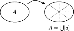
Theorem E.9 Let ![]() be a valuation algebra induced by a regular semiring. Then
be a valuation algebra induced by a regular semiring. Then ![]() is regular.
is regular.
Proof: Suppose ![]() with t
with t ![]() s = d(
s = d(![]() ) and
) and ![]() . We define
. We define
![]()
Then, it follows that for any x ![]() Ωs
Ωs
Here, the abbreviations f![]() and
and ![]() are used for f[
are used for f[![]() (x)] and
(x)] and ![]() respectively. Since the semiring is regular, we have [
respectively. Since the semiring is regular, we have [![]() (x)] ≤
(x)] ≤ ![]() and
and ![]() . Thus
. Thus
This proves the requirement of Definition D.5. •
We remark that regular semirings are also separative. Regularity of the multiplicative semigroup implies that every element in A has an inverse and we derive from a × a = a × b = b × b that a and b are contained in the same group of the semiring decomposition, i.e. [a] = [b]. Multiplying with the inverse of a gives then a = f[a] × b = b. This proves that the multiplicative semigroup of a regular semiring is separative. Requirement (E.2) follows from the strengthening of positivity in Definition E.6.
Let us again consider some concrete examples of regular semirings and their induced regular valuation algebra. As a confirmation of what we found out in Instance D.8, we first show that the arithmetic semiring is regular.
![]() E.13 Arithmetic Potentials and Regularity
E.13 Arithmetic Potentials and Regularity
The arithmetic semiring of non-negative real numbers is regular. It decomposes into a union of two disjoint groups ![]() and {0}, and we clearly have [0] ≤ [a] for all semiring elements a. Applying Theorem E.9 we conclude that its induced valuation algebra called arithmetic potentials is regular. However, we have also seen in Instance E. 11 that this property changes if we define the arithmetic semiring over different sets of numbers. On this note, the semiring view affords a whole family of valuation algebra instances that are closely related to arithmetic potentials but differ in their properties.
and {0}, and we clearly have [0] ≤ [a] for all semiring elements a. Applying Theorem E.9 we conclude that its induced valuation algebra called arithmetic potentials is regular. However, we have also seen in Instance E. 11 that this property changes if we define the arithmetic semiring over different sets of numbers. On this note, the semiring view affords a whole family of valuation algebra instances that are closely related to arithmetic potentials but differ in their properties.
![]() E.14 Probabilistic Constraints and Regularity
E.14 Probabilistic Constraints and Regularity
The t-norm semiring with usual multiplication as t-norm is regular too as we may deduce from the foregoing example. Therefore, its induced valuation algebra called probabilistic constraints is also regular. In fact, it is the only example of the t-norms listed in Example 5.8 that leads to a valuation algebra with a non-trivial division. The two t-norm discussed in Instance E. 12 do not allow division at all, and the minimum t-norm induces an idempotent valuation algebra as shown in Instance E.19 below.
![]() E.15 Spohn Potentials and Regularity
E.15 Spohn Potentials and Regularity
The tropical semiring ![]() is not regular because the solution b = -a of the regularity equation in Definition E.5 is not contained in the semiring. But if we extend the tropical semiring to all integers, then semiring is regular. The induced regular valuations of this extended semiring are called quasi-Spohn potentials.
is not regular because the solution b = -a of the regularity equation in Definition E.5 is not contained in the semiring. But if we extend the tropical semiring to all integers, then semiring is regular. The induced regular valuations of this extended semiring are called quasi-Spohn potentials.
E.3 CANCELLATIVE SEMIRING VALUATION ALGEBRAS
In Appendix E. 1, we started from a separative semigroup, which can be embedded into a semigroup consisting of a union of disjoint groups. Here, we discuss a special case in which the semigroup is embedded into a single group. The required property for the application of this technique is cancellativity. A semigroup A with operation × is called cancellative, if for a,b,c ![]() A,
A,
![]()
implies b = c. Such a semigroup can be embedded into a group G by application of essentially the same technique as in Appendix D.1.1. We consider pairs (a, b) of elements a, b ![]() A and define equality:
A and define equality:
![]()
Multiplication between pairs of semigroup elements is defined component-wise,
![]()
This operation is well-defined, since (a,b) = (a’,b’) and (c,d) = (c’,d’) implies (a,b) × (c,d) = (a’, b’) × (c’, d’). It is furthermore associative, commutative and the multiplicative unit e is given by the pairs (a,a) for all a ![]() A. Note that all these pairs are equal with respect to the above definition. We further have
A. Note that all these pairs are equal with respect to the above definition. We further have
![]()
which shows that (a,b) and (b,a) are inverses. Consequently, the set G of pairs (a,b) is a group into which A is embedded by the mapping a ![]() (a × a,a). If A itself has a unit, then 1
(a × a,a). If A itself has a unit, then 1 ![]() (1,1) = e. Without loss of generality, we may therefore consider A as a subset of G, This is summarized in Figure E.3.
(1,1) = e. Without loss of generality, we may therefore consider A as a subset of G, This is summarized in Figure E.3.
Figure E.3 A cancellative semigroup A is embedded into a group G consisting of pairs of elements from A.

Let us return to semirings and show how cancellative semirings induce valuation algebras with inverse elements.
Definition E.7 A semiring ![]() is called cancellative if its multiplicative semigroup is cancellative.
is called cancellative if its multiplicative semigroup is cancellative.
A cancellative semiring is also separative since from a × a = a × b it follows that a = b. We know that cancellative semirings can be embedded into a single group consisting of pairs of semiring elements, and since we have only one group, (E.2) is trivially fulfilled. Thus, cancellative semirings represent a particularly simple case of separative semirings and consequently induce separative valuation algebras due to Appendix E.1. We also point out that no direct relationship between cancellative and regular semirings exist. Cancellative semirings are embedded into a single group whereas regular semirings decompose into a union of groups. These considerations prove the following theorem:
Theorem E.10 Cancellative semirings induce separative valuation algebras.
We now examine an important example of a separative valuation algebra that is induced by a cancellative semiring.
![]() E.16 Weighted Constraints and Cancellativity
E.16 Weighted Constraints and Cancellativity
The tropical semiring of Example 5.4 is cancellative. Since the semiring values are non-negative and multiplication corresponds to addition, we always have that a × b = a × c implies b = c. To any pair of numbers a, b ![]() A we assign the difference a - b, which is not necessarily in the semiring anymore. In other words, the tropical semiring is embedded into the additive group of all integers.
A we assign the difference a - b, which is not necessarily in the semiring anymore. In other words, the tropical semiring is embedded into the additive group of all integers.
E.4 IDEMPOTENT SEMIRING VALUATION ALGEBRAS
Section 4.2.1 and Appendix D.1.3 introduced idempotency as a very strong additional condition. If this property is present in a valuation algebra, then every valuation becomes the inverse of itself, which allows us to simplify inference algorithms considerably. This lead to the very simple and time-efficient idempotent architecture of Section 4.5. Thus, we next go about studying which semiring properties give rise to idempotent valuation algebras.
Theorem E.11 c-semirings with idempotent multiplication induce idempotent valuation algebras.
Proof: From Lemma 5.6, (SP6) we conclude that
![]()
On the other hand, we have by Lemma 5.5, (SP4) and idempotency ![]()
![]()
This holds because ![]() (x) is a term of the sum. We therefore have
(x) is a term of the sum. We therefore have ![]() which proves idempotency.
which proves idempotency.
Idempotency of a semiring < A, +, x, 0,1 > directly implies the regularity of its multiplicative semigroup. Additionally, all groups [a] consist of a unique element as we learned in Appendix D.1.3. Since for all ![]() we have
we have
![]()
This implies [a] ≤ [a + b], from which we conclude that idempotent semirings are regular. Moreover, Lemma 5.5, (SP5) states that idempotent semirings are also positive which ensures the existence of neutral elements, null elements and stability in the induced valuation algebra as shown in Section 5.5.1 and 5.5.3. Altogether, this proves the following lemma:
Lemma E.8 c-semirings with idempotent × induce information algebras.
Theorem E.11 states that a c-semiring with idempotent multiplication is a sufficient condition for an idempotent semiring valuation algebra. It will next be shown that it is also necessary, if two additional conditions hold. In order to make a statement about all semiring elements starting from a semiring valuation algebra, all semiring elements must occur in the valuation algebra. In other words, Φ must be the set of all possible valuations taking values from a given semiring, whereas in other contexts it is often sufficient that Φ is only closed under combination and projection. The second condition excludes trivial lattices where the operation of projection has no effect.
Theorem E.12 Let ![]() be a semiring, r a set of variables and Φ the set of all possible semiring valuations defined over A and r. If <Φ, P(r)> is idempotent, then the semiring has idempotent multiplication. Moreover, if r contains at least one variable
be a semiring, r a set of variables and Φ the set of all possible semiring valuations defined over A and r. If <Φ, P(r)> is idempotent, then the semiring has idempotent multiplication. Moreover, if r contains at least one variable ![]() with |ΩX| > 1, then the semiring is also a c-semiring.
with |ΩX| > 1, then the semiring is also a c-semiring.
Proof: Since Φ is the set of all possible valuations, there exists a for all a ![]() A a valuation
A a valuation ![]() with
with ![]() . Idempotency implies that
. Idempotency implies that
![]()
We therefore have a × a = a for all a ![]() A with proves idempotency of semiring multiplication. Next, assume that there exists X
A with proves idempotency of semiring multiplication. Next, assume that there exists X ![]() r with ΩX = {x1, x2, …, xn}. For all a
r with ΩX = {x1, x2, …, xn}. For all a ![]() A, we then have a valuation
A, we then have a valuation ![]() with d(Ψ) = {X} and
with d(Ψ) = {X} and ![]() (x1) = 1,
(x1) = 1, ![]() (x2) = a and
(x2) = a and ![]() (xi) = 0 for all i > 2. Idempotency implies that
(xi) = 0 for all i > 2. Idempotency implies that
![]()
This shows that the semiring is a c-semiring. ![]()
Let us again consider some examples of c-semirings with idempotent multiplication and their induced information algebras. First, we apply this analysis to the Boolean semiring to confirm what we have found out in Instance 4.2.
![]() E.17 Indicator Functions and Idempotency
E.17 Indicator Functions and Idempotency
It has been shown in Example 5.10 that the Boolean semiring is a c-semiring. Since multiplication corresponds to minimization, this semiring is also idem-potent. We therefore conclude from Lemma E.8, the induced valuation algebra of indicator functions must be an information algebra.
![]() E.18 Bottleneck Constraints and Idempotency
E.18 Bottleneck Constraints and Idempotency
The bottleneck semiring of Example 5.3 is clearly a c-semiring with idempotent multiplication. Its induced valuation algebra is therefore another example of an information algebra.
![]() E.19 Possibility Potentials and Idempotency
E.19 Possibility Potentials and Idempotency
We already pointed out in Example 5.10 that all t-norm semirings are c-semirings. However, only the minimum t-norm among them is idempotent which again turns its induced valuation algebra into an information algebra. This example is very similar to the Bottleneck constraints above.
A summary of the division-related properties of different semiring valuation algebras is shown in Figure E.4.
E.5 SCALABLE SEMIRING VALUATION ALGEBRAS
As a last complement on division for semiring valuation algebras, we recall from Section 4.7 that scaling or normalization may be an important semantical issue for some valuation algebras. The algebraic requirement that makes scaling possible is separativity. Thus, we may conclude that separative semirings induce valuation algebra with scaling if there exists a semantical need for this operation. Among the instances discussed in this appendix, we have seen that the arithmetic semiring is regular and allows scaling in its induced valuation algebra. This leads again to the probability potentials introduced in Instance 4.4. Here are two further examples of scalable valuation algebras:
Figure E.4 Semiring valuation algebras and division-related properties.

![]() E.20 Normalized Weighted Constraints
E.20 Normalized Weighted Constraints
Weighted constraints are induced by the cancellative tropical semiring and are therefore separative. According to equation (4.29), the scale of a weighted constraint c ![]() is given by
is given by
![]()
This operation ensures that the minimum weight is always zero.
![]() E.21 Normalized Probabilistic Constraints
E.21 Normalized Probabilistic Constraints
The product t-norm semiring induces probabilistic constraints which naturally explains the interest in scaling. This semiring is regular and therefore also fulfills the algebraic requirement. According to equation (4.29), the scale of the probabilistic potential ![]() is given by
is given by
![]()
PROBLEM SETS AND EXERCISES
E.1* Section 5.6 shows that the space complexity of the Shenoy-Shafer architecture of equation (4.9) can be improved when dealing with semiring valuations. Think about a similar improvement for set-based semiring valuation algebras.
E.2* Consider mappings from singleton configuration sets to the values of a commutative semiring and prove that they form a subalgebra of the valuation algebra of set-based semiring valuations. Identify the requirements for neutral and null elements and observe that neutral elements are different in the two algebras. Compare the results with usual semiring valuations.
E.3* Exercise D.4 in Chapter 4 introduced a partial order between valuations in an information algebra. We-know from Lemma E.8 that c-semirings with idempotent × induce information algebras. How is the semiring order of equation (5.4) related to the partial order between valuations in the induced information algebra?
E.4* We claim in Example 5.8 and 5.10 that < [0,1], max, x, 0,1 > always forms a c-semiring when an arbitrary t-norm is taken for multiplication. Prove this statement. The definition of a t-norm requires that the number 1 is the unit element. Without this condition the structure it is called a uninorm. Prove that we still obtain a semiring, albeit not a c-semiring, when a uninorm is taken instead of a t-norm. Finally, show that we may also replace maximization for semiring addition by an arbitrary uninorm.
E.5** Exercise D.8 in Chapter 4 introduced conditionals ![]() s|t for disjoint sets s,t
s|t for disjoint sets s,t ![]() d(
d(![]() ) in regular valuation algebras
) in regular valuation algebras ![]() .
.
a) Identify the conditionals in the valuation algebras of probabilistic constraints from Instance 5.2 and quasi-Spohn potentials of Instance E.15.
b) Prove that if ![]() and
and ![]() are disjoint sets we have
are disjoint sets we have
c) Convince yourself that the arctic semiring is regular and therefore also the induced valuation algebra of GAI preferences from Instance 5.1. Show that equation (E.3) corresponds to Bellman’s principle of optimality (Bellman, 1957) when it is expressed in the valuation algebra of GAI preferences.
The solution to these exercises is given in Section 5.2 of (Kohlas, 2003).
E.6** Identify the algebraic properties (i.e. division, neutral and null elements) for the valuation algebras induced by the t-norm semirings with the following t-norms:
1. Nil-potent maximum: For a, b ![]() [0,1]
[0,1]
2. Hamacher product: For a, b ![]() [0,1]
[0,1]
E.7*** Exercise E.4 defines a uninorm as a generalization of a t-norm where the unit element does not necessarily correspond to the number 1. If we have a uninorm with the number 0 as unit element, then it is called a t-conorm. We directly conclude from Exercise E.4 that we obtain a semiring when we take a t-conorm for multiplication and maximization for addition. Give a t-norm T and a, b ![]() [0,1], we define its associated t-conorm by
[0,1], we define its associated t-conorm by
(E.4) ![]()
Is it possible to conclude the form of division in a valuation algebra induced by a t-conorm semiring from the form of division that is present in the valuation algebra induced by the corresponding t-norm semiring?
E.8*** Instance D.6 shows that the valuation algebra of set potentials is separative. Generalize these considerations to set-based semiring valuations and identify the algebraic requirements for a semiring to induce separative, regular and idempotent set-based semiring valuation algebras.