CHAPTER 6

VALUATION ALGEBRAS FOR PATH PROBLEMS

Together with semiring constraint systems introduced in Chapter 5, the solution of path problems in graphs surely ranks among the most popular and important application fields of semiring theory in computer science. In fact, the history of research in path problems strongly resembles that of valuation algebras and local computation in its search for genericity and generality. In the beginning, people studied specific path problems which quickly brought out a large number of seemingly different algorithms. Based on this research, it was then observed that path problems often provide a common algebraic structure. This gave birth of an abstract framework called algebraic path problem which unifies the formerly isolated tasks. Typical instances of this framework include the computation of shortest distances, maximum capacities or reliabilities, but also other problems that are not directly related to graphs such as partial differentiation or the determination of the language accepted by a finite automaton. This common algebraic viewpoint initiated the development of generic procedures for the solution of the algebraic path problem, similar to our strategy of defining generic local computation architectures for the solution of inference problems. Since the algebraic path problem is not limited to graph related applications, its definition is based on a matrix of semiring values instead. We will show in this chapter that depending on the semiring properties, such matrices induce valuation algebras. This has several important consequences: on the one hand, we then know that matrices over special families of semirings provide further generic constructions that deliver many new valuation algebra instances. These instances are very different from the semiring valuation algebras of Chapter 5, because they are subject to a pure polynomial time and space complexity. On the other hand, we will see in Chapter 9 that inference problems over such valuation algebras model path problems that directly enables their solution by local computation. This comes along with many existing approaches that focus on solving path problems by sparse matrix techniques.

The first section introduces the algebraic path problem from a topological perspective and later points out an alternative description as a particular solution to a fixpoint equation, which generally is more adequate for an algebraic manipulation. Section 6.3 then discusses quasi-regular semirings that always guarantee the existence of at least one solution to this equation. Moreover, it will be shown that a particular quasi-inverse matrix can be computed from the quasi-inverses of the underlying semiring. This leads in Section 6.4 to the first generic construction related to the solution of path problems. Since quasi-regular semirings are very general and only possess little algebraic structure, it will be remarked in Section 6.5 that the same holds for their induced valuation algebras. We therefore present in Section 6.6 a special family of quasi-regular semirings called Kleene algebras that uncover a second generic construction related to path problems in Section 6.7. This approach always leads to idempotent valuation algebras and also distinguishes itself in other important aspects from quasi-regular valuation algebras, as pointed out in Section 6.8.

6.1 SOME PATH PROBLEM EXAMPLES

The algebraic path problem establishes the connection between semiring theory and path problems. To motivate a closer investigation of this combination, let us first look at some typical examples of path problems.

6.1 The Connectivity Problem

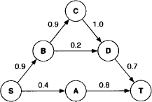
The graph of Figure 6.1 represents a traffic network where nodes model junctions and arrows one-way streets. Every street is labeled with a Boolean value where 1 stands for an accessible street and 0 for a blocked street due to construction works. The connectivity problem now asks the question whether node T can still be reached from node S. This is computed by taking the maximum value over all possible paths leading from S to T, where the value of a path corresponds to the minimum of all its edge values. We compute for the three possible paths from S to T:

and then

Thus, node T can still be reached from node S.

6.2 The Shortest and Longest Distance Problem

A similar traffic network is shown in Figure 6.2. This time, however, edges are labeled with natural numbers to express the distance between neighboring nodes. The shortest distance problem then asks for the minimum distance between node S and node T, which corresponds to the minimum value of all possible paths leading from S to T, where the value of a path consists of the sum of all its edge values. We compute

and then

Thus, the shortest distance from node S to node T is 11. We could also replace minimization by maximization to determine the longest or most critical path.

6.3 The Maximum Capacity Problem

Let us next interpret Figure 6.3 as a communication network where edges represent communication channels between network hosts. Every channel is labeled with its capacity. The maximum capacity problem requires to compute the maximum capacity of the communication path between node S and node T, where the capacity of a communication path is determined by the minimum capacity over all channels in this path. Similar to Instance 6.1 we compute

Thus, the maximum capacity over all channels connecting S and T is 3.6.

6.4 The Maximum Reliability Problem

We again consider Figure 6.4 as a communication network where edges represent communication channels. Such channels may fail and are therefore labeled with a probability value to express their probability of availability. Thus, we are interested in the most reliable communication path between node S and node T, where the reliability of a path is obtained by multiplying all its channel probabilities. We compute

and then

Thus, the most reliable communication path has a reliability of 0.567.

6.5 The Language of an Automaton

Finally, we consider the automaton of Figure 6.5 where nodes represent states, and the edge values input words that bring the automaton into the neighbor state. Here, the task consists in determining the language that brings the automaton from state S to T. This is achieved by collecting the strings of each path from S to T, which are obtained by concatenating their edge values. We compute

and then

Thus, the language that brings the automaton from state S to T is {ac, aba, acba}.

Further examples of path problems will be given at the end of this chapter.

6.2 THE ALGEBRAIC PATH PROBLEM

We next introduce a common formal background of these well-known path problems: Consider a weighted, directed graph (V, E, A, w) where (V, E) is a directed graph and ω a weight function that assigns a value from an arbitrary semiring A, +, x, 0, 1 to each edge of the graph, ω: E → A. If p = (V0, …, Vn) denotes a path of length n between a source node S = V0 and a target node T = Vn, the path weight w(p) is denned as the product of all semiring values that are assigned to its edges,

(6.1)

Since we later identify graph nodes with variables, we here use capital letters to refer to graph nodes. It is important to note that we assumed an arbitrary semiring where multiplication is not necessarily commutative, which forces us to mind the order of multiplication. Also, many paths between S and T may exist. We write PS,T for the set of all possible paths connecting a source S with a terminal T. Solving the path problem for S T then consists in computing

(6.2)

If S = T we simply define D(S, T) = 1 as the weight of the empty path. This is the unit element of the semiring with respect to multiplication and ensures that path weights are not affected by cycling an arbitrary number of times within an intermediate node. If no path exists between the two nodes S and T, equation (6.2) sums over the empty set which, by definition, returns the zero element of the semiring. Alternatively, we may define PS,Tr as the set of all paths from node S to node T of length r ≥ 0. We obtain

and consequently for S T

(6.3)

Example 6.1 The connectivity problem of Instance 6.1 is based on the Boolean semiring of Example 5.2. Finding shortest distances according to Instance 6.2 amounts to computing in the tropical semiring of Example 5.4 where semiring multiplication corresponds to addition and semiring addition to minimization. The maximum capacity problem of Instance 6.3 is induced by the bottleneck semiring of Example 5.3, and the product t-norm semiring of Example 5.8 allows to compute the most reliable path in Instance 6.4. Finally, the language of the automaton in Instance 6.5 is computed by the semiring of regular languages of Example 5.7. Observe that this semiring is not commutative.

There are several critical points regarding the equations (6.2) and (6.3): First, these formulas is entirely based on a graph related conception due to the explicit use of a path set. This may be sufficient for the examples given above, but we already pointed out in the introduction of this chapter that other applications without this interpretation exist. Second, it may well be that an infinite number of paths between two nodes exists, as it is for example the case in graphs with cycles. We then obtain an infinite sum in both equations that is not necessarily defined. These are the two major topics for the remaining part of this section. To start with, we develop a more general definition of path problems based on semiring matrices instead of path sets.

Example 6.2 The graph in Figure 6.6 contains a cycle between the nodes 1 and 6. The path set P1,6 therefore contains an infinite number of paths. Depending on the semiring, the sum in equation (6.2) is not defined.

From now on, we again identify graph nodes with natural numbers {1, …, n} with n = |V|. The advantage of this convention is that we may represent a weighted graph in terms of its adjacency matrix M M(A, n) defined as follows:

(6.4)

Due to the particular node numbering, the matrix entries directly identify the edge weights in the graph. It is sometimes common to set the diagonal elements of this semiring matrix to the unit element 1, if no other weight is specified in the graph. This, however, is not necessary for our purposes. Note that an adjacency matrix describes a full graph where any two nodes are linked, although some edges have weight zero. As a consequence, any sequence of nodes describes a path, but only the paths of weight different from zero describe paths in the underlying graph. Also, the definition of an adjacency matrix excludes multigraphs where multiple edges with identical directions but different weights may exist between two nodes. But this can be taken into consideration by assigning the sum of all weights of edges leading from node X to y to M (X, Y).

Example 6.3 Figure 6.7 shows a directed, weighted graph defined over the tropical semiring and its associated adjacency matrix. Unknown distances are set to the zero element of the semiring, which here corresponds to ∞.

The solution of path problems based on adjacency matrices uses semiring matrix addition and multiplication as introduced in Section 5.1.2. Remember that matrices over semirings form themselves a semiring with the identity matrix as unit and the zero matrix as zero element. Let us next consider the successive powers of the adjacency matrix:

and more generally

We immediately observe that Mr (S, T) corresponds to the sum of all path weights of length r between the selected source and target node. It therefore holds that

and we obtain the sum of all path weights of length at most r ≥ 0 by

(6.5)

The identity matrix handles paths of length 0 by defining I(X, Y) = M(0) (X, Y) = 1 if X = Y and I(X, Y) = M(0)(X, Y) = 0 otherwise. Its importance will be illustrated in Example 6.4 below. For r > 0, this sum of matrix powers can also be seen as the sum of the weights of all paths between S and T that visit at most r - 1 intermediate nodes. We are tempted to express the matrix D of equation (6.3) as the infinite sum

(6.6)

This corresponds to the sum of all paths between S and T visiting an arbitrary and unrestricted number of nodes. Contrary to equation (6.3) we have now derived a description of path problems that is independent of path sets and therefore not restricted to graph based applications anymore. On the other hand, we still face the problem of infinite sums of semiring values. Subsequently, we therefore introduce a topology on partially ordered semirings that allows us to define and study such formal sequences.

Example 6.4 We reconsider the adjacency matrix from Example 6.3 and compute its successive powers for 1 ≤ r ≤ 4 based on the tropical semiring with addition for semiring multiplication and minimization for semiring addition.

M4(1, 3) = 28 for example means that the distance of the shortest path from node 1 to node 3 containing exactly 4 edges is 28. Using equation (6.5) we compute M(4) that contains all shortest paths of at most 4 edges:

M(4) = I + M + M2 + M3 + M4

Here, M(4)(1, 3) = 8 means that the distance of the shortest path from node 1 to node 3 containing at most 4 edges is 8. In this very special case, M(4) already contains all shortest paths in the graph of Figure 6.7 which is not generally the case. Also, we observe the importance of the identity matrix to ensure that each node can reach itself with a shortest distance of 0.

We next generalize the power sequence of semiring matrices to arbitrary semirings A and define for r ≥ 0 and a A:

(6.7)

The following recursions are direct consequences of this definition:

(6.8)

From Lemma 5.2, (SP3) follows that the power sequence is non-decreasing,

(6.9)

This refers to the canonical preorder of semirings introduced in equation (5.3). We also remember that if this relation is a partial order, the semiring is called a dioid. Idempotency of addition is always a sufficient condition to turn the preorder into a partial order which then is equivalently expressed by equation (5.4). Following (Béeatréma, 1982) dioids can be equipped with a particular topology called sup-topology, where a sequence of dioid values is convergent, if it is non-decreasing, bounded from above and if it has a least upper bound. The limit of a convergent sequence then corresponds to its least upper bound. However, the simple presence of the sup-topology is not yet sufficient for our purposes. Instead, two additional properties must hold which are summarized in the definition of a topological dioid (Gondran & Minoux, 2008).

Definition 6.1 A dioid endowed with the sup-topology with respect to its canonical partial order is called topological dioid if the following properties hold:

Thus, if the semiring is a topological dioid and if the power sequence is bounded from above, it follows from Definition 6.1 that the sequence has a least upper bound. We then know that the sequence is convergent with respect to the sup-topology and that its limit corresponds to the least upper bound. We subsequently denote the limit of the power sequence by

(6.10)

Example 6.5 Bounded semirings of Definition 5.3 satisfy a + 1 = 1 for all a A. They are idempotent since 1 + 1 = 1 always implies that a + a = a. Thus, bounded semirings are dioids, and since a ≤ 1 we also have ar ≤ 1 and therefore a(r) = 1 + a + … + ar ≤ 1. This shows that power sequences over bounded semirings are always non-decreasing and bounded from above. If we further have a topological dioid, then the limit of this sequence exists for each a A. Some instances of bounded semirings were given in Example 5.10.

The following theorem links the limit of a power sequence in a topological dioid to the solution of a linear fixpoint equation. Semiring elements that satisfy this equation are generally referred to as quasi-inverses. Note that we subsequently write ab for a × b whenever it is contextually clear that we refer to semiring multiplication. Also, we keep our convention to refer to variables by capital letters.

Theorem 6.1 If a* exists in a topological dioid, it is always the least solution to the fixpoint equations

(6.11)

Let us first prove the following intermediate result:

Lemma 6.1 Let A be an arbitrary semiring and y A a solution to (6.11). We have

(6.12)

and the solution y is an upper bound for the sequence a(r).

Proof: We proceed by induction: For r = 0 we have y = ay + 1. This holds because y is a solution to equation (6.11). Assume now that equation (6.12) holds for r. For r + 1 it then follows from equation (6.8) and the induction hypothesis that

Using Lemma 5.2, (SP3) we finally conclude that a(r) ≤ y.

Using this result we next prove Theorem 6.1:

Proof: Taking the limit in a topological dioid is compatible with semiring addition and multiplication. We thus conclude that the limit of aa(r) is aa* and that aa(r) + 1 is convergent with limit aa* + 1. It follows from equation (6.8) that a* = aa* + 1 and similarly that a* = a*a + 1. This shows that a* is a solution to equation (6.11). From Lemma 6.1 follows that for all solutions y we have a(r) ≤ y. Due to equation (6.10) the particular solution a* is the least upper bound of the power sequence and therefore also the least solution to both fixpoint equations.

There may be several solutions to these fixpoint equations and thus several quasi-inverses for a semiring element as shown in Example 6.6 below. But if we have a topological dioid where the power sequence converges, then its limit is the least element among them. Further, we show in Lemma 6.2 below that the limit also determines the least solution to more general fixpoint equations.

Example 6.6 Consider the tropical semiring , min, of Example 5.4. We then obtain for equation (6.11) x = min{a + x, 0}. For a > 0 this equation always has a unique solution x = 0. If a < 0 there is no solution and if a = 0, then every x ≤ 0 is a solution to this fixpoint equation.

Lemma 6.2

Proof:

Let us return to the solution of path problems and the power sequence of semiring matrices in equation (6.6). We first recall that matrices with values from a semiring themselves form a semiring with a component-wise definition of the canonical pre-order. Thus, if this relation is a partial order, then the corresponding semiring of matrices is also a dioid. Moreover, if the semiring is a topological dioid, then so is the semiring of matrices (Gondran & Minoux, 2008). We conclude from equation (6.10) that if the power sequence of semiring matrices with values from a topological dioid converges, then solving a path problem is equivalent to computing the least quasi-inverse matrix. This computational task is stated by the following definition:

Definition 6.2 Let M M(A, n) be a square matrix over a topological dioid A. If the limit exists, the algebraic path problem consists in computing

(6.13)

We now have a formally correct and general description of a path problem that is not restricted to graph related applications anymore. However, it is based on the limit of an infinite sequence and therefore rather inconvenient for computational purposes. An alternative way to express the algebraic path problem by means of the least solution to a linear fixpoint equation is indicated by Theorem 6.1. For that purpose, we first derive a converse result to this theorem:

Lemma 6.3 If in a topological dioid y is the least solution to the fixpoint equations

(6.14)

then it corresponds to the quasi-inverse of a A satisfying

Proof: We recall from equation (6.9) that the sequence a(r) is non-decreasing. Further, because we have assumed the existence of a least solution, the sequence is also bounded by Lemma 6.1. Definition 6.1 then assures that the sequence has a least upper bound which corresponds to the limit of the power sequence. But then, this limit is the least solution to the fixpoint equation according to Theorem 6.1 and corresponds to y since the least element is uniquely determined.

We obtain from Theorem 6.1 and Lemma 6.3 the following alternative but equivalent definition of the algebraic path problem:

Definition 6.3 Let M M(A, n) be a square matrix over a topological dioid A. The algebraic path problem consists in computing the least solution to

(6.15)

if such a solution exists.

Here, the variable X refers to an unknown matrix in M(A, n). It is important to note that this definition is still conditioned on the existence of a solution, respectively on the convergence of the power sequence. Imagine for example that we solve a shortest distance problem on the cyclic graph of Figure 6.6 with negative values assigned to the edges of the cycle. If we then consider the path weights between the source and target node, we obtain a shorter total distance for each additional rotation in the cycle. In this case, the limit of equation (6.13) does not exist or, in other words, the fixpoint equations have no solution. This is comparable to the case a < 0 in Example 6.6. Investigating the requirements for the existence of quasi-inverses is an ongoing research topic. Many approaches impose restrictions on graphs which for example forbid cycles of negative path weights in case of the shortest distance problem. But this naturally only captures graph related applications. Alternatively, we may ensure the existence of quasi-inverses axiomatically which also covers other applications. Then, the semiring of Example 6.6, where no quasi-inverses exist for negative elements, would not be part of the framework anymore. However, we can easily imagine that shortest distances can still be found in graphs with negative values, as long as there are no cycles with negative path weights. In many cases we can adjoin an additional element to the semiring that acts as an artificial limit for those sequences that are divergent in the original semiring. Reconsider the shortest distance problem with edge weights from the semiring , min, +, . Here, it is reasonable to define M*(S, T) = -∞, if the path from node S to T contains a cycle of negative weight. This amounts to computing in the extended semiring , min, +, with . Then, the problem of non-existence in Definition 6.3 is avoided and the algebraic path problem reduces to finding a particular solution to a semiring fixpoint equation.

6.3 QUASI-REGULAR SEMIRINGS

We now focus on semirings where each element has at least one quasi-inverse. Then, it is always possible to introduce a third semiring operation called star operation that delivers a particular quasi-inverse for each semiring element. Such semirings are called closed semirings in (Lehmann, 1976) but to avoid confusions with other semiring structures, we prefer to call them quasi-regular semirings.

Definition 6.4 A quasi-regular semiring A, +, x, *, 0, 1 is an algebraic structure where A, +, x, 0, 1 is a semiring and * an unary operation such that for a A

Restricting Example 6.6 to non-negative integers, we see that quasi-inverse elements are not necessarily unique in a semiring. Consequently, there may be different ways of defining the star operation which each time leads to a different quasi-regular semiring. Here, we list some possible extensions to quasi-regular semirings for the examples that marked the beginning of this chapter:

Example 6.7 The tropical semiring of non-negative real numbers (or integers) introduced in Example 5.4 is quasi-regular with a* = 0 for all a . This can be extended to the tropical semiring of all real numbers , min, +, by a* = 0 for a ≥ 0 and a* = -∞ for a < 0. Similarly, the arctic semiring from Example 5.5 , max, is quasi-regular with a* = ∞ for a ≥ 0 and a* = 0 for a . The Boolean semiring {0, 1}, max, min, 0, 1 of Example 5.2 is quasi-regular with 0* = 1* = 1. This also holds for the bottleneck semiring , max, min, from Example 5.3 where a* = for all elements. The probabilistic or product t-norm semiring [0, 1], max, ˙, 0, 1 of Example 5.8 is extended to a quasi-regular semiring by defining a* = 1 for all a [0, 1]. Finally, the semiring of formal languages presented in Example 5.7 is quasi-regular with

(6.16)

Example 6.1 showed that these semirings were used in the introductory path problems of this chapter which are thus based on quasi-regular semirings.

If we consider matrices with values from a quasi-regular semiring, then it is possible to derive quasi-inverse matrices from the star operation in the underlying semiring through the following induction:

• For n = 1 we define [a]* = [a*].
• For n > 1 we decompose the matrix M into submatrices B, C, D, E such that B and E are square and define

(6.17)

where F = E + DB*C.

It is important to note that equation (6.17) does not depend on the way how the matrix M is decomposed. This can easily be proved by applying equation (6.17) to a matrix with nine submatrices, decomposed in two different ways:

and

and by verifying nine identities using the semiring properties from Definition 5.1. A graph based justification of equation (6.17) will later be given in Example 6.12. The following theorem has been proposed by (Lehmann, 1976):

Theorem 6.2 Let be a matrix with values from a quasi-regular semiring A. Then, the matrix M* obtained from equation (6.17) satisfies

(6.18)

Proof: Because the two equalities in (6.18) are symmetric we only prove the first one. Let us proceed by induction: For n = 1 the equality holds by Definition 6.4. The induction hypothesis is that equation (6.18) holds for matrices of size less than n. For n > 1 suppose the decomposition

with for some n > k > 0. By equation (6.17) we have

and therefore

By the induction hypothesis we have

This together with F = E + DB*C gives us the following four equalities:

We finally obtain

Thus, given a quasi-regular semiring, we can find a quasi-inverse for each matrix defined over this semiring. In other words, each quasi-regular semiring induces a particular quasi-regular semiring of matrices through the above construction. Algorithms to compute such quasi-inverse matrices will be presented in Chapter 9. Here, we benefit from this important result to reformulate the algebraic path problem of Definition 6.3 for matrices over quasi-regular semirings.

Definition 6.5 For a matrix M M(A, n) over a quasi-regular semiring A, the algebraic path problem consists in computing M* defined by equation (6.17).

It is important to note that the two Definitions 6.3 and 6.5 of the algebraic path problem are not equivalent and in fact difficult to compare. We mentioned several times that quasi-inverses do not need to be unique. Definition 6.3 presupposes a partial order and focusses on the computation of the least quasi-inverse with respect to this order. Quasi-regular semirings do not necessarily provide a partial order such that we obtain an arbitrary quasi-inverse from solving the algebraic path problem in Definition 6.5. But even if we assume a partial order in the quasi-regular semiring of Definition 6.5 and also that all sequences in Definition 6.3 converge (Aho et al., 1974), we do not necessarily have equality between the two quasi-inverses (Kozen, 1990). We can therefore only observe that a solution to the algebraic path problem with respect to Definition 6.5 always satisfies the fixpoint equation of Theorem 6.1, although it is not necessarily the least element of the solution set. In Section 6.6 we will introduce a further semiring structure that extends quasi-regular semirings by idempotency and also adds a monotonicity property with respect to the star operation. In this setting, the quasi-inverse matrix obtained from equation (6.17) will again be the least solution to the fixpoint equation. We will now give an example of a quasi-inverse matrix which is obtained from the above construction:

Example 6.8 We have seen in Example 6.7 that the tropical semiring of non-negative integers , min, +, is quasi-regular with a* = 0 for all a . Let us assume the following matrix defined over this semiring and compute its quasi-inverse by equation (6.17). The following decomposition is chosen:

With semiring addition as minimization, semiring multiplication as integer addition and ∞* = 0 we first compute

Applying equation (6.17) we obtain

Since B* = [0] we directly conclude

and compute for the two remaining submatrices:

Putting these results together, we obtain the quasi-inverse matrix M*:

If we interpret M as a distance matrix, we immediately observe that M* contains all shortest distances. An explanation why the above construction for quasi-inverse matrices always leads to shortest distances in case of the tropical semiring over non-negative numbers will be given in Section 6.6.

To conclude this section, Example 6.9 alludes to an alternative way of deriving the fixpoint equation of Definition 6.5 which is not motivated by the semiring power sequence, but instead uses Bellmann’s principle of optimality (Bellman, 1957).

Example 6.9 Let M be the adjacency matrix of a directed, weighted graph with edge weights from the tropical semiring , min, +, of non-negative integers. We may then write equation (6.18) for X Y such that B(X, Y) = ∞ as

Similarly, we obtain for X = Y

The first equation states that the shortest path from node X to node Y corresponds to the minimum sum of the direct distance to an intermediate node Z and the shortest path from Z to the terminal node Y. This is Bellmann’s principle of optimality. The second equality states that each node can reach itself with distance zero.

The complete matrix M* of Example 6.9 contains the shortest distances between all pairs of graph nodes. It is therefore common to refer to the generalized computational task of Definition 6.3 as the all-pairs algebraic path problem. If we are only interested in the shortest distances between a selected source node S and all possible target nodes, it is sufficient to compute the row of the matrix M* that corresponds to this source node, i.e. we compute bM* where b is a row vector with b(S) = 1 and b(Y) = 0 for all Y S. It then follows from M* = MM* + I that bM* = bMM* + b. This shows that bM* is a solution to

(6.19)

where X is a variable row vector. Hence, we refer to the task of computing bM* defined by equation (6.17) as the single-source algebraic path problem. In a similar manner, the column vector M*b is a solution to

(6.20)

and refers in the above instantiation to the shortest distances between all possible source nodes and the selected target node. The task of computing equation M*b defined by equation (6.17) is therefore called single-target algebraic path problem. Clearly, instead of solving the all-pairs problem directly, we can either solve the single-source or single-target problem for each possible vector b, i.e. for each possible source or target node. We will see in the following section that matrices over quasi-regular semirings induce a family of valuation algebras called quasi-regular valuation algebras. It will be shown in Chapter 9 that the single-source algebraic path problem can be solved by local computation with quasi-regular valuation algebras.

6.4 QUASI-REGULAR VALUATION ALGEBRAS

In this section, we are going to derive a generic construction that leads to a new valuation algebra for each quasi-regular semiring. These formalisms, called quasi-regular valuation algebras, are related to the solution of the single-target algebraic path problem or, in other words, to the computation of a single column of the quasi-inverse matrix that results from equation (6.17). Until now, we have dealt in this chapter with ordinary semiring matrices. But for the study of generic constructions and valuation algebras, we will reconsider labeled matrices as introduced in Chapter 1 for real numbers. This time, however, we assume labeled matrices with values from a quasi-regular semiring A. Thus, let r be a set of variables, and M(A, s) the set of labeled matrices M: . Inspired by (Lehmann, 1976; Radhakrishnan et al., 1992; Backhouse & Carré, 1975), we observe that the pair (M, b) for M M(A, s) and an s-vector b: s → A sets up the fixpoint equation

(6.21)

where X denotes a variable column vector with domain s. This equation can be regarded as a labeled version of equation (6.20) generalized to vectors b of arbitrary values from a quasi-regular semiring. We further define the set

(6.22)

and also write d(M, b) = s if M M(A, s).

In order to introduce a projection operator for the elements in Φ, we first decompose the above system with respect t s and obtain

from which we derive the two equations

and

Lemma 6.2 points out that with

provides a solution to the first equation. Note, however, that is not a semiring value, so that our discussion so far is only informal. Nevertheless, let us proceed with this expression and insert it into the second equation. After regrouping of variables we obtain

For (M, b) with d(M, b) = s and t ⊆ s this indicates that we could define

(6.23)

with

(6.24)

and

(6.25)

such that

The following theorem justifies this informal argument. It states that if a particular solution to equation (6.21) is given, then the restriction of this solution to the subdomain also solves the projected equation system. Conversely, it is always possible to reconstruct the solution to the original system from the projected solution.

Theorem 6.3 For a quasi-regular semiring A with M M(A, s), b: s → A and t ⊆ s, the following statements hold:

then (y, x) = M*b is a solution to X = MX + b.

Proof:

1. We first consider the submatrices of M* with respect to s - t and t. From

we derive the following identity using equation (6.17) and (6.24):

and then further:

(6.28)

If × = M*b is a solution to X = MX + b we have

Decomposing the system with respect to s - t and t gives

We identify the following subsystem for t:

If we insert the above identities for the left-hand side of this equation, we obtain

This follows from equation (6.25). Similarly, we obtain for the right-hand part:

Reordering the terms of this expression gives:

The last equality follows from equations (6.24) and (6.25).

which by Lemma 6.2 proves that (Mt)*bt is a solution to

This proves the first statement of the theorem.

2. It follows from equations (6.25) and (6.28) that

Similarly, we derive

We therefore obtain:

But according to Lemma 6.2 M*b is always a solution to the fixpoint equation

This proves the second statement of the theorem.

Subsequently, we use to say that x is a solution to (M, b) if x is a solution to the fixpoint equation X = MX + b. The following lemma highlights a direct consequence of the above theorem:

Lemma 6.4 If x = M*b is a solution to (M, b) and t ⊆ s = d(M, b) then

Proof: If M*b is a solution to (M, b), then (Mt)*bt and (Ms-t)*bs-t are solutions to (Mt, bt) and (Ms-t, bs-t) by the first statement of Theorem 6.3. On the other hand, if (Mt)*bt is a solution to (Mt, bt) and

then ((Mt)*bt, y1) = M*b, which follows from the second statement of Theorem 6.3. Likewise, if (Ms-t)*bs-t is a solution to (Ms-t, bs-t), there exists an extension y2 such that (y2, (Ms-t)*bs-t) = M*b. We conclude from

that y1 = (Ms-t)*bs-t and y2 = (Mt)*bt.

We next prove that the projection operator is transitive.

Lemma 6.5 For (M, b) with d(M, b) = s and t ⊆ u ⊆ s we have

(6.29)

Proof: Since projection is defined component-wise in equation (6.23), we can prove the statement for M and b separately. Thus, consider the following decomposition:

Applying equation (6.24) gives

which corresponds to

Executing the second projection to t ⊆ u gives

We define

and obtain by rearranging the above expression

Using equation (6.17) we further conclude that

and because s - t = (s - u) ∪ (u - t) we finally obtain

A similar derivation proves the statement for the vector component.

Complementary to the operation of projection for the elements Φ, we next introduce an operation of vacuous extension. For (M, b) Φ with d(M, b) = s and t s, this operation corresponds for both components to the operation of matrix and tuple extension introduced in Chapter 1. However, instead of assigning the number 0 to the variables in t - s, we take the zero element 0 A of the quasi-regular semiring. We therefore have

This operation is used for the introduction of combination: Assume and with d(M1, b1) = s and d(M2,b2) = t. We define

(6.30)

The operation of combination just extends both matrices and vectors to their union domain and performs a component-wise addition. We show next that the combination axiom is satisfied by this definition.

Lemma 6.6 For (M1, b1), (M2,b2) with d(M1,b1) = s, d(M2,b2) = t and it holds that

Proof: We again consider the statement for both components separately. Consider the following decomposition with respect to z and (s ∪ t) - z = t - z and z t. Here, denotes the zero matrix for the domain s ∪ t.

Applying equation (6.24) gives

This proves that the combination axiom holds for the matrix components and a similar derivation applies to the vector components.

All these properties imply the following theorem if D denotes the lattice of finite subsets of the countable set r of variables:

Theorem 6.4 The system , D with labeling, projection (6.23) and combination (6.30) satisfies the axioms of a valuation algebra.

Proof: Since combination reduces to semiring addition, we conclude that is a commutative semigroup under combination. Further, the axioms (A2), (A3) and (A6) follow directly from the definition of projection. Transitivity (A4) is proved in Lemma 6.5 and the combination axiom (A5) corresponds to Lemma 6.6.

How quasi-regular valuation algebras are used to solve path problems will be discussed in Section 9.3.2. There, we also compare this approach with the traditional way of solving path problems and with another generic construction that will be presented in Section 6.7 of this chapter. Knowing that labeled fixpoint equations over quasi-regular semirings satisfy the valuation algebra axioms allows us to apply the local computation architectures of Chapter 3 and 4 for their processing. But some architectures require additional properties such as, for example, the presence of neutral elements or idempotency of combination. Therefore, we next look for such properties in quasi-regular valuation algebras.

6.5 PROPERTIES OF QUASI-REGULAR VALUATION ALGEBRAS

Since combination simply corresponds to matrix addition, we directly identify the neutral element for the domain s ⊆ r by the pair (O, o) of null matrix and null vector such that o(X) = 0 for all X s. It is clear that this element behaves neutrally with respect to all other valuations of domain s and also that the combination of two neutral elements again results in a neutral element. Moreover, it follows directly from equation (6.23) that neural elements project to neutral elements. Together, this proves the following lemma.

Lemma 6.7 Quasi-regular valuation algebras have neutral elements and are stable.

In contrast to neutral elements, quasi-regular valuation algebras do not provide null elements, although the supplementary semiring property a + 1 = 1 for all a A would in fact be sufficient to obtain an absorbing element for each domain. Such semirings were called bounded or simple semirings in Section 5.2. The corresponding absorbing elements also project to absorbing elements as a consequence of the sum in the definition of projection. But this sum also makes it possible that non-absorbing elements may project to absorbing elements which contradicts the nullity axiom of Section 3.4. Second, we also point out that quasi-regular valuation algebras are not idempotent, not even when semiring addition is idempotent due to the quasi-inverse in the definition of projection. These considerations show that quasi-regular valuation algebras do not provide a lot of interesting properties and are therefore rather poor in structure. First and foremost, it is the property of idempotency that would be desirable, since it enables the simple local computation architecture of Section 4.5 which is especially suited for valuation algebras with polynomial time and space complexity. But we have just seen that imposing additional semiring properties such as idempotent addition is not sufficient to obtain an idempotent valuation algebra. In Section 6.7, we therefore introduce another family of valuation algebras for the solution of path problems which, besides tackling the all-pairs algebraic path problem directly, are always idempotent. This is achieved by moving the computational effort from the projection to the combination operation. However, the prize we pay is that more algebraic structure is needed in the underlying semiring as it is the case in a Kleene algebra presented in the following section. We will therefore dispose of two different families of valuation algebras for the solution of path problems. How path problems are solved with local computation, and how the two approaches differ from each other will be discussed in Chapter 9.

6.6 KLEENE ALGEBRAS

This section introduces a special family of quasi-regular semirings called Kleene algebras (Conway, 1971; Kozen, 1990) which have many interesting properties. First, Kleene algebras are idempotent semirings and therefore partially ordered. Based on this order, they further satisfy a monotonicity law with respect to the star operation to guarantee that it always returns the least solution to the fixpoint equation (6.11). This provides the yet missing interpretation of quasi-inverse elements as a solution of path problems. Another important consequence of the monotonicity property is that the star operation in a Kleene algebra satisfies the axioms of a closure operator (Davey & Priestley, 1990). This important insight enables to derive a new generic construction based on matrix closures which always produces idempotent valuation algebras. However, let us first give a formal introduction to Kleene algebras and derive their most important properties:

Definition 6.6 A tuple A, +, x, *, 0,1 is called Kleene algebra if:

• is an idempotent semiring;
• 1 + aa* ≤ a* for a A; (K1)
• 1 + a*a ≤ a* for a A; (K2)
• ax ≤ x implies that a*x ≤ x for a, x A; (K3)
• xa ≤ x implies that xa* ≤ x for a, x A. (K4)

Here, the relation ≤ refers to the canonical partial order of an idempotent semiring defined in equation (5.4). The following properties are immediate consequences of the above axioms:

Lemma 6.8 In a Kleene algebra A, +, x, *, 0,1 we have:

Proof:

We will next see that the star operation in a Kleene algebra is uniquely determined.

Lemma 6.9 For each element a A in a Kleene algebra , there is a unique element a* A that satisfies (K1) to (K4).

Proof: Let r A be another element for a that satisfies (K1) to (K4). From (K1) and (SP3) we conclude that ar ≤ r which in turn implies a*r ≤ r by Axiom (K3). Since 1 ≤ r we obtain using (SP2) that a* ≤ a*r ≤ r and therefore a* ≤ r. On the other hand, we also have aa* ≤ a* from (K1) and (SP3) which implies that ra* ≤ a* by (K3). Since 1 ≤ a* we conclude using (SP2) that r ≤ ra* ≤ a* and therefore r ≤ a*. Together, the two arguments prove r = a*.

Lemma 6.10 In a Kleene algebra it always holds that

Proof: From (SP3) and (KP6) we derive

The second inequality follows from (K1) and (SP3), and the two equalities from (KP5) and (KP4). On the other hand, (K1) and (SP3) imply that aa* ≤ a*, hence aa*(ba*)* ≤ a*(ba*)* by (SP2). aa* ≤ a* also implies ba*(ba*)* ≤ (ba*)* which together with (KP1) gives ba*(ba*)* ≤ a*(ba*)*. Adding the two results gives:

thus by distributivity and idempotency

which due to (K3) implies

Finally, we conclude from 1 ≤ a*(ba*)* that

The statement of Lemma 6.10 follows now by antisymmetry.

Lemma 6.11 In a Kleene algebra it always holds that

Proof: Using Lemma 6.10 and Property (KP5) we derive

The other equalities follow directly from the commutativity of addition.

The following lemma states what we have already mentioned in the introduction of this section. Namely, that Kleene algebras are quasi-regular semirings.

Lemma 6.12 In a Kleene algebra we have for all a A

Proof: Using (KP1), (SP1) and (SP2) we have 1 + aa* ≤ a* implies that a(1 + aa*) ≤ aa* and then 1 + a(1 + aa*) ≤ (1 + aa*). We conclude from (SP3) that a(1 + aa*) ≤ (1 + aa*). Applying (K3) we obtain a*(1 + aa*) ≤ (1 + aa*) and finally derive from 1 ≤ 1 + aa* that a* ≤ a*(1 + aa*) ≤ (1 + aa*). It follows that a* ≤ 1 + aa* which together with (K1) implies equality. The second statement is proved in a similar manner.

Thus, the star operation always provides a solution to the fixpoint equation (6.11) which allows us to consider Kleene algebras as special cases of quasi-regular semirings. We again point out that multiple solutions to this equation may exist in a Kleene algebra, but due to Lemma 6.9, a* is the only solution among them that satisfies the properties (K3) and (K4). As shown in the following lemma, this implies that a* is the least element of the solution set.

Lemma 6.13 The element a* in a Kleene algebra is the least solution to

Proof: We know from Lemma 6.12 that a* is a solution to the two fixpoint equations. Let r A be another solution such that r = ar + 1. From (SP3) we conclude ar ≤ r which implies a*r ≤ r by (K3). Since 1 ≤ r we obtain a* ≤ a*r ≤ r by (SP2).

As a consequence of idempotency, all Kleene algebras are dioids. If we further assume that a particular Kleene algebra is a topological dioid according to Definition 6.1 where the power sequence of equation (6.7) converges, then its limit is equal to the result of the star operation. The converse direction of this statement is not true: (Kozen, 1990) gives a very artificial example of a Kleene algebra whose star operation does not correspond to the limit of the corresponding power sequence. However, besides being quasi-regular, all semirings of Example 6.7 are idempotent, and it can be shown that they all are topological dioids. Further, Example 6.10 identifies them as Kleene algebras under the particular definition of the star operation. This finally explains why the algebraic path problem of Definition 6.3 applied to these semirings results in minimum distances, maximum capacities, maximum reliabilities, etc.

Example 6.10 All quasi-regular semirings of Example 6.7 are idempotent and their star operation satisfies (K1) and (K2). We therefore only focus on the two axiom (K3) and (K4). Let us look at the tropical semiring in more detail: Taking non-negative numbers with a* = 0 property (K3) is always satisfied since a* + x ≤ x trivially holds. If we take all real numbers with a* = 0 for a ≥ 0 and a* = -∞ for a < 0 the property does still hold: For a < 0 we always have a* + x = -∞ + x ≤ x, for a = 0 the statement holds as above and for a ≥ 0, the assumption a + x ≤ x cannot be satisfied. These tropical semirings are therefore Kleene algebras and we can show in the same manner that all other semirings from Example 6.7 are Kleene algebras too.

Example 6.11 A important example of a quasi-regular semiring that is not a Kleene algebra is given by the arithmetic semiring of non-negative integers. To make sure that 0 is indeed the zero element of this semiring, we define a × ∞ = ∞ for all a > 0 and 0 × ∞ = 0. Then, the star operation is defined as a* = ∞ for all a > 0 and 0* = 1. It can easily be shown that this satisfies the definition of a quasi-regular semiring. Alternatively, we may take the arithmetic semiring of real numbers with the definition

for a 1 and a* = ∞ for a = 1. This again fulfills the requirements for a quasi-regular semiring and also explains why a* is called a quasi-inverse. We observe that both semirings are not idempotent and can therefore not be Kleene algebras.

6.6.1 Matrices over Kleene Algebras

Let us now consider matrices with values from a Kleene algebra. We already observed in Section 5.1.2 that matrices over idempotent semirings again form an idempotent semiring. Further, all Kleene algebras are quasi-regular, which implies by Theorem 6.2 that the result of the construction (6.17) applied to matrices with values from a Kleene algebra satisfies axiom (K1) and (K2). It has further been shown in (Conway, 1971) that they also respect the two monotonicity properties (K3) and (K4) which altogether proves the following theorem:

Theorem 6.5 Let A, +, x, *, 0, 1 be a Kleene algebra. Then, the semiring of (A, n) with the star operation of equation (6.17) also forms a Kleene algebra.

Due to the many algebraic properties of Kleene algebras, there are several definitions of the star operation for matrices which are all equivalent to equation (6.17). Here, we give one such alternative definition proposed by (Kozen, 1994) that adopts the nice graphical interpretation of Example 6.12 below.

• For n = 1 we define [a]* = [a*].
• For n > 1 we decompose the matrix M into submatrices B, C, D, E such that B and E are square. We define

(6.31)

where F = B + CE*D.

Lemma 6.14 In case of a Kleene algebra, the two definitions of M* in the equations (6.17) and (6.31) are identical.

We propose the proof of this lemma as Exercise F.4 to the reader.

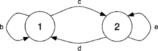
Example 6.12 Let us first write equation (6.31) for the case n = 2:

(6.32)

with f = b + ce*d. Then, consider the automaton of Figure 6.8. M*(1, 1) = f* represents all possible strings that bring the automaton from state 1 back into state 1, i.e. we may either go directly to 1 using b, or change to state 2 with symbol c, then repeat symbol e an arbitrary number of times, which is expressed by e*, and finally return to state 1 with symbol d. This whole procedure can also be repeated indefinitely which altogether gives (b + ce*d)* = f* = M*(1, 1). The other components of M* are interpreted in a similar manner.

The following property of matrices over Kleene algebras will later be useful:

Lemma 6.15 Assume

Then, it holds that B = B + CE*D or equivalently that CE*D ≤ B.

Proof: From (KP5) follows that M* = M** and therefore B = (B + CE*D)* by equation (6.31). Using (SP3) and (KP2) we then have B ≤ B + CE*D ≤ (B + CE*D)* = B and therefore B = B + CE*D.

The proof of this lemma is based on a particular property of Kleene algebras that henceforth becomes important. Namely, that the star operation satisfies the three axioms of a closure operator (Davey & Priestley, 1990). It is therefore common to refer to a* as the closure of a A. In terms of Kleene algebras, the properties of a closure operator are:

They follow directly from (KP2), (KP5) and (KP6). Subsequently, we are going to derive a new generic construction where each valuation corresponds to the closure of a matrix with values from a Kleene algebra. This generates a whole family of new valuation algebras called Kleene valuation algebras. The principal idea behind this construction is motivated from graph related applications as for example from the shortest distance problem. Here, it is obvious that the adjacency matrices of multiple graphs may share the same matrix closure, i.e. different graphs defined over the same set of vertices may have the same shortest distances. Let us explore this observation in more detail by reconsidering square, labeled matrices. Thus, let r be a set of variables, A, +, x, *, 0, 1 a Kleene algebra, M1 M(A, s) and M2 M(A, t) with s, t r. It is then easy to show that the following relation is an equivalence relation between labeled matrices:

(6.33)

This equivalence relation decomposes the set of labeled matrices into disjoint equivalence classes of matrices with equal domains and closures. Moreover, since each closure belongs itself to a different equivalence class, they can be considered as representatives of their associated classes. Thus, defining closures as valuations allows us to compute with a unique representation of graph related knowledge or information.

Let us next introduce some operations to manipulate labeled matrices: For a Kleene algebra the direct sum of M1 M(A, s) and M2 M(A, t) with and is defined as

(6.34)

This operation satisfies the distributive law with respect to the closure operation:

Lemma 6.16 It holds that

Proof: Let O1 M(A, s × t) and O2 M(A, t × s) be two zero matrices for the domains s × t and t × s. Applying equation (6.31) gives

Next, we reconsider the usual projection operator for labeled matrices, but since we only deal with square matrices, we introduce the following shorthand notation:

For M M(A, s) and t ⊆ s we define

(6.35)

However, in the context of Kleene valuation algebras, we need to redefine the operation of vacuous extension for labeled matrices. Instead of assigning the zero element of the semiring to all the new components, we assign the unit element to the diagonal elements and the zero element to all other components. Using the direct sum of matrices, this operation can be defined as follows: For M M(A, s) and s ⊆ t

(6.36)

where is the unit matrix for the domain t - s. The following lemma states that the application of the closure operation and vacuous extension are interchangeable.

Lemma 6.17 For M M(A, s) and s ⊆ t we have

Proof: Due to Lemma 6.16 and (KP3), which implies I = I*, we have

6.7 KLEENE VALUATION ALGEBRAS

We are going to show in this section that closures of labeled matrices over a Kleene algebra A, +, x, *, 0, 1 satisfy the axioms of a valuation algebra. For a countable set of variables r and its lattice of finite subsets D we first define the set of matrix closures as

(6.37)

Under the instantiation of closure matrices as shortest distances in a graph, the operation of projection simply corresponds to dropping distances. On the other hand, vacuous extension corresponds to adding new graph nodes which cannot be accessed from other nodes. It is therefore clear that both operations do not affect other distances. This observation is generalized by the following two lemmas.

Lemma 6.18 is closed under projection.

Proof: We show that for and it holds that

First, observe that it is always possible to decompose M* such that

where and . We then have and therefore

We conclude from (KP2) that E ≤ E*. But using (KP5) and (6.31) we also obtain

which implies E* ≤ E according to (SP3) of Lemma 5.2. This proves that E = E*.

Lemma 6.19 is closed under vacuous extension.

Proof: This follows from Lemma 6.17 and (KP5):

We next introduce a very intuitive combination rule for elements in . Imagine, for example, that we have two closure matrices which express the shortest distances between two possibly overlapping regions of a large graph. Then, the shortest distance matrix for the unified region can be found by vacuously extending the two matrices to their union domain, taking the component-wise minimum which corresponds to semiring addition and computing the new shortest distances. Thus, for M1*, M2* with d(M1*) = s and d(M2*) = t we define

(6.38)

We directly conclude from this definition that is also closed under combination. Moreover, becomes a commutative semigroup as shown by the following lemma.

Lemma 6.20 Combination in is commutative and associative.

Proof: Commutativity of combination follows directly from the commutativity of addition in a semiring. To prove associativity, assume with and . Using Lemma 6.17 we obtain:

The last equality follows from Lemma 6.11 and the associativity of addition. Exactly the same expression can be derived in a similar way for which proves associativity.

Next, we verify the combination axiom:

Lemma 6.21 If and we have

(6.39)

Proof: From the definition of vacuous extension, it follows directly that vacuous extension can be performed step-wise. We therefore obtain

where I is the unit matrix with domain t - z. On the other hand, we also observe that since

Since is closed under vacuous extension, we may apply Lemma 6.15 and obtain

We next compute

This follows from (KP1) and because is closed under projection. We next determine the closure of this matrix using (6.31) and project the result to the domain z:

All these properties imply the following theorem if D denotes the lattice of finite subsets of the countable set r of variables:

Theorem 6.6 The system with labeling, projection (6.35) and combination (6.38) as defined above satisfies the axioms of a valuation algebra.

Proof: Axioms (A2) to (A4) and (A6) follow directly from the above definitions. Axiom (A1) is proved in Lemma 6.20 and Axiom (A5) in Lemma 6.21.

Closures of labeled matrices with values from a Kleene algebra therefore provide another example of a generic construction that leads to as many new valuation algebra instances as Kleene algebras exist. How exactly Kleene valuation algebras are used to solve path problems will be discussed in Section 9.3.3 where we also compare this approach with the solution of factorized path problems using the quasi-regular valuation algebras from Section 6.4. Remember, one reason that motivated the introduction of Kleene valuation algebras was the promise that they always produce idempotent valuation algebras. This and other properties will next be studied.

6.8 PROPERTIES OF KLEENE VALUATION ALGEBRAS

Kleene algebras have many interesting properties as we have seen in Section 6.6. It is therefore not astonishing that Kleene valuation algebras are also very rich in structure. In fact, the following results show that Kleene valuation algebras are idempotent and always provide neutral elements.

Lemma 6.22 Kleene valuation algebras have neutral elements and are stable.

Proof: We first show that the neutral element for the domain s D is given by the identity matrix . Due to Property (KP3) we have I* = I and therefore I . Further, we obtain for M* with d(M*) = s

due to (KP1) and (KP5). It is furthermore clear that projecting a neutral element always results in a neutral element for the subdomain which proves stability.

Lemma 6.23 Kleene valuation algebras are idempotent.

Proof: For M* with we have

This follows from the idempotency of addition, (KP1) and (KP5).

However, Kleene valuation algebras generally do not have null elements. Even if we assume an element for each domain that behaves absorbingly with respect to combination, the nullity axiom of Section 3.4 will not be satisfied. Since projection only drops matrix rows and columns, there may always exist other valuations that project to null elements which contradicts the nullity axiom.

6.9 FURTHER PATH PROBLEMS

This chapter presented two different families of formalisms to model path problems that both satisfy the valuation algebra axioms. Namely, these are quasi-regular valuation algebras and Kleene valuation algebras. Also, it was shown that Kleene valuation algebras provide more algebraic structure as for example the property of idempotency that is not fulfilled in quasi-regular valuation algebras. Looking at the proof of Lemma 6.23, we immediately see that idempotency of combination is a consequence of idem-potent addition and the monotonicity laws in a Kleene algebra. Both requirements are not present in a quasi-regular semiring. On the other hand, the absence of these properties makes quasi-regular semirings more general than Kleene algebras, and the same holds for their induced valuation algebras. Since all path problems shown at the beginning of this chapter are based on Kleene algebras, we end with a few more examples based on only quasi-regular semirings. These applications can therefore not be solved in the formalism of Kleene valuation algebras. The examples are based on the arithmetic semirings of non-negative integers and of real numbers from Example 6.11 that are both quasi-regular but not Kleene algebras. The first instance is a typical graph-related application, whereas the subsequent problems are not directly related to graphs anymore. This keeps the promise articulated in the introduction that the algebraic path problem also covers such rather unexpected applications.

6.6 The Path Counting Problem

Figure 6.9 shows a network similar to the connectivity problem of Instance 6.1. This time however, we ask for the number of paths that connect the source node S with the target node T. We therefore compute the sum of the weights of all possible paths leading from S to T, where the weight of a path corresponds to the product of its edge weights. We compute for the three possible paths:

and then

Clearly, this description corresponds to equation (6.6) based on the arithmetic semiring of non-negative integers.

6.7 Markov Chains

A time-homogeneous, first order Markov chain is specified by a countable sequence of random variables X1, X2, … taking values from a finite state space Ω and satisfying the property:

for all n and . Thus, the probability to arrive in state x at some time depends only on the last state but not on previous states. Such a Markov chain is determined by its transition matrix satisfying

for all X Ω, where the value M(X, Y) specifies the probability to arrive in state Y from the previous state X. A Markov chain can always be represented by a weighted, directed graph where the nodes correspond to the states and the edge weights to the transition probabilities. Let us for example assume a Markov chain with state space Ω = {1, 2, 3} and transition matrix

Its graph is shown in Figure 6.10. For two selected states S and T, the value of the matrix power Mn(S, T) corresponds to the weight of the path between S and T that contains exactly n edges. If the computations are executed in the arithmetic semiring of real numbers , then this path weight corresponds to the probability of reaching state T in n steps from node S. Accordingly, the values of the quasi-inverse matrix M* (S, T) refer to the sum of all probabilities of reaching state T from state S in an arbitrary number of steps. It is clear that this will not be a probability anymore. If we for example obtain M*(S, T) = ∞, we say that the state T has finite hitting time from state S. Moreover, if a state has finite hitting time from itself, then it is called recurrent. Such states return to themselves infinitely often with probability 1. On the other hand, if we obtain a value different from ∞, then the state is called transient and leads back to itself only a finite number of times. Identifying recurrent and transient states in Markov chains is an important task that can thus be seen as an instance of the algebraic path problem. For the above matrix M we obtain by equation (6.17):

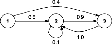
The diagonal values tell us that state 1 is transient and all other states are recurrent. Alternatively, we may repeat these computations with the probabilistic semiring where . This is a Kleene algebra as shown in Example 6.10 and M*(S, T) corresponds to the value of the most likely path from state S to T. We obtain for the above example:

The reader may convince himself that 0.6 · 0.9 = 0.54 is indeed the highest probability among all sequences of transitions that lead from state 1 to state 3. We refer to (Norris, 1998; Meyn & Tweedie, 1993; Kemeny et al., 1960) for a systematic discussion of Markov chains.

6.8 Numeric Partial Differentiation

The numerical computation of the partial derivations of a function can be reduced to an algebraic path problem as shown in (Rote, 1990), from where we also borrow this example. Assume the following function over three variables:

This function is step-wise computed by the following program:

This is a rather simple example but we could as well imagine some complicated program involving loops and conditional statements. However, we next decompose this program into elementary operations:

This decomposition allows us to construct the computational graph of Figure 6.11 by the following procedure: First, a node for is created for each variable Z1 to Z3, Then, we add a node for each elementary operation and connect it with a directed edge to its arguments. If the expression contains a constant, then we first add an additional node for this value.

Now, let us look at some node ω with two outgoing edges leading to u and v. This subtree represents a composition function ω(u, v), whose partial derivatives can be determined by the chain rule:

(6.40)

Note that and can easily be calculated, since only elementary operations are involved. Let us for example take ω = u/v. We then have and . It is therefore possible to assign the weight to each edge (w, v) of the computational graph. We then obtain for the above application of the chain rule:

which is a recursive expression in the unknowns

For the root node r we have . By developing this expression recursively, we obtain the derivative of f with respect to Zi by the sum of the weights of all paths leading from f to Zi, whereas the weight of a path corresponds to the product of its edge weights. So far, we considered the edge weights as symbolic expressions. But if we assign values from the arithmetic semiring of real numbers from Example 6.11 to the variables Z1 to Z3, then all edge weights also correspond to values in this semiring. Then, the above scheme for calculating the partial derivations of f amounts to the solution of a path problem in the quasi-regular semiring of real numbers. Moreover, computing the Jacobi matrix then corresponds to a submatrix of the quasi-inverse matrix that is obtained from solving the all-pairs problem on this setting. We refer to (Rote, 1990) for a more comprehensive analysis of this approach and for related references.

6.9 Matrix Multiplication

Consider a quasi-regular semiring and two square matrices A defined over the same index set. The following idea of reducing the task of multiplying M1 and M2 to the computation of a quasi-inverse matrix was proposed by (Aho et al., 1974). We first construct a new matrix defined as:

We assume the following decomposition of M and compute the quasi-inverse M* by equation (6.17):

Since D and E are zero matrices, we directly obtain F = E + DB*C = O and thus F* = I as a consequence of equation (6.18). We also compute

and finally obtain for the three remaining submatrices:

and B* + B*CF*DB* = B*. This determines the quasi-inverse matrix as

Two square matrices M1 and M2 with equal index sets and values from a quasi-regular semiring can thus be multiplied by computing the quasi-inverse matrix of M and extracting the corresponding submatrix.

6.10 CONCLUSION

This chapter started with an introduction to the algebraic path problem which requires to solve a particular fixpoint equation of matrices taking values from a semiring. In the general case, such equations do not necessarily have a solution, but if they exist, solutions are called quasi-inverses. In order to avoid the problem of non-existence, we limited ourselves to so-called quasi-regular semirings where at least one quasi-inverse exists for each semiring element. Based on the construction of (Lehmann, 1976) it is then possible to compute a particular quasi-inverse of a matrix from the quasi-inverses of the underlying semiring. This leads to a first generic construction called quasi-regular valuation algebra where valuations correspond to labeled pairs of matrices and vectors over a quasi-regular semiring. Such valuation algebras can be used for the solution of the single-target algebraic path problem which will be discussed in Section 9.3.2. A second approach focussing directly on the solution of the all-pairs algebraic path problem is based on a special family of quasi-regular semirings called Kleene algebras. Under this setting, we always obtain the least quasi-inverse for each semiring element and the corresponding operation further satisfies the axioms of a closure operator. These two properties lead to another family of valuation algebras where valuations are closures of labeled matrices over a Kleene algebra. Projection corresponds to simple matrix restriction and combination to the computation of the closure after taking the sum of the two factor matrices. In contrast to quasi-regular valuation algebras, the second approach therefore moves the computational effort from the projection operation to the combination which manifests itself in the fact that Kleene valuation algebras are always idempotent. This combination essentially consists in the computation of a quasi-inverse matrix which, according to (Lehmann, 1976), is possible in polynomial time. Algorithms for this task will be presented in Chapter 9 where we also describe the solution of factorized path problems using quasi-regular and Kleene valuation algebras. Further, we observe that both approaches only store matrices and vectors which also implies that space complexity is polynomial. We therefore have two generic constructions that both induce valuation algebras with a pure polynomial behaviour.

PROBLEM SETS AND EXERCISES

F.1 * Instance 6.5 describes the task of determining the language that brings an automaton from state S to state T as a path problem over the semiring of formal languages from Example 5.7. Alternatively, this can also be interpreted as the problem of listing all paths between node S and node T in a graph, provided that the edge weights express the identifier of the corresponding connection. However, the set of all possible paths between two nodes is often infinite. Thus, we are rather interested in listing only simple paths that contain every edge at most once. Identify the corresponding subsemiring of the semiring of formal languages and determine whether it is still a Kleene algebra.

F.2 * Testing whether a graph is bipartite: An undirected graph is bipartite, if it contains no cycle with an odd number of edges. Since cycles are special paths, we can formulate this as a path problem. Consider the set of symbols A = . The weight of a path is either E, if it contains an even number of edges, or O, if it contains an odd number of edges. Accordingly, the weight of a set of paths is either , E, O or EO, depending on whether the set is empty, contains only even paths, only odd paths or both types of paths. Continue the development of this path problem by specifying how the edge weights are initialized and how the semiring operations are defined. Prove that the semiring is quasi-regular and test if it is also a Kleene algebra. The solution can be found in Section 6.7.1 of (Rote, 1990).

F.3 * Identifying cut nodes of a graph: A cut node in a connected graph is a node whose removal causes the graph to become disconnected. Formulate the problem of finding cut nodes as a path problem and analyze the underlying semiring. The solution can be found in Section 6.7.2 of (Rote, 1990).

F.4 * Prove the following property of Kleene algebras: For a, b A we have

(6.41)

The solution to this exercise is given in Corollary 5 of (Kozen, 1994). Then, prove Lemma 6.14 by applying this identity and the properties of Kleene algebras listed in Section 6.6. The solution to this exercise is given in Chapter 3 of (Conway, 1971).

F.5 * We have seen in Section 3.1 that in case of valuation algebras defined over variable systems, the operation of projection can be replaced by variable elimination. We may then use the simpler versions of the valuation algebra axioms given in Lemma 3.1. Develop the quasi-regular and Kleene valuation algebra from Section 6.4 with variable elimination instead of projection.

F.6 ** It is sometimes necessary to solve many path problems with different Kleene algebras over the same graph. Instead of repeating the computations each time from scratch, we propose a two-stage compilation process: We first determine some formal expression for the paths between S and T which can later be evaluated for different Kleene algebras without recomputing the paths. To define this formal language, we assume a symbol , if an edge between node X and Y exists. In addition, we identify the two semiring operations + and × with the symbols and . Then, the formal expression for the path between node S and T in Figure 6.1 is

This string can now be evaluated by replacing the symbols with concrete edge values and operations from a Kleene algebra.