CHAPTER 7

Ham Antenna Primer

Ham radio antennas fall into two categories: receiving types and transmitting types. Nearly all transmitting antennas can receive signals effectively within the design frequency range. Some, but not all, receiving antennas can transmit signals with reasonable efficiency.

 

Radiation Resistance

When RF current flows in an electrical conductor, such as a wire or a length of metal tubing, some EM energy radiates into space. Imagine that you connect a transmitter to an antenna and test the whole system. Then you replace the antenna with a resistance/capacitance (RC) or resistance/inductance (RL) circuit and adjust the component values until the transmitter behaves exactly as it did when connected to the real antenna. For any antenna operating at a specific frequency, there exists a unique resistance R_R, in ohms, for which you can make a transmitter “think” that an RC or RL circuit is, in fact, that antenna. Engineers call R_R the radiation resistance of the antenna.

Determining Factors

Suppose that you place a thin, straight, lossless vertical wire over flat, horizontal, perfectly conducting ground with no other objects in the vicinity, and feed the wire with RF energy at the bottom. In this situation, the radiation resistance R_R of the wire is a function of its height in wavelengths. If you graph the function, you’ll get Fig. 7-1A.

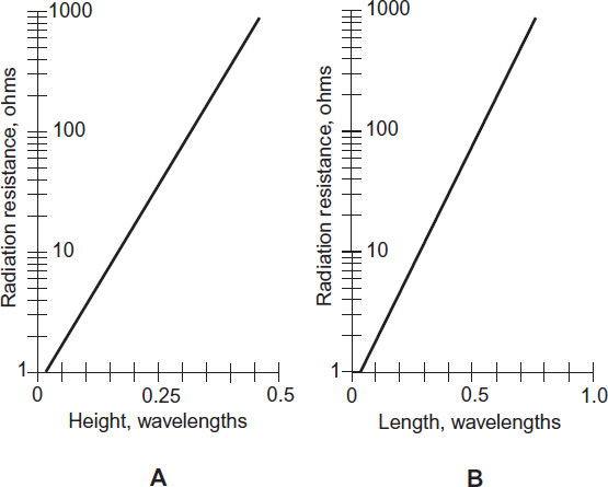
FIGURE 7-1 Approximate values of radiation resistance for vertical antennas over perfectly conducting ground (A) and for center-fed antennas in free space (B).

Now imagine that you string up a thin, straight, lossless wire in free space (such as a vacuum with no other objects anywhere nearby) and feed it with RF energy at the center. In this case, R_R is a function of the overall conductor length in wavelengths. If you graph the function, you’ll get Fig. 7-1B.

Antenna Efficiency

You rarely have to think about antenna efficiency in a receiving system, but in a transmitting-antenna system, efficiency rises to paramount importance! The efficiency expresses the extent to which a transmitting antenna converts the applied RF energy to actual radiated EM energy. In an antenna, radiation resistance R_R appears in series with a certain loss resistance (R_L), and these resistances behave just like any other types of resistors in series: The larger resistance gets more of the energy than the smaller one does.

In an antenna system, loss resistance “gobbles up” the energy and turns it into useless heat, while radiation resistance puts the energy into the airwaves as your transmitted signal. You can calculate the antenna efficiency, Eff, as a ratio with the formula

Eff = R_R / (R_R + R_L)

If you want to get a percentage figure, the expression becomes

Eff_% = 100 R_R / (R_R + R_L)

You can obtain high efficiency in a transmitting antenna only when the radiation resistance greatly exceeds the loss resistance. In that case, most of the applied RF power “goes into” useful EM radiation, and relatively little power gets wasted as heat in the earth and in objects surrounding the antenna.

When the radiation resistance is comparable to, or smaller than, the loss resistance, a transmitting antenna behaves in an inefficient manner. This situation often exists for extremely short antenna radiators because they exhibit low radiation resistance. If you want reasonable efficiency in an antenna with a low R_R value, you must do everything you can to minimize R_L. Even the most concerted efforts rarely reduce R_L to less than a few ohms.

 

Half-Wave Antennas

You can calculate the physical span of an EM field’s half wavelength in free space using the formula

L_m = 150/f_o

where L_m represents the straight-line distance in meters, and f_o represents the frequency in megahertz.

Velocity Factor

The foregoing formula represents a theoretical ideal, assuming infinitely thin conductors that have no resistance at any EM frequency. Obviously, such antenna conductors do not exist in physical reality. The atomic characteristics of wire or metal tubing cause EM fields to travel along a real-world conductor a little more slowly than light propagates through free space. For ordinary wire, you must incorporate a velocity factor, v, of 0.95 (95%) to account for this effect. For tubing or large-diameter wire, v can range down to about 0.90 (90%).

Open Dipole

An open dipole or doublet comprises a half-wavelength radiator fed at the center, as shown in Fig. 7-2A. Each side or “leg” of the antenna measures a quarter wavelength long from the feed point (where the transmission line joins the antenna) to the end of the conductor. For a straight wire radiator, the length L_m, in meters, at a design frequency f_o, in megahertz, for a center-fed, half-wavelength dipole is approximately

L_m = 143/f_o

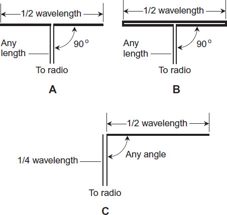
FIGURE 7-2 Basic half-wave antennas. At A, the dipole. At B, the folded dipole. At C, the zepp.

This formula works based on the assumption that v = 0.95, a typical figure for copper wire of reasonable diameter.

In free space, the impedance at the feed point of a center-fed, half-wave, open dipole constitutes a pure resistance of approximately 73 ohms. This resistance represents R_R alone. No reactance exists, because a half-wavelength open dipole exhibits resonance, just as a tuned circuit would if made with a discrete resistor, inductor, and capacitor.

Folded Dipole

A folded dipole antenna consists of a half-wavelength, center-fed antenna constructed of two parallel wires with their ends connected together, as shown in Fig. 7-2B. The feed-point impedance of the folded dipole is a pure resistance of approximately 290 ohms, or four times the feed-point resistance of a half-wave open dipole made from a single wire. This “resistance-multiplication” property makes the folded dipole ideal when using parallel-wire transmission lines.

Half-Wave Vertical

Imagine that you stand a half-wave radiator “on its end” and feed it at the base (the bottom end) against an earth ground, coupling the transmission (feed) line to the antenna through an inductance-capacitance (LC) circuit called an antenna tuner or transmatch, designed to cancel out the reactance and transform the remaining resistance to 50 ohms. Then you connect the other end of the feed line to a radio transmitter. This type of antenna works as an efficient radiator even in the presence of considerable loss resistance R_L in the conductors, the surrounding earth, and nearby objects because the radiation resistance R_R is high.

Zepp

A zeppelin antenna, also called a zepp, comprises a half-wave radiator fed at one end with a quarter-wave section of parallel-wire transmission line, as shown in Fig. 7-2C. The impedance at the feed point is an extremely high, pure resistance. Because of the specific length of the transmission line, the transmitter “sees” a low, pure resistance at the operating frequency. A zeppelin antenna works well at all harmonics (whole-number multiples) of the design frequency. If you use a transmatch to “tune out” reactance, you can use any convenient length of transmission line.

Because of its non-symmetrical geometry, the zepp antenna allows some RF radiation from the feed line as well as from the antenna. That phenomenon sometimes presents a problem in radio transmitting applications. Amateur radio operators have an expression for it: “RF in the shack.” You can minimize woes of this sort by carefully cutting the antenna radiator to a half wavelength at the fundamental frequency, and by using the antenna only at (or extremely near) the fundamental frequency or one of its harmonics.

J Pole

You can orient a zepp antenna vertically, and position the feed line so that it lies in the same line as the radiating element. The resulting antenna, called a J pole, radiates equally well in all horizontal directions. The J pole offers a low-cost alternative to metal-tubing, vertical antennas at frequencies from approximately 10 MHz up through 300 MHz. In effect, the J-pole is a half-wavelength vertical antenna fed with an impedance matching section comprising a quarter-wavelength section of transmission line. The J pole does not require any electrical ground system, a feature that makes it convenient in locations with limited real estate.

 

Quarter-Wave Verticals

The physical span of a quarter wavelength antenna is related to frequency according to the formula

L_m = 75.0v/f_o

where L_m represents a quarter wavelength in meters, f_o represents the frequency in megahertz, and v represents the velocity factor. For a typical wire conductor, v = 0.95 (95%); for metal tubing, v can range down to approximately 0.90 (90%).

You must operate a quarter-wavelength vertical antenna against a low-loss RF ground if you want reasonable efficiency. The feed-point value of R_R over perfectly conducting ground is approximately 37 ohms, half the radiation resistance of a center-fed half-wave open dipole in free space. This figure represents radiation resistance in the absence of reactance, and provides a reasonable impedance match to most coaxial-cable-type transmission lines.

Ground-Mounted Vertical

The simplest vertical antenna comprises a quarter-wavelength radiator mounted at ground level. You feed the radiator at the base with coaxial cable, connecting the cable’s center conductor to the base of the radiator, and the cable’s shield to ground.

Unless you install an extensive ground radial system with a quarter-wave vertical antenna, it will have poor efficiency unless the earth’s surface in the vicinity forms an excellent electrical conductor (salt water, for example). In receiving applications, vertically oriented antennas “pick up” more human-made noise than horizontal antennas do. The EM fields from ground-mounted transmitting antennas are more likely to interfere with nearby electronic devices than are the EM fields from antennas installed high above the ground.

Ground Plane

A ground-plane antenna is a vertical radiator, usually 1/4 wavelength tall, operated against a system of 1/4-wavelength conductors called radials. The feed point, where the transmission line joins the radiator and the hub of the radial system, is elevated. When you place the feed point at least 1/4 wavelength above the earth, you need only three or four radials to obtain low loss resistance for high efficiency. You extend the radials straight out from the feed point at an angle between 0° (horizontal) and 45º below the horizon. Figure 7-3A illustrates a typical ground-plane antenna.

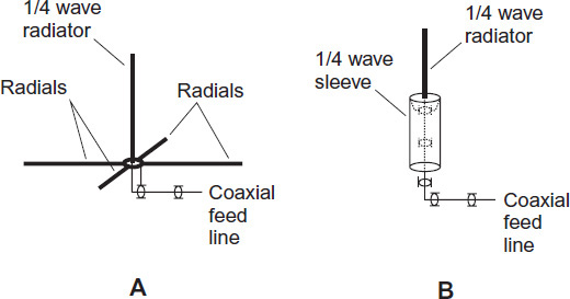
FIGURE 7-3 Basic quarter-wave vertical antennas. At A, the ground-plane design. At B, the coaxial design.

A ground-plane antenna works best when fed with coaxial cable. The feed-point impedance of a ground-plane antenna having a quarter-wavelength radiator is about 37 ohms if the radials are horizontal; the impedance increases as the radials droop, reaching about 50 ohms at a droop angle of 45°. You’ve seen ground-plane antennas if you’ve spent much time around fixed CB-radio installations that operate near 27 MHz, or if you’ve done much ham-radio activity in the VHF bands at 50 or 144 MHz.

Coaxial Antenna

You can extend the radials in a ground-plane antenna straight downward, and then merge them into a quarter-wavelength-long cylinder or sleeve concentric with the coaxial-cable transmission line. You run the feed line inside the radial sleeve, feeding the antenna “through the end,” as shown in Fig. 7-3B. The feed-point radiation resistance equals approximately 73 ohms, the same as that of a half-wave open dipole. This type of antenna is sometimes called a coaxial antenna, a term that arises because of its feed-system geometry, not merely because it’s fed with coaxial cable.

 

Loops

Any receiving or transmitting antenna made up of one or more turns of wire or metal tubing constitutes a loop antenna.

Small Loop

A small loop antenna has a circumference of less than 0.1 wavelength (for each turn) and can function effectively for receiving RF signals. However, because of its reduced physical size, this type of loop exhibits low radiation resistance, a fact that makes RF transmission inefficient unless the conductors have minimal loss. While small transmitting loops exist, you won’t encounter them often because they’re hard to design and expensive to build.

Even if a small loop has many turns of wire and contains an overall conductor length equal to a large fraction of a wavelength or more, the radiation resistance of a practical antenna is a function of its actual circumference in space, not the total length of its conductors. Therefore, for example, if you wind 100 turns of wire around a plastic hoop that’s only 0.1 wavelength in circumference, you’ll end up with a low radiation resistance even though the total length of wire equals 10 full wavelengths!

A small loop exhibits the poorest response to signals coming from along its axis, and the best response to signals arriving in the plane perpendicular to its axis. You can connect a variable capacitor in series or parallel with the loop and adjust it until its capacitance, along with the inherent inductance of the loop, produces resonance at the desired receiving frequency. Figure 7-4 shows an example of a tuned small-loop antenna.

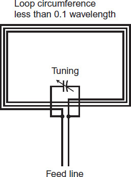
FIGURE 7-4 A small loop antenna with a capacitor for adjusting the resonant frequency.

Hams sometimes use small loops for radio direction finding (RDF) at frequencies up to about 20 MHz, and also for reducing interference caused by human-made noise or strong local signals. A small loop exhibits a sharp, deep null along its axis (perpendicular to the plane in which the conductor lies). When you orient the loop just right, so that the null points in the direction of an offending signal or noise source, the unwanted energy will go way down in strength. In some cases the improvement can exceed 20 dB, meaning that the signal power stays the same, while the offending energy gets 100 times weaker!

Loopstick

For receiving at frequencies up to approximately 20 MHz, a loopstick antenna can function in place of a small loop. This device consists of a coil wound on a solenoidal (rod-shaped), powdered-iron core. A capacitor, in conjunction with the coil, forms a tuned circuit. A loopstick displays directional characteristics similar to those of the small loop antenna shown in Fig. 7-4. The sensitivity is maximum off the sides of the coil (in the plane perpendicular to the coil axis), and a sharp null occurs off the ends (along the coil axis). Loopsticks are often used along with preamplifiers in high-radio-noise environments to enhance reception. Sometimes, a tiny loopstick can “hear” a distant signal even when a large outdoor antenna can’t!

Large Loop

A large loop antenna has a circumference of a half wavelength or a full wavelength (depending on the design), forms a circle, hexagon, or square in space, and lies entirely in a single plane. A well-engineered large loop will work well for transmitting as well as for receiving.

A half-wavelength loop presents a high radiation resistance at the feed point. Maximum radiation/response occurs in the plane of the loop, and a shallow, rather broad null exists along the axis. A full-wavelength loop presents a radiation resistance (and zero reactance, forming a purely resistive impedance) of about 100 ohms at the feed point. The maximum radiation/response occurs along the axis, and minimum radiation/response exists in the plane containing the loop.

The half-wavelength loop exhibits a slight power loss relative to a half-wave open or folded dipole in its favored directions (the physical directions in which it offers the best performance). The full-wavelength loop shows a slight gain over a dipole in its favored directions. These properties hold for loops up to several percentage points larger or smaller than exact half-wavelength or full-wavelength circumferences. Resonance can be obtained by means of a transmatch (antenna tuner) at the feed point, even if the loop itself does not exhibit resonance at the frequency of interest.

 

Ground Systems

End-fed, quarter-wavelength antennas require low-loss RF ground systems to perform efficiently. Center-fed, half-wavelength antennas do not, as they, in effect, provide their own RF grounds. However, good grounding, both for RF and for electrical safety, is advisable for any antenna system to minimize interference and hazards.

Electrical versus RF Ground

Electrical grounding constitutes an important consideration if you plan to have good reception and live for a long time to enjoy it! A good electrical (DC and utility AC) ground can help protect your equipment from damage if lightning strikes in the vicinity. A good electrical ground also minimizes the risk of electromagnetic interference (EMI) to and from radio equipment.

Radio-frequency (RF) grounding is a different “beast” from electrical grounding! You’ll want to have this asset if you want to avoid “RF in the shack” problems, especially if you have an unbalanced antenna system, such as a ground-mounted vertical or an end-fed, random wire. Figure 7-5 shows a proper RF ground scheme (at A) and an improper one (at B). In a good RF ground system, each device goes to a common ground bus, which in turn runs to the earth through a single conductor. This conductor should be as short as you can manage. A poor system has ground loops that act like loop antennas, giving rise to all sorts of havoc.

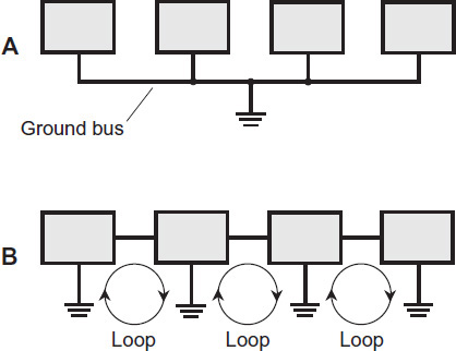
FIGURE 7-5 At A, the correct method for RF grounding of multiple hardware units. At B, an incorrect method for grounding multiple equipments, creating RF ground loops.

Radials and the Counterpoise

A surface-mounted vertical antenna should employ as many grounded radial conductors as possible, and you should make them as long as you can. You can lay the radials right down on the surface, or bury them a few inches (or centimeters) underground. In general, as the number of radials of a given length increases, the overall efficiency of any vertical antenna improves (if all other factors remain constant). Also, as the radial length increases and all other factors remain constant, vertical-antenna efficiency improves. The radials should converge toward, and connect directly to, a ground rod at the feed point, where the transmission line meets the antenna radiator.

A specialized conductor network called a counterpoise can provide an RF ground without a direct earth-ground connection. A grid of wires, a screen, or a metal sheet is placed above the earth’s surface and oriented horizontally to obtain capacitive coupling to the earth’s conductive mass. The feed point of a vertical antenna goes at the center of the counterpoise. This arrangement minimizes RF ground loss, although the counterpoise won’t provide a good electrical ground unless connected to a ground rod driven into the earth, or to the utility system ground.

 

Gain and Directivity

The power gain of a transmitting antenna equals the ratio of the maximum effective radiated power (ERP) to the actual RF power applied at the feed point. Engineers express and measure power gain in decibels (dB). Power gain is usually specified in an antenna’s favored direction(s).

Power Gain Expressions

Suppose that you symbolize the ERP, in watts, for a given antenna as P_ERP, and the applied power, also in watts, as P. Then you can calculate the antenna power gain using the formula

Power Gain (dB) = 10 log₁₀ (P_ERP/P)

In order to define power gain, you must decide upon some sort of reference antenna and define its power gain as 0 dB, meaning no gain or loss at all, in its favored direction(s). A half-wavelength open or folded dipole in free space provides a useful reference antenna for the purpose of comparison with other antennas. Power gain figures taken with respect to a dipole (in its favored directions) are expressed in units called dBd. Some engineers make power-gain measurements relative to a specialized system known as an isotropic antenna, which theoretically radiates and receives equally well in all directions in three dimensions, so it has no favored direction. In this case, units of power gain are called dBi.

For any given antenna, the power gains in dBd and dBi differ by approximately 2.15 dB, with the dBi figure turning out larger:

Power Gain (dBi) = Power Gain (dBd) + 2.15

An isotropic antenna exhibits a loss of 2.15 dB with respect to a half-wave dipole in its favored directions. This fact becomes apparent if you rewrite the above formula as

Power Gain (dBd) = Power Gain (dBi) − 2.15

Directivity Plots

You can portray antenna radiation patterns (for signal transmission) and response patterns (for reception) using graphical plots, such as those in Fig. 7-6. You can assume, in all such plots, that the antenna occupies the center (or origin) of a polar coordinate system. The greater the radiation or reception capability of the antenna in a certain direction, the farther from the center you should plot the corresponding point.

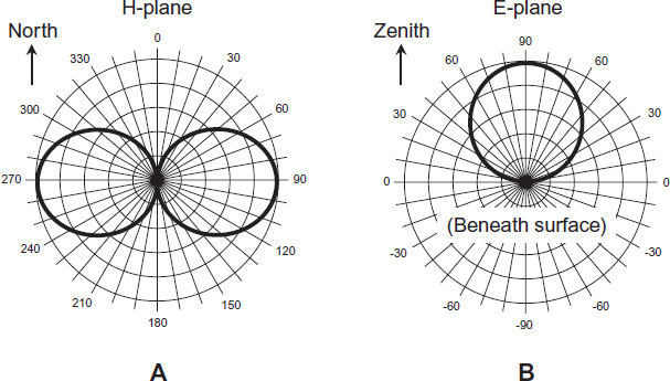
FIGURE 7-6 Directivity plots for a dipole. At A, the H-plane (horizontal plane) plot as viewed from high above the antenna. Coordinate numbers indicate compass direction (azimuth) angles in degrees. At B, the E-plane (elevation plane) plot as viewed from a point on the earth’s surface far from the antenna. Coordinate numbers indicate elevation angles in degrees above or below the plane of the horizon.

A dipole antenna, oriented horizontally so that its conductor runs in a north-south direction, has a horizontal plane (or H-plane) pattern similar to Fig. 7-6A. The elevation plane (or E-plane) pattern depends on the height of the antenna above effective ground at the viewing angle. In most locations, the effective ground comprises an imaginary plane or contoured surface slightly below the actual surface of the earth. With the dipole oriented so that its conductor runs perpendicular to the page or screen (as you look at it in this book or e-reader), and the antenna 1/4 wavelength above effective ground, the E-plane pattern for a half-wave dipole resembles Fig. 7-6B.

Forward Gain

Forward gain is expressed in terms of the ERP in the main lobe (favored direction) of a unidirectional (one-directional) antenna compared with the ERP from a reference antenna, usually a half-wave dipole, in its favored directions. This gain is calculated and defined in dBd. In general, as the wavelength decreases (the frequency gets higher), you’ll find it easier to obtain high forward gain figures.

Front-to-Back Ratio

The front-to-back (f/b) ratio of a unidirectional antenna quantifies the concentration of radiation/response in the center of the main lobe, relative to the direction opposite the center of the main lobe.

Figure 7-7 shows a hypothetical directivity plot for a unidirectional antenna pointed north. The outer circle depicts the RF field strength in the direction of the center of the main lobe, and represents 0 dB (relative to the main lobe, not a dipole). The next smaller circle represents a field strength 5 dB down (a radiation/response level of −5 dB) with respect to the main lobe. Continuing inward, circles represent 10 dB down (−10 dB), 15 dB down (−15 dB), and 20 dB down (−20 dB). The coordinate origin represents 25 dB down (−25 dB) with respect to the main lobe, and also shows the location of the antenna.

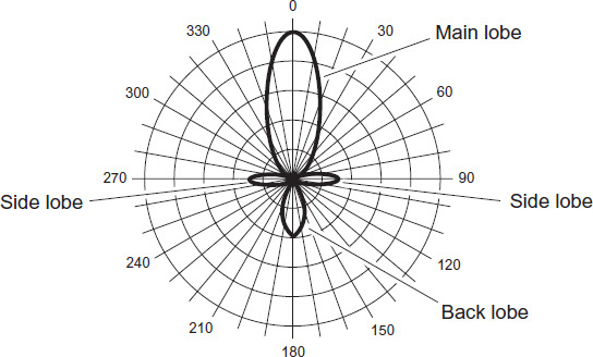
FIGURE 7-7 Directivity plot for a hypothetical antenna in the H (horizontal) plane. You can determine the front-to-back and front-to-side ratios from such a graph. Coordinate numbers indicate compass-bearing angles in degrees.

Front-to-Side Ratio

The front-to-side (f/s) ratio provides another useful expression for the directivity of an antenna system. The specification applies to unidirectional antennas, and also to bidirectional antennas that have two favored directions, one opposite the other in space. You express f/s ratios in decibels (dB), just as you do with f/b ratios. You compare the EM field strength in the favored direction with the field strength at right angles to the favored direction.

Figure 7-7 shows an example. In this situation, you can define two separate f/s ratios: one by comparing the signal level between north and east (the right-hand f/s ratio), and the other by comparing the signal level between north and west (the left-hand f/s ratio). In most directional antenna systems, the right-hand and left-hand f/s ratios theoretically equal each other. However, they sometimes differ in practice because of physical imperfections in the antenna structure, and also because of the effects of conducting objects or an irregular earth surface near the antenna.

 

Phased Arrays

A phased antenna array uses two or more driven elements (radiators connected directly to the feed line) to produce power gain in some directions at the expense of other directions.

End-Fire Array

A typical end-fire array consists of two parallel half-wave open dipoles fed 90° out of phase and spaced 1/4 wavelength apart, as shown in Fig. 7-8A. This geometry produces a unidirectional radiation pattern. Alternatively, the two elements can be driven in phase and spaced at a separation of one full wavelength, as shown in Fig. 7-8B, producing a bidirectional radiation pattern. When you design a phasing system (also called the phasing harness) in any antenna array, you must cut the branches of the transmission line to precisely the correct lengths, taking the velocity factor of the line into account.

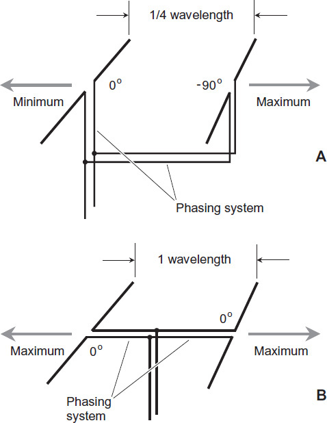
FIGURE 7-8 At A, a unidirectional end-fire antenna array. At B, a bidirectional end-fire array.

Longwire

A wire antenna, measuring a full wavelength or more and fed at a high-current point (current loop) or at one end, constitutes a longwire antenna. A longwire antenna offers gain over a half-wave dipole in certain directions. As you increase the length of the wire, making sure that it runs along a straight line for its entire length, the main lobes get more and more nearly in line with the antenna, and their magnitudes increase. The power gain in the main lobes of a straight longwire depends on the overall length of the antenna: the longer the wire, the greater the gain.

You can consider a longwire as a sort of phased array because it contains multiple points along its span where the RF current attains maximum values. Each of these current loops acts like the center of a half-wave antenna, so the whole longwire in effect constitutes a set of two or more half-wave elements placed end-to-end, with each section phased in opposition relative to the adjacent section or sections. As a result, when you have a wire several wavelengths long, you get a complex radiation pattern; as the length grows, so does the complexity!

Broadside Array

Figure 7-9 shows the geometric arrangement of a broadside array. Each of the driven elements can comprise a single radiator as shown here, or they can consist of more complex antennas with directive properties. In this case, all the driven elements are identical, and are spaced at half-wavelength intervals along the phasing harness, which is a parallel-wire transmission line with a half-twist between each element to ensure that all the elements operate in phase coincidence (exactly the same phase).

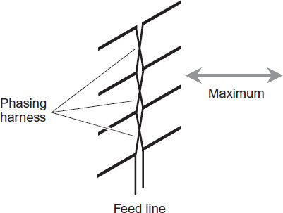
FIGURE 7-9 A broadside array. The elements all receive their portions of the outgoing signal in phase and at equal amplitudes.

The directional properties of any broadside array depend on the number of elements (whether or not the elements have gain themselves), the spacing among the elements, and whether or not a reflecting screen is employed. In general, as you increase the number of elements, the forward gain, the f/b ratio, and the f/s ratios all increase.

 

Parasitic Arrays

Communications engineers and radio hams use parasitic arrays at frequencies ranging from approximately 5 MHz into the microwave range for obtaining directivity and forward gain. Examples include the Yagi antenna and the quad antenna. In the context of an antenna array, the term parasitic describes the characteristics of certain antenna elements. It has nothing to do with parasitic oscillation, a phenomenon that can take place in malfunctioning RF power amplifiers.

Concept

A parasitic element is an electrical conductor that forms part of an antenna system but is not connected directly to the feed line. Parasitic elements operate by means of EM coupling to the driven element or elements. When power gain occurs in the direction of the parasitic element, you call that element a director. When power gain occurs in the direction opposite the parasitic element, you call that element a reflector. Directors normally measure a few percentage points shorter than the driven element(s). Reflectors typically measure a few percentage points longer than the driven element(s).

Yagi

A Yagi antenna, which radio hams sometimes call a beam antenna or simply a beam, comprises an array of parallel, straight antenna elements, with at least one element acting in a parasitic capacity. (The term Yagi comes from the name of one of the original design engineers.)

You can construct a two-element Yagi by placing a director or reflector parallel to, and at a specific distance away from, a single half-wave driven element. The optimum spacing between the elements of a driven-element/director Yagi is 0.1 to 0.2 wavelength, with the director tuned 5% to 10% higher than the resonant frequency of the driven element. The optimum spacing between the elements of a driven-element/reflector Yagi is 0.15 to 0.2 wavelength, with the reflector tuned 5% to 10% percent lower than the resonant frequency of the driven element. Either of these designs gives you a two-element Yagi. The power gain of a well-designed, two-element Yagi in its single favored direction is approximately 5 dBd.

A Yagi with one director and one reflector, along with the driven element, forms a three-element Yagi. This design scheme increases the gain and f/b ratio compared with a two-element Yagi. A well-designed, three-element Yagi exhibits about a 7-dBd gain in its favored direction. Figure 7-10 offers a generic example of the relative dimensions of a three-element Yagi. Although this illustration can serve as a crude “drawing-board” engineering blueprint, the optimum dimensions of a three-element Yagi in practice will vary slightly from the figures shown here, because of imperfections in real-world hardware, and also because of conducting objects or terrain irregularities near the system.

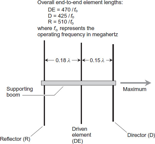
FIGURE 7-10 A three-element Yagi antenna. See text for discussion of specific dimensions. The lowercase, italic Greek lambda (l) means “wavelength.”

The gain, f/b ratio, and f/s ratios of an optimized Yagi all increase as you add elements to the array. You can obtain four-element, five-element, or larger Yagis by placing extra directors in front of a three-element Yagi. When multiple directors exist, each one should be cut slightly shorter than its predecessor.

Quad

A quad antenna operates according to the same principles as the Yagi, except that full-wavelength loops replace the half-wavelength elements.

A two-element quad can consist of a driven element and a reflector, or it can have a driven element and a director. A three-element quad has one driven element, one director, and one reflector. The director has a perimeter of 0.95 to 0.97 wavelength, the driven element has a perimeter of exactly 1 wavelength, and the reflector has a perimeter of 1.03 to 1.05 wavelengths. These figures represent electrical dimensions (taking the velocity factor of wire or tubing into account), not free-space dimensions.

Additional directors can be added to the basic three-element quad design to form quads having any desired numbers of elements. The gain increases as the number of elements increases. Each succeeding director is slightly shorter than its predecessor. Long quad antennas are practical at frequencies above 100 MHz. At frequencies below approximately 10 MHz, quad antennas become physically large and unwieldy, although some ambitious (and daring) hams have constructed quads to work at frequencies down to 3.5 MHz.

 

Antennas for UHF and Microwave Frequencies

At frequencies above 300 MHz (wavelengths less than 1 meter), high-gain, multielement antennas have reasonable physical dimensions and mass because the wavelengths are short.

Horn

A horn antenna looks like a squared-off trumpet. It provides unidirectional radiation and response, with the favored direction coincident with the opening of the horn. The feed line is a waveguide that meets the antenna at the narrowest point (throat) of the horn. (You’ll read more about waveguides later in this chapter.)

Horns are sometimes used all by themselves, but they can also feed large dish antennas at UHF and microwave frequencies. The horn design optimizes the f/s ratio by minimizing extraneous radiation and response that occur if a dipole is used as the driven element for the dish.

Dish

Most people are familiar with dish antennas because of their widespread use in consumer satellite TV and Internet services. Although the geometry looks simple to the casual observer, a dish antenna must be precisely shaped and aligned if you want it to function as intended. The most efficient dish, especially at the shortest wavelengths, comprises a paraboloidal reflector, so named because it’s a section of a paraboloid (the three-dimensional figure that you get when you rotate a parabola around its axis). However, a spherical reflector, having the shape of a section of a sphere, will work okay in most dish designs.

A dish-antenna feed system consists of a coaxial line or waveguide from the receiver and/or transmitter along with a horn or helical driven element at the focal point of the reflector. Figure 7-11A shows an example of a conventional dish feed. Figure 7-11B shows an alternative scheme known as the Cassegrain dish feed. The term Cassegrain comes from the resemblance of this antenna design to that of a Schmidt-Cassegrain reflector telescope.

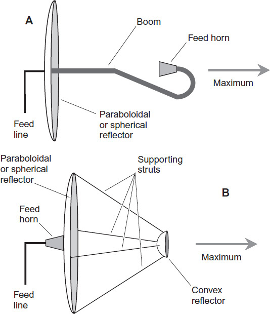
FIGURE 7-11 Dish antennas with conventional feed (A) and Cassegrain feed (B).

As you increase the diameter of the dish reflector in wavelengths, the gain, the f/b ratio, and the f/s ratios all increase, and the width of the main lobe decreases, making the antenna more sharply unidirectional. A dish antenna must measure at least several wavelengths in diameter for proper operation. The reflecting element can consist of sheet metal, a screen, or a wire mesh. If a screen or mesh is used, the spacing between the wires must be a small fraction of a wavelength.

Helical

A helical antenna is a high-gain, unidirectional antenna that transmits and receives EM waves with circular polarization. Figure 7-12 illustrates the construction scheme most often used. The reflector must be at least 0.8 wavelength in diameter at the lowest operating frequency. The radius of the helix should be approximately 0.17 wavelength at the center of the intended operating-frequency range. The longitudinal spacing between helix turns should be approximately 0.25 wavelength in the center of the operating-frequency range. The entire helix should measure at least a full wavelength from end to end at the lowest operating frequency.

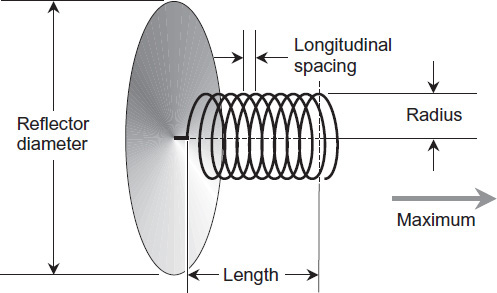
FIGURE 7-12 A helical antenna with a flat reflector.

Corner Reflector

Figure 7-13 illustrates a corner reflector with a half-wave, open-dipole driven element. This design provides some power gain over a half-wave dipole. The reflector is made of wire mesh, screen, or sheet metal. The flare angle of the reflecting element equals approximately 90º. Corner reflectors are widely used in terrestrial communications at UHF and microwave frequencies. For additional gain, several half-wave dipoles can be fed in phase and placed along a common axis with a single, elongated reflector, forming a collinear corner-reflector array.

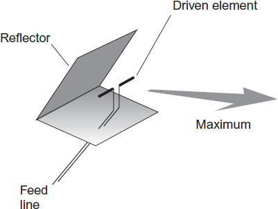
FIGURE 7-13 A corner reflector that employs a dipole antenna as the driven element.

 

Transmission Lines

A transmission line, also known as a feed line, is a medium through which energy gets transferred from one place to another. In ham radio, the expression refers to the line or cable that connects your transmitter and receiver to your antenna.

Characteristic Impedance

The ratio of the signal voltage to the signal current in a transmission line depends on several things. If you connect a noninductive resistor of the correct ohmic value at the far end of a transmission line, where the antenna would normally go, and then you transmit a signal into the line, not exceeding the power dissipation rating of the resistor, the voltage-to-current ratio will remain constant all along the line. This constant ratio will prevail even though the actual voltage and current will decline slightly as you move away from the transmitter (because of line loss, which every transmission line has). The voltage-to-current ratio under these circumstances is called the characteristic impedance or surge impedance of the transmission line. Engineers symbolize it as Z_o.

Coaxial Cable

Coaxial cable is designed for RF signals at frequencies from VLF to UHF. It keeps the desired signals inside itself, and keeps out unwanted signals and interference. Coaxial cable or coax (pronounced “CO-ax”), is used by amateur and CB radio operators to connect transceivers, transmitters, and receivers to antennas. It can also be used in high-fidelity audio systems and computer installations to interconnect components. All coaxial cables are fabricated in the same way: A wire is surrounded by a tube or braid of solid or braided metal. The inner wire is called the center conductor, and the outer conductor is called the shield.

In some coaxial cables, a solid or foamed polyethylene layer, called the dielectric, keeps the center conductor running right down the central axis of the cable, as shown in Fig. 7-14A. The dielectric also keeps the center conductor from shorting out to the shield. Other cables have an uninsulated center conductor and a thin layer of polyethylene just inside the braid (Fig. 7-14B), so that most of the interior of the cable comprises air. In this cable, the center conductor can move around somewhat, but the polyethylene keeps it from shorting out to the shield.

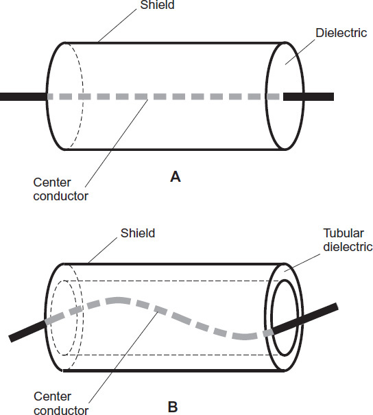
FIGURE 7-14 Coaxial cable with a solid or foamed dielectric (A), and coaxial cable with a dielectric comprising mostly air (B).

In a coaxial cable, the signal is carried by the center conductor. The shield is connected to an electrical ground. Grounding is important for a coaxial cable to function properly. When the shield of the cable is well grounded, it keeps the data signals from “leaking” out of the cable. That’s one of the big advantages of coax. Another advantage is the fact that the shield, when properly grounded, keeps unwanted signals or noise from getting in from sources right next to the cable. Twisted-wire or open-wire lines can let stray RF fields, impulse noise, and appliance noise in, degrading reception.

Parallel-Wire Line

Parallel-wire line is commonly used with balanced (symmetrical) antennas, such as dipoles and most Yagis. The simplest parallel-wire transmission line is open wire. It consists of two wires parallel to each other, with the fewest possible number of intervening supports. The dielectric is almost entirely air. This type of transmission line is one of the oldest, and most effective, ways of getting power from a radio transmitter to an antenna, especially at frequencies below 30 MHz. It’s still used today by many Amateur Radio operators. You can make open-wire line from common electrical wire, such as American Wire Gauge (AWG) No. 12 or No. 14 soft-drawn copper, spaced several inches apart.

The characteristic impedance of an air-dielectric balanced line depends on the radius of the conductors, and also on the spacing between the conductors. If you call the radius of the conductors r and the center-to-center spacing d, as shown in Fig. 7-15A, then you can calculate the approximate characteristic impedance as

Z_o = 276 log₁₀ (d/r)

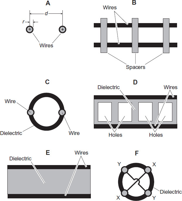
FIGURE 7-15 Open-wire line (A), ladder line (B), tubular line (C), window line (D), ribbon line (E), and four-wire line (F).

as long as you express r and d in the same units, such as centimeters or millimeters. The presence of plastic spacers, employed to keep the conductors evenly separated, will lower this value slightly. Also, if you place the line near objects with a higher dielectric constant than air, the characteristic impedance will go down a little.

Figure 7-15B shows a typical ladder-type, open-wire line. In prefabricated ladder lines, the wires are usually separated by a centimeter or two, and consist of AWG No. 16 or No. 18 soft-drawn uninsulated copper wire. The spacers are placed at regular intervals of about 15 centimeters to keep the wires at constant separation. The characteristic impedance ranges from 300 ohms for a close-spaced ladder line to 450 ohms for the wide-spaced type.

Ladder line has low loss and high power-handling capacity, even in the presence of significant mismatches between the line and the antenna. You’ll usually need an antenna tuner (transmatch) having a balanced output at the station end of the line in shortwave and Amateur Radio installations.

Ladder line works well for residential TV reception using old-fashioned outdoor antennas in fringe areas because this line has lower loss per unit of length, than solid-dielectric lines. Ladder line is also relatively immune to changes in characteristic impedance that can occur when it rains. The main trouble with ladder line is that, if it gets twisted, the conductor spacing will change, and the wires can short out because they lack insulation.

Some of the problems with ladder line and open wire are overcome by so-called tubular line. This type of parallel-wire line can offer performance comparable to ladder line when properly installed and maintained. Figure 7-15C shows an end-on, cross-sectional view of a tubular line. The conductors are molded diametrically opposite each other in a long, flexible cylinder of polyethylene. Tubular lines have Z_o values similar to those of ladder lines. Most of the effective dielectric is air inside the cylindrical supporting structure. This design attribute minimizes line loss per unit of length, and reduces the effects of wetting or icing on the Z_o. To prevent water from collecting inside the tube, you can punch a couple of small holes in the cylinder at physical low points, so that any water that might collect inside the line can run out. One problem with tubular line is the fact that worms, insects, and spiders can get inside the cylinder, lowering the Z_o especially if the creatures spin webs, which hold condensation. This “bugaboo” (pun intended) also lowers the power-handling capacity and increases the line loss. Some tubular lines are hermetically sealed and filled with inert gas to eliminate this trouble, but such lines are expensive, and they cannot be cut if you want to trim the line length.

Parallel-wire line is commonly molded in the edges of polyethylene strips. Some types are suitable for use in Amateur Radio and shortwave-listening stations. This type of line is called twinlead or ribbon. Most twinlead lines have a characteristic impedance of 300 ohms when dry, and when not run near conducting obstructions. You can find this stuff in a variety of forms. Figure 7-15D shows “window” type twinlead. Much of the dielectric is cut away to minimize the line loss, while maintaining constant conductor separation. The “windows” also reduce the extent to which rain affects the characteristic impedance of the line. Figure 7-15E shows twinlead with a solid web of dielectric material. The conductors are stranded copper, usually of size AWG No. 14 to No. 20. Some solid-web types of twinlead have a foamed-polyethylene dielectric for reduced loss. Some hams use TV ribbon in low-power transmitting applications at high frequencies (below 30 MHz) in place of open-wire or ladder line. However, the loss per unit of length of such line exceeds that of open-wire or ladder line. This is attributable to the higher dielectric loss of polyethylene compared with air. Solid-dielectric twinlead is affected considerably by wetness and icing, both of which lower the Z_o and increase the loss even more. In addition, receiving type TV ribbon can’t handle as much power as a good open wire or ladder line can.

Four-wire line is not used as often as other types of parallel-wire line, although it has significant assets. Four conductors are run parallel to each other, in such a way that they form the edges of a long square prism (Fig. 7-15F). Each pair of diagonally opposite conductors is connected together at either end of the line. You can substitute four-wire line for two-wire line in almost any installation. For a given conductor size and spacing, four-wire line has a lower characteristic impedance than two-wire line; the four-wire line is in fact two two-wire lines connected in parallel. It is difficult to construct a two-wire line with a characteristic impedance of less than 150 ohms, but four-wire line can be made to have a Z_o value as low as 75 ohms. Four-wire suffers less than two-wire line from the effects of nearby objects because more of the RF field stays within the line.

Waveguide

A waveguide is an RF transmission line used at UHF and microwave frequencies. In its simplest form, a waveguide consists of a hollow metal pipe having a rectangular or circular cross section. The RF field travels down the pipe, provided that the wavelength is short enough. In order to efficiently propagate RF energy, a rectangular waveguide must have sides measuring at least 0.5 wavelength, and preferably more than 0.7 wavelength. A circular waveguide should measure at least 0.6 wavelength in diameter, and preferably 0.7 wavelength or more. If all of the RF field’s electric lines of flux are perpendicular to the axis of the waveguide, the waveguide is said to operate in the transverse-electric (TE) mode. If all of the magnetic lines of flux are perpendicular to the axis, the waveguide is operating in the transverse-magnetic (TM) mode. In a waveguide, the characteristic impedance varies considerably with the frequency, unlike other types of line in which the Z_o remains independent of the frequency over a wide range. If you plan to use a waveguide, you must keep its interior clean and free from dust or condensation.

Standing Waves

All transmission lines have some loss; they do not transfer energy with perfect efficiency. The loss occurs because of the ohmic resistance of the conductors, because of skin effect (a tendency for RF current to flow mostly near the surface of a conductor), and because of losses in the dielectric. Engineers express this loss in decibels per unit of length. In most lines, the loss per unit of length increases as the frequency goes up. The loss also increases if the load impedance does not match the characteristic impedance of the line.

Standing waves are voltage and current variations that exist on an RF transmission line when the load impedance differs from the Z_o of the line. In a transmission line terminated in a pure resistance having a value equal to the line Z_o, no standing waves occur, and that’s the optimal state of affairs. When standing waves do exist, you’ll get a nonuniform distribution of RF current and RF voltage as you move along the line. As the impedance mismatch between the line and the load (antenna) gets worse, the voltage and current fluctuations, and therefore, the standing waves, grow more pronounced. The ratio of the maximum RF voltage to the minimum RF voltage, or the maximum current to the minimum current, is called the standing-wave ratio (SWR) on the line. The SWR can equal 1:1 only when the current and voltage stay in the same proportions everywhere along the line.

As the mismatch between the line and the load gets worse, the SWR goes up. In theory, there’s no limit to how large the SWR on a transmission line can get. In the extreme cases of a short circuit, open circuit, pure inductance, or pure capacitance at the load end of the line, the SWR is theoretically infinite. In practice, line losses prevent the SWR from becoming truly infinite, but it can reach values of 20:1 or more in a real-world transmission line when a short or open circuit, or a pure reactance (capacitance or inductance), takes the place of the load.

The SWR figure can serve as an indicator of the overall performance of an antenna system because a high SWR indicates a severe mismatch between the antenna and the transmission line. This state of affairs can have an adverse effect on the behavior of a transmitter or receiver connected to the antenna system. An extremely large SWR can also cause significant signal loss in a transmission line. If you connect a high-power transmitter to a transmission line with an extremely high SWR, the currents and voltages can get large enough in some regions of the line to cause physical damage to it. The current can heat the conductors to the point that the polyethylene dielectric material melts; the voltage can cause arcing that melts or burns the dielectric.

 

Stay Safe!

All engineers who work with antenna systems, particularly large arrays or antennas involving the use of long lengths of wire, place themselves in physical peril. By observing some simple safety guidelines, you can minimize (but not completely eliminate) the risk. A few basic tips follow.

     • Never manipulate or install an antenna in such a way that it can fall or blow down on utility power lines. Also, it should not be possible for power lines to fall or blow down on an antenna, even in the event of a violent storm.

     • Never use wireless equipment having outdoor antennas during thundershowers, or when lightning exists anywhere in the vicinity. Antenna construction and maintenance should never be undertaken if you can see lightning or hear thunder, even if a storm appears far away.

     • Disconnect all outdoor antennas from electronic equipment, and connect those antenna feed lines to a substantial earth ground, at all times when you aren’t using your station.

     • Tower and antenna climbing constitutes a job for professionals only. No inexperienced person should ever attempt to climb any antenna support structure. That includes you, most likely. (It certainly includes me!)

     • Indoor transmitting antennas can expose operating personnel to RF field energy. The extent of the hazard, if any, posed by such exposure has not been firmly established. However, sufficient concern exists among some experts to warrant checking the latest publications on the topic. The ARRL can provide you with more information.

Warning! For complete information on antenna safety matters, you should consult a professional antenna engineer or a comprehensive reference devoted to antenna design and construction. You should also read and heed all electrical and building codes for your city, state, or province. Not only will these precautions minimize physical danger to your person and property, but also it will ensure that your “antenna ranch” doesn’t effectively void your homeowner’s insurance policy!