
CHAPTER 1
Hobby Radio: A Technical Overview
Hobby radio encompasses three activities that anyone with a little spare cash and motivation can enjoy: shortwave listening (or SWL), Amateur Radio (also called ham radio), and Citizens Band radio (usually called CB radio). To some extent, they overlap, although ham radio stands above the other two in terms of “fascination potential” (in my opinion). Let’s glance at all three of these hobby radio specialties, and then we’ll review the basics of how radios work. I assume that you already know some electricity and electronics theory, and you’ve picked this book up because you want to take your hobby to new levels. If you need to refresh your memory, I recommend the latest edition of my book Teach Yourself Electricity and Electronics.
Shortwave Radio
Starting over 100 years ago, the radio pioneers called the range of frequencies from 3 to 30 megahertz (abbreviated MHz) the shortwave band. Today, it’s technically called the high-frequency (HF) band. In a latter-day comparative sense, however, both of these expressions constitute misnomers! The waves are long, as they travel through space, compared to the waves in most wireless communications these days. In addition, this band actually represents quite low frequencies in contemporary terms. But the waves are short, and the frequencies are high, compared to the ones used for radio communications and broadcasting when the terms originated.
In the early 1900s, most wireless communication and broadcasting took place at frequencies below 1.5 MHz (wavelengths of more than 200 meters). Engineers and scientists thought that higher frequencies wouldn’t provide good performance in practice, so they all but ignored them as an “electromagnetic wasteland.” The vast region of the radio spectrum comprising wavelengths of “200 meters and down,” corresponding to frequencies of 1.5 MHz and above, remained subject to the whims and ingenuity of Amateur Radio operators and experimenters, who became known as hams because of their flamboyance and supposedly unprofessional character. As things worked out, some hams ended up among the most valuable engineers that the art of communications has ever known.
Within a few years, radio hams discovered that the shortwave frequencies could support long-distance communications and broadcasting on a scale that no one had imagined. In fact, the HF band performed better than the heavily used longer-wavelength frequencies did, allowing reliable contacts spanning thousands of kilometers using transmitters with low or moderate output power. Soon, commercial entities and governments took interest in the shortwave band, and amateurs lost their legal rights to most of it. But hams clung to exclusive operating privileges in small slivers of the shortwave spectrum, thanks in large part to an inventor and ham radio operator named Hiram Maxim, and the HF Amateur Radio bands remain popular to this day.
Shortwave radio still plays a role in international broadcasting, particularly in the developing countries. In technologically advanced nations, most government and business entities have moved their operations to the very high frequencies (VHF) from 30 to 300 MHz, the ultra high frequencies (UHF) from 300 MHz to 3 GHz, and the microwave frequencies above 3 GHz. This ongoing shift has given rise to talk of letting ham radio operators use some additional parts of the shortwave band that they originally discovered.
An HF radio communications receiver, especially one that offers continuous coverage of the spectrum in that general range, is sometimes called a shortwave receiver. Most general-coverage receivers function at all frequencies from 1.5 MHz through 30 MHz. Some also operate in the standard broadcast band at 535 kHz to 1.605 MHz. A few receivers, called allwave receivers, can function below 535 kHz and into the longwave radio band, as well as in bands at frequencies above 30 MHz.
Anyone can build or obtain a shortwave or general-coverage receiver and listen to signals from all around the world. This hobby is called shortwave listening (SWL). Millions of people all over the world enjoy it. In the United States, the proliferation of computers and Internet communications has largely overshadowed SWL since the 1980s, and many young Americans grow up ignorant of a realm of broadcasting and communications that still prevails in much of the world.
Various commercially manufactured shortwave receivers exist on the market, ranging in price from under $100 to thousands of dollars. A simple wire receiving antenna, which is all you need to receive the signals, costs practically nothing. Some of the better electronics or hobby stores carry these receivers, along with antenna equipment, for a complete installation. You can also shop around in consumer electronics and Amateur Radio magazines.
Amateur (Ham) Radio
In most countries, people must obtain government-issued licenses to send messages by means of Amateur Radio. Hundreds of thousands of people have Amateur Radio licenses in the United States. You won’t have trouble getting a ham radio operator’s license if you know electricity and electronics fundamentals. If you want to get started with this hobby, you can contact your local Amateur Radio club or the American Radio Relay League (ARRL) in Newington, Connecticut.
Ham radio operators communicate by talking, sending Morse code, or typing on computers. Typing the text on a computer resembles using the Internet. In fact, some ham radio groups or clubs have set up their own radio networks, and quite a few have “patched” into the Internet as well. Some hams, rather than talking or texting or using Morse code (also called CW for continuous waves, even though the waves are broken up into dots and dashes) on the radio, prefer to experiment with electronic circuits, and sometimes they come up with designs that find their way into commercial and military equipment.
Some hams simply chat about anything that comes to mind (except business matters, which remain illegal to discuss using the ham radio frequencies in the United States). Others like to practice their emergency-communications skills, so that they can serve the public during crises, such as hurricanes, wildfires, earthquakes, or floods. Still others like to venture into the wilderness and talk to people thousands of kilometers away while sitting outdoors under the stars. Radio hams communicate from cars, trucks, trains, boats, aircraft, motorcycles, bicycles, and even on foot.
The simplest ham radio station has a transceiver (transmitter/receiver), a microphone, and an antenna. A modest ham radio station fits easily on a desk, and has a footprint roughly the size of a personal desktop computer, keyboard, and monitor. If you want, you can add accessories until your “rig” takes up an entire room in the house or the better part of a cellar, as does my installation shown in Fig. 1-1. You’ll also need an antenna of some sort, preferably located outdoors. Figure 1-2 shows my vertical antenna designed to operate at 14 MHz, one of the most popular ham radio frequency bands, also called 20 meters (approximately the length of the radio waves at that frequency).
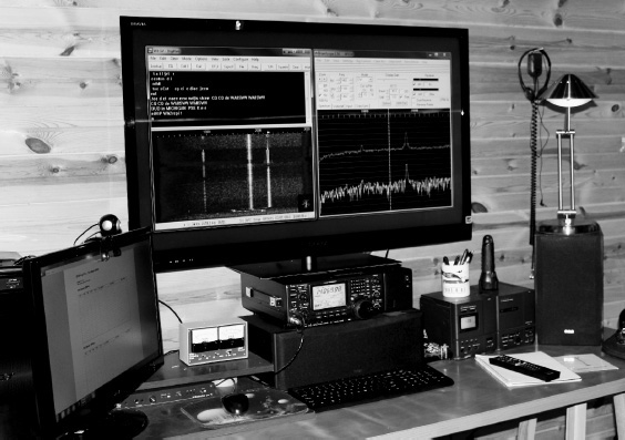
FIGURE 1-1 My ham radio station includes a transceiver, an Internet-ready computer, an interface for digital communications, a power output and antenna testing meter, an audio amplifier with four speakers (one shown here, at extreme right) and two displays, one of which is a 46-inch high-definition television set.
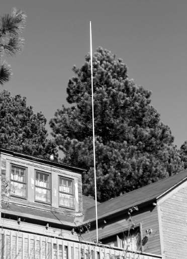
FIGURE 1-2 Here’s a photo of the antenna for the ham radio station shown in Fig. 1-1. It’s made of telescoping sections of aluminum tubing, mounted on a deck railing, and can go up or come down in a couple of minutes to accommodate the rapidly changing weather conditions characteristic of my location.
Figure 1-3 is a block diagram of a typical home ham radio station. The computer can serve to network with other hams who own computers, and it functions as a terminal for the transceivers. If desired, the computer can also control the antennas for the station, and can keep a log of all stations that have been contacted. Most modern transceivers can be remotely operated by computer either over the radio or using the Internet.
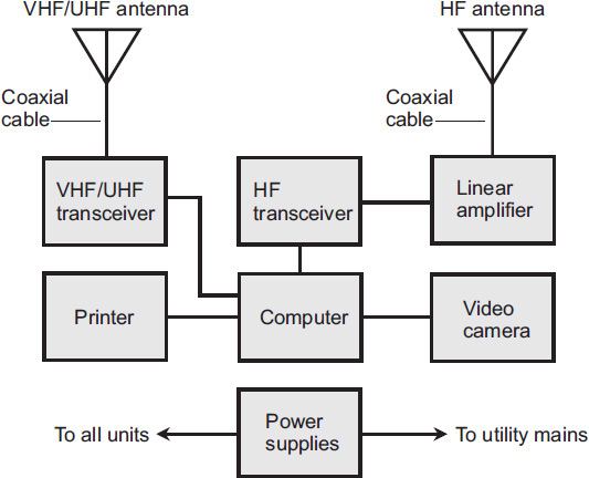
FIGURE 1-3 Block diagram of a well-equipped fixed-location Amateur Radio station. This system has an external linear amplifier (a precision radio transmitting amplifier) for generating high-power signals on some frequencies. Abbreviations: HF = high frequency (3 MHz to 30 MHz); VHF = very high frequency (30 MHz to 300 MHz); UHF = ultra high frequency (300 MHz to 3 GHz).
Figure 1-4 shows a ham radio transceiver for use in a vehicle (upper unit) on the 2-meter band corresponding to frequencies of 144 to 148 MHz. Two-way radio use from any sort of vehicle (car, truck, boat, train, aircraft, or even bicycle) is called mobile operation, and radios especially designed for that application are known as (you guessed it) mobile radios. While mobile operation can give you plenty of fun, you should keep in mind the ever-growing possibility that your state or municipality might outlaw it some day if they haven’t already. In particular, you might not be allowed to use your transmitter while driving the vehicle.
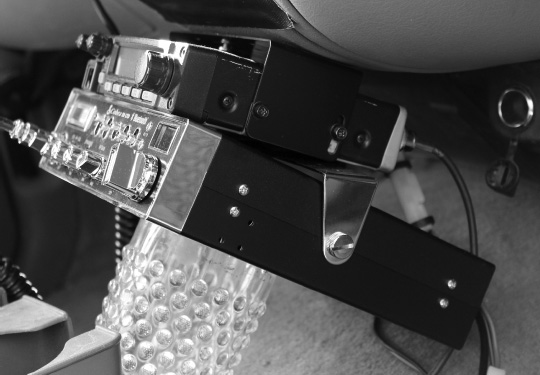
FIGURE 1-4 Two-way radios mounted under the dashboard of my vehicle. An amateur mobile transceiver rests on top, and a CB mobile transceiver sits underneath it. A plastic cup, wedged underneath the CB radio, keeps both units from wobbling.
Warning! Don’t even think about transmitting signals on the Amateur Radio frequencies without getting a license first. If you commit that offense, you can face large fines; in some cases they range in the tens of thousands of dollars. (Yes, the authorities can catch you.) In the United States, several classes of ham radio licenses exist, all of which are issued by the Federal Communications Commission (FCC). For complete information, contact the headquarters of the ARRL at 225 Main Street, Newington, CT 06111 or on the Web at
The ARRL publishes excellent books that deal with all subjects relevant to ham radio, as well as up-to-date license exam study materials. The people at ARRL headquarters can tell you the locations of some Amateur Radio clubs near you, where you can meet hams of all “stripes.”
Citizens Band (CB) Radio
The Citizens Radio Service, also known as Citizens Band (CB), is a radio communications and control service. The most familiar CB mode, called Class D, operates on 40 channels at frequencies around 27 MHz (corresponding to a wavelength of 11 meters).
Normally, the communications range on the 11-meter band rarely exceeds 30 kilometers. However, at times of peak sunspot activity, worldwide communication is possible on this band, a feature that brings both good and bad consequences. While you can have fun listening to people who live thousands of kilometers away on a simple radio unit, those same stations can drown out local ones, perhaps the rancher “next door” with whom you want to discuss business (which is legal on CB radio), or the highway patrol officer whom you are trying to reach when your truck breaks down in some remote place where cell phones won’t work.
The original 11-meter band had 23 channels, and only amplitude modulation (AM) was used. The maximum allowed transmitter power was 5 watts “input to the final amplifier,” corresponding to around 3.5 watts of actual radio-frequency (RF) output power. Unlicensed operation was allowed if the power was 100 milliwatts (0.1 watt) or less. Because of the explosion in CB use during the 1970s, the Federal Communications Commission (FCC) increased the number of channels to 40 in the United States, and single-sideband (SSB) voice mode was introduced to conserve spectrum space and improve communications reliability. The maximum legal power output was set at 12 watts peak. Licensing requirements were done away with.
The Citizens Radio Service has been “spiced up” by so-called pirates and freebanders, who use illegal amplifiers and/or operate outside the legal frequency limits of the band. Freeband activity reaches its peak during times of maximum sunspot numbers when long-distance communication can often take place. Some CB operators, legitimate or otherwise, take a conservative route and obtain Amateur Radio licenses to explore the wider horizons offered by that service. They get exposed to a lot more interesting opportunities than the freebanders do, and they can do it all within the scope of the law!
In emergencies, CB radio can save lives. Motorists, hikers, boaters, and small-aircraft pilots use these radios to call for help when stranded. Small CB radio sets, with reduced-size magnetic-mount antennas, are available for motorists, intended for use in emergencies. Some CB operators, in contrast, enjoy the recreational aspect of radio communication. During the 1970s, CB radio became popular among truckers, and remains so to this day, especially in the American South.
If you drive through truly remote locations where your cell phone won’t work, an HF mobile ham radio set will serve to get you help, even if you have to contact someone hundreds of kilometers away to call the state troopers for you! For these reasons, this book won’t deal any further with CB radio. If you’re a freebander right now, let me recommend that you get a ham radio license and enjoy radio communications to its fullest. Maybe after reading this book you’ll see what I mean!
Electromagnetic Fields
In a radio or television transmitting antenna, electrons move back and forth between the atoms in a metallic wire or tubing. The electrons’ velocity constantly changes as they speed up in one direction, slow down, reverse direction, speed up again, and so on. When electrons move, they generate a magnetic field. When electrons accelerate (change speed), they generate a fluctuating magnetic field. When electrons accelerate back and forth at a defined and constant pace, they generate an alternating magnetic field at the same rate, or frequency, as that of their motion.
An alternating magnetic field gives rise to an alternating electric field, which in turn spawns another alternating magnetic field, and then another electric field, and so on indefinitely. As this occurs, you get a so-called electromagnetic (EM) field that can travel through space over vast distances, perpendicular to the electric and magnetic “lines of force,” and outward from the energy source (such as your antenna) at the speed of light, approximately 300,000 kilometers per second.
All EM fields have two important properties: the frequency and the wavelength. When you quantify them, you find that they exhibit an inverse relation: as one increases, the other decreases. You can express EM wavelength as the physical distance between any two adjacent points at which either the electric fields or the magnetic fields have identical strength and orientation.
An EM field can have any conceivable frequency, ranging from years per cycle to trillions of cycles per second (hertz). Our sun has a magnetic field that oscillates with a 22-year cycle. Radio waves oscillate at thousands, millions, or billions of hertz. Infrared, visible light, ultraviolet, X rays, and gamma rays comprise EM fields that alternate at many trillions (million millions) of hertz. The wavelength of an EM field can likewise vary over the widest imaginable range, from quadrillions of kilometers to millionths of a millimeter.
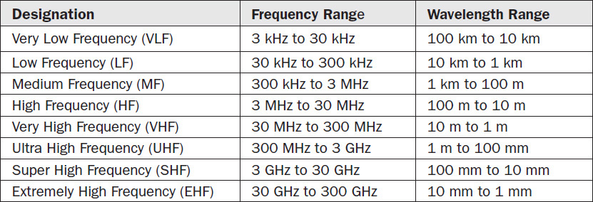
Physicists, astronomers, and engineers refer to the entire range of EM wavelengths as the EM spectrum. Scientists use logarithmic scales to depict the EM spectrum, as shown in Fig. 1-5A, according to the wavelength in meters (m). The radio-frequency (RF) spectrum, which includes radio, television, and microwaves, appears expanded in Fig. 1-5B, where the axis is labeled according to frequency. The RF spectrum breaks down in bands from very low frequency (VLF) through extremely high frequency (EHF), according to the criteria outlined in Table 1-1. As far as I know, engineers and scientists haven’t formally demarcated the exact lower limit of the VLF range; it varies depending on whom you consult. Let’s call it 3 kHz.
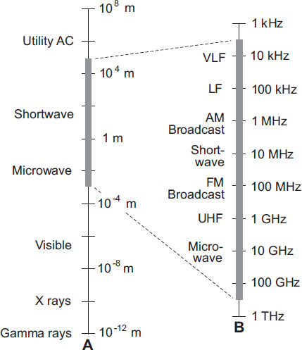
FIGURE 1-5 Drawing A shows a nomograph of the electromagnetic (EM) spectrum at wavelengths ranging from 108 meters (m) down to 10−12 m. Each vertical division represents two orders of magnitude (two powers of 10). At B, you see a nomograph of the radio-frequency (RF) portion of the spectrum, where each vertical division represents one order of magnitude.
TABLE 1-1 Frequency bands in the RF spectrum. Abbreviations: kHz = kilohertz or thousands of hertz; MHz = megahertz or millions of hertz; GHz = gigahertz or billions (thousand-millions) of hertz; m = meters; km = kilometers or thousands of meters; mm = millimeters or thousandths of a meter.
Radio Wave Propagation
The movement of radio waves through space at the speed of light is called wave propagation. This phenomenon has fascinated scientists for well over a century, ever since “electromagnetic pioneers,” such as Heinrich Hertz, Guglielmo Marconi, and Nikola Tesla, discovered that EM fields can travel over long distances without any humanmade infrastructure, such as wires, cables, optical fibers, or satellites. Let’s examine some wave propagation behaviors that affect wireless communications at radio frequencies, and that, if you take up any sort of radio-related hobby, will interest you.
Polarization
You can define the orientation of the electric “lines of force,” technically known as flux lines, as the polarization of an EM wave. If these lines (not real threads or objects of any sort, but theoretical artifacts) run parallel to the earth’s surface, you have horizontal polarization. If the electric flux lines run perpendicular to the earth’s surface, you have vertical polarization. Polarization can also have a “slant” that goes at any angle you can imagine.

Line-of-Sight Waves
Radio waves always travel in straight lines unless something makes them bend, bounce, or turn corners. So-called line-of-sight propagation can take place when the receiving antenna isn’t actually visible from the transmitting antenna because radio waves penetrate nonconducting opaque objects such as trees and frame houses. The line-of-sight wave consists of two components called the direct wave and the reflected wave.
• In the direct wave, the longest wavelengths are least affected by obstructions. At very low, low, and medium frequencies, direct waves can diffract (go around corners in obstructing objects). As the frequency rises, and especially when it gets above 3 MHz or so, obstructions have more blocking effect on direct waves.
• In the reflected wave, the RF energy reflects from the earth’s surface and from conducting objects, such as wires and steel girders. The reflected wave always travels farther than the direct wave. The two waves might arrive at the receiving antenna in perfect phase coincidence so that they reinforce each other, but usually they don’t.
If the direct and reflected waves arrive at the receiving antenna with equal strength but such that one wave lags behind the other by 1/2 cycle, you observe a dead spot. The same effect occurs if the two waves arrive inverted in phase with respect to each other (that is, in phase opposition). The dead-spot phenomenon is most noticeable at the highest frequencies. At VHF and UHF, an improvement in reception can sometimes result from moving the transmitting or receiving antenna only a few centimeters! In mobile operation, when the transmitter and/or receiver move, multiple dead spots produce rapid, repeated interruptions in the received signal, a phenomenon called picket fencing.
Surface Waves
At frequencies below about 10 MHz, the earth’s surface conducts alternating current (AC) quite well, so vertically polarized radio waves can follow the surface for hundreds or even thousands of kilometers, with the earth helping to transmit the signals. As you reduce the frequency and increase the wavelength, you observe decreasing ground loss, and the waves can travel progressively greater distances by means of surface-wave propagation. Horizontally polarized waves don’t travel well in this mode, because the conductive surface of the earth in effect shorts out horizontally oriented electric fields.
Sky Waves
The upper atmosphere, when influenced by ultraviolet radiation and X rays from the sun, can return radio waves to the earth at certain frequencies. This so-called ionosphere has several zones of ionization (regions where the atmosphere’s atoms have an electric charge) that occur at fairly constant, predictable altitudes, as shown in Fig. 1-6.
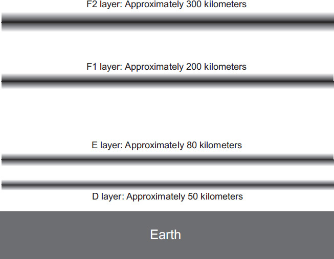
FIGURE 1-6 The ionosphere appears above the earth’s surface at various altitudes in layers called D, E, F1, and F2. The most spectacular long-distance shortwave propagation results from the effects of the uppermost layers.
The lowest ionized region is called the D layer. It forms at an altitude of about 50 kilometers, and ordinarily exists only on the daylight side of the planet. This layer absorbs radio waves at some frequencies, effectively preventing long-distance radio-wave propagation.
The E layer, which forms about 80 kilometers above the surface, exists mainly during the day, although nighttime ionization sometimes occurs. The E layer can provide medium-range radio communication at certain frequencies. Often it forms in “clouds” and can change its character rapidly, hence the origin of the term sporadic-E propagation.
At higher altitudes, you find the F1 layer and the F2 layer. The F1 layer, normally present only on the daylight side of the earth, forms at about 200 kilometers altitude; the F2 layer exists at about 300 kilometers over most, or all, of the earth, on the nighttime side as well as the daylight side. Sometimes, radio enthusiasts ignore the distinction between the F1 and F2 layers, and speak of them together as the F layer.
Tropospheric Propagation
At frequencies above about 30 MHz (wavelengths shorter than about 10 meters), the lower atmosphere bends radio waves towards the surface. Tropospheric bending occurs because the index of refraction of air, with respect to radio waves, decreases with altitude. It’s the same effect that makes sound waves travel for long distances under certain conditions, such as a calm evening on a big lake. Tropospheric bending can allow you to communicate for hundreds of kilometers, even when the ionosphere will not return waves to the earth.
Another tropospheric-propagation mode is called tropospheric scatter or troposcatter. This phenomenon takes place because air molecules, dust grains, and water droplets scatter some of the EM field, just as they scatter light rays. You’ll observe troposcatter most commonly at VHF and UHF. Troposcatter always occurs to some extent, regardless of the weather conditions. Figure 1-7 shows examples of tropospheric bending and scatter effects.
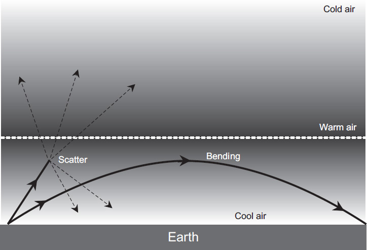
FIGURE 1-7 The earth’s lower atmosphere (the troposphere) can affect radio waves at some frequencies. The most common effects are scattering and bending.
Ducting, a peculiar type of tropospheric propagation, occurs less often than bending or scatter, but offers more dramatic effects. Ducting takes place when EM waves get “trapped” within a layer of cool, dense air between two layers of warmer air, a phenomenon called the duct effect. Like bending, ducting occurs mostly at frequencies above 30 MHz.
Auroral Propagation
When the sun gets unusually active, the Aurora Borealis (“northern lights”) and the Aurora Australis (“southern lights”) can return radio waves to the earth, facilitating auroral propagation. The aurora occur at altitudes of about 60 to 400 kilometers. The effect occurs day and night, even though the “lights” can only be seen visually at night. Theoretically, auroral propagation can occur between any two points on the earth’s surface from which the same part of an active aurora region lies on a line of sight. Auroral propagation seldom occurs in the tropics or subtropics, when either the transmitting station or the receiving station is located at a latitude less than 35° north or south of the equator. It’s most common in and near the Arctic and Antarctic.
Auroral propagation causes rapid and severe signal fading (changes in strength), which renders analog voice and video signals unintelligible. Digital modes work somewhat better, but the signal frequency gets “spread out” or “smeared” over a band several hundred hertz wide as a result of phase modulation induced by auroral motion. This “spectral spreading” limits the maximum data transfer rate. For serious users of this mode, Morse code in the form of simple on/off keying offers by far the best option. Auroral propagation usually takes place along with poor ionospheric propagation resulting from sudden eruptions called solar flares on the sun’s surface, so if normal propagation suddenly deteriorates, you might want to check for aurora effects!
Meteor Scatter Propagation
As meteoroids from space enter the earth’s upper atmosphere to become meteors, they produce ionized trails that persist for a fraction of a second up to several seconds. The exact duration of any given meteor trail depends on the size of the meteor, its speed, and the angle at which it enters the atmosphere. A single trail rarely lasts long enough to allow transmission of much data. However, during a meteor shower, multiple trails can produce almost continuous ionization for a period of hours. Ionized regions of this type can reflect radio waves at certain frequencies. Communications engineers call this effect meteor scatter propagation. It can take place at frequencies far above 30 MHz and over distances of up to about 2400 kilometers.
Moonbounce Propagation
Some radio amateurs, blessed with the cash for an elaborate station and a desire for technical adventure, engage in Earth-moon-earth (EME) communications, also called moonbounce, at VHF and UHF. Successful moonbounce communication requires a sensitive receiver using a specially designed preamplifier, a large directional antenna, and a high-power transmitter. The preferred modes are CW and WSJT.
Signal path loss presents the main difficulty for anyone who contemplates EME communications. Received EME signals are always weak. High-gain directional antennas must remain constantly aimed at the moon, a requirement that dictates the use of steerable antenna arrays, preferably controlled by computers. The EME path loss increases with increasing frequency, but this effect is offset by the more manageable size of high-gain antennas as the wavelength decreases.
Solar noise can pose a problem with moonbounce, as well. Communication becomes most difficult near the time of the new moon, when the moon lies near a line between the earth and the sun because the sun generates strong radio waves (as well as infrared, visible light, ultraviolet, and X rays). Problems can also occur with cosmic noise when the moon passes near “bright” regions in the so-called radio sky. The constellation Sagittarius lies in the direction of the center of the Milky Way galaxy, and EME performance suffers when the moon passes in front of that part of the stellar background because all those stars, like our sun, are gigantic radio noise transmitters!
The moon keeps the same face more or less toward the earth at all times, but some back-and-forth “wobbling” occurs. This motion, called libration (not liberation or libation) produces rapid, deep fluctuations in signal strength, a phenomenon known as libration fading. The fading becomes more pronounced as the operating frequency increases. It occurs as multiple transmitted radio wavefronts reflect from myriad topographical formations, such as craters and mountains on the moon’s surface, whose relative distances constantly change because of the “wobbling.” The reflected waves recombine in constantly shifting phases at the receiving antenna, sometimes reinforcing each other to produce a stronger signal, and at other times canceling to produce a deep fade.
Morse Code and Radioteletype
The Morse code is a binary (two-state) scheme for sending and receiving messages by electronic means, and it’s also the oldest! Engineers call it a binary code because it has only two possible conditions, either “all the way off” or “all the way on.” Historically, English-speaking radio and telegraph operators have used two different Morse codes. Nowadays, the commonly used code is the International Morse Code or Continental Code. In the early days of telegraph, operators used a slightly different code known as the American Morse code.
On/Off Keying
In ham radio Morse code, the elements are sometimes called dots and dashes, where a dot comes over your speaker or headset as a short audio tone and a dash comes through as a longer tone (three times longer, in the ideal case). Speeds are expressed in words per minute (wpm).
The Morse code, when transmitted using simple on/off keying, breaks down into an indefinite sequence of digital intervals or bits (binary digits), where the signal exists during the whole length of the bit, or else for none of it at all. The key-down (audio tone) condition is called mark, and the key-up (silent) condition is called space. The dot comprises a mark condition that lasts for one bit; the dash is a mark that lasts for three bits. The spaces between dots and dashes within a single character are one bit long. The spaces between characters are three bits long, and the spaces between words and after sentences are seven bits long.
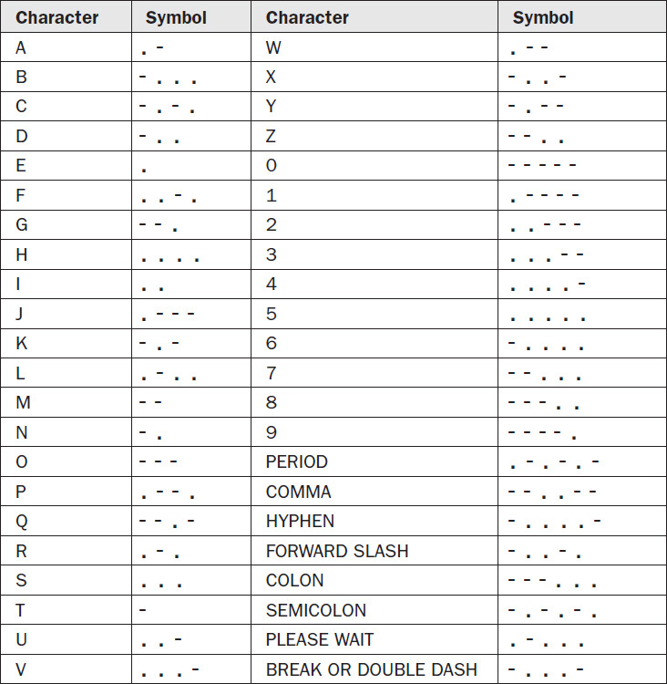
Table 1-2 shows the International Morse Code characters used in the United States and other countries that have the same alphabet as the English language does. The code characters vary in languages that use other written symbols, such as Cyrillic, Greek, Arabic, Hebrew, Chinese, and Japanese.
TABLE 1-2 Symbols in the International Morse Code for English and Other Languages That Use the Same Alphabet
Frequency-Shift Keying
You can send digital data faster, and with fewer errors, than Morse code allows if you use frequency-shift keying (FSK). In FSK systems, the carrier frequency shifts between mark and space conditions, usually by a few hundred hertz or less. The two most common codes that ham radio operators use with FSK are Baudot (pronounced “baw-DOE”) and ASCII (pronounced “ASK-ee”). The acronym ASCII stands for American Standard Code for Information Interchange.
In radioteletype (RTTY) FSK systems, a terminal unit (TU) converts the digital signals into electrical impulses that operate a teleprinter, or display the characters on a computer screen. The TU also generates the signals necessary to send RTTY when an operator types on a keyboard. A device that sends and receives FSK is sometimes called a modem, an acronym that stands for modulator/demodulator.
When conditions aren’t too bad, FSK works better than on/off Morse-code style keying for data communications because the space signals are specifically identified that way (in other words, their existence is confirmed by an actual signal rather than by silence). A sudden noise burst in an on/off keyed signal can “confuse” a receiver into falsely reading a space as a mark when on/off keying is used, but when the space is positively represented by its own signal, this type of error happens far less often.
Voices on Waves
An audio voice signal comprises frequency elements that lie mostly in the range between 300 Hz and 3 kHz. You can modulate some characteristic of a radio wave, also called a radio-frequency (RF) carrier, with an audio voice waveform, thereby transmitting the voice information over the airwaves.
Amplitude Modulation
Figure 1-8 shows a simple bipolar-transistor circuit for obtaining amplitude modulation (AM). You can imagine this circuit as an RF amplifier for the carrier, with the instantaneous gain (moment-to-moment amplification factor) dependent on the instantaneous audio input amplitude.
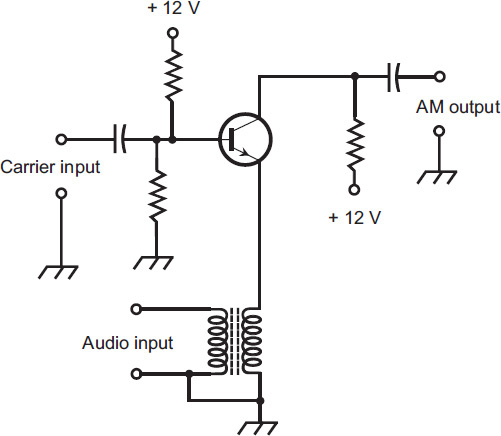
FIGURE 1-8 An amplitude modulator using an NPN bipolar transistor. You can think of this circuit as an amplifier whose gain (amplification factor) depends on the voice input level from instant to instant in time.
The circuit shown in Fig. 1-8 will perform quite well, as long as you don’t let the audio input level get too high. If you inject an audio signal that’s too strong, you’ll end up with distortion (nonlinearity) in the transistor, resulting in degraded intelligibility (understandability), reduced circuit efficiency (ratio of useful power output to total power input), and excessive output signal bandwidth (the difference between the highest and lowest signal frequency).
In an AM signal, you can express the modulation extent as a percentage ranging from 0%, representing an unmodulated carrier, to 100%, representing the maximum possible modulation you can get without introducing distortion into the signal. In an AM signal modulated at 100%, you’ll find that 1/3 of the signal power conveys the voice information, while the carrier wave gobbles up the other 2/3 of the power. That characteristic makes AM a mighty inefficient way to convey information!
Figure 1-9 shows a spectral display of a generic AM voice radio signal at a single instant in time. Frequency appears on the horizontal scale, which runs in increments of 1 kHz per division. Amplitude appears on the vertical scale; each division represents ±3 dB of change in signal strength (a doubling or halving of the signal power). The maximum (reference) amplitude of 0 dB represents 1 milliwatt of power, a condition that engineers abbreviate as 0 dBm (0 decibels relative to 1 milliwatt). In a display of this type, the voice data shows up as sidebands above and below the carrier frequency. These sidebands are the result of sum and difference signals produced by a mixing effect that takes place in the modulator circuit between the audio and the carrier. The RF energy between −3 kHz and the carrier frequency is called the lower sideband (LSB); the RF energy from the carrier frequency to +3 kHz is called the upper sideband (USB).
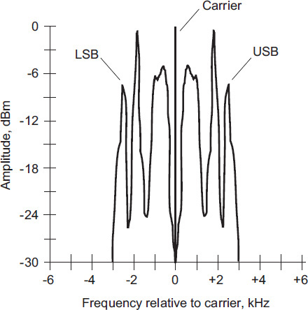
FIGURE 1-9 Spectral display of a typical amplitude-modulated (AM) voice communications signal.
Engineers define the bandwidth of any modulated signal as the difference between the maximum and minimum frequencies that the signal contains. In AM, the bandwidth always equals twice the highest audio modulating frequency, assuming that the transmitter is working properly. In the example of Fig. 1-9, all the audio input energy exists at or below 3 kHz, so the bandwidth of the modulated signal equals 6 kHz. That’s typical of AM voice communications. In AM broadcasting where music goes along with voices, the audio input energy gets spread over a wider bandwidth, nominally 10 kHz to 20 kHz. The increased bandwidth provides for better fidelity (sound quality) so that music doesn’t sound muffled in the receiver.
Single Sideband
As mentioned earlier, in an AM signal with 100% modulation, the carrier wave consumes 2/3 of the signal power, and the sidebands exist as mirror-image duplicates that, combined, take advantage of only 1/3 of the signal power.
Suppose that you could get rid of the carrier and one of the sidebands, but still convey all the information you want. In that case, you could get the same “signal bang” with far less transmitter power. Alternatively, you could get a stronger signal for the same amount of transmitter output power. You’d also reduce the signal bandwidth to just about half the bandwidth of an AM signal modulated with the same voice (actually, a little less with the carrier and one sideband completely gone). The resulting spectrum savings would allow you to fit more than twice as many signals into a specific range, or band, of frequencies, as you could do with AM. During the early twentieth century, communications engineers perfected a way to modify AM signals in precisely this way. They called the new communications mode single sideband (SSB), a term which endures to this day.
When you remove the carrier and one of the sidebands from an AM signal, the remaining energy has a spectral display resembling the graph of Fig. 1-10. In this case, the upper sideband (USB) energy along with the carrier wave has been eliminated, leaving only the lower sideband (LSB) energy. (You could, of course, just as well remove the LSB along with the carrier, leaving only the USB.) Radio hams make extensive use of both LSB and USB on their frequency bands, especially the ones below 30 MHz. They favor LSB at frequencies below 10 MHz, and USB at 10 MHz and above.
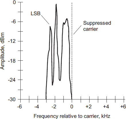
FIGURE 1-10 Spectral display of a hypothetical single-sideband (SSB) voice communications signal, in this case lower sideband (LSB).
Balanced Modulator
You can suppress the carrier in an AM signal using a balanced modulator, an amplitude modulator/amplifier using two transistors (or, in the olden days, vacuum tubes) with the inputs and outputs configured as shown in Fig. 1-11. This arrangement cancels out the carrier wave in the output signal, leaving only LSB and USB energy. The balanced modulator produces a double-sideband suppressed-carrier (DSBSC) signal, often called simply double sideband (DSB). You can suppress one of the sidebands in a subsequent circuit with the addition of a bandpass filter to obtain an SSB signal.
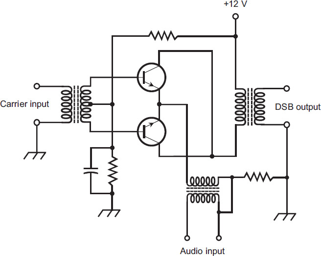
FIGURE 1-11 A balanced modulator using two transistors.
Basic SSB Transmitter
Figure 1-12 is a block diagram of a simple SSB transmitter. The RF amplifiers that follow any type of amplitude modulator, including a balanced modulator, must all operate in a linear manner to prevent distortion and unnecessary spreading of the signal bandwidth, a condition that some engineers and radio operators call splatter. The term linear refers to the fact that the amplifier output varies in direct proportion to the input, so that if you graph the output as a function of the input, you get a straight line.
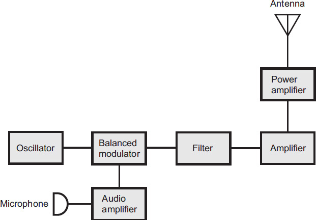
FIGURE 1-12 Block diagram of a basic SSB transmitter.
Frequency Modulation
In frequency modulation (FM), the instantaneous signal strength remains constant, and the instantaneous frequency varies. In the olden days of radio (and sometimes still today), engineers obtained FM by applying an audio signal to a varactor diode in a voltage-controlled oscillator (VCO). Figure 1-13 shows an example of this scheme, known as reactance modulation. The fluctuating voltage across the varactor causes its capacitance to change in accordance with the audio waveform. The fluctuating capacitance causes variations of the resonant frequency of the inductance-capacitance (LC) tuned circuit, causing small variations in the frequency generated by the oscillator. In the scenario of Fig. 1-13, the oscillator itself would be a so-called Colpitts circuit, which uses a split capacitance and a simple inductance.
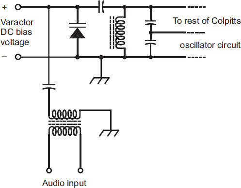
FIGURE 1-13 Generation of a frequency-modulated (FM) signal by means of reactance modulation.
Phase Modulation
You can indirectly obtain FM if you modulate the phase of an oscillator signal. That means you move the wave back and forth in time, without changing the frequency directly. However, when you vary the phase of a wave rapidly, you’ll get variations in the instantaneous frequency as an indirect consequence. As a matter of fact, any instantaneous phase change shows up as an instantaneous frequency change and vice versa. But there’s a glitch: When you employ so-called phase modulation (PM) with the intent of getting an FM signal, you must process the audio before you apply it to the modulator, adjusting the frequency response of the audio amplifiers by experiment. Otherwise the signal will sound distorted when you listen to it in a receiver designed for ordinary FM. Phase modulation is employed in many modern communications radios because it lends itself to the frequency synthesizers that have replaced tuned LC variable-frequency oscillators.
Deviation in FM and PM
In an FM or PM signal, the deviation is the maximum extent to which the modulated-carrier frequency rises above and falls below the unmodulated-carrier frequency. For most FM and PM voice transmitters, the deviation is standardized at ±5 kHz, a mode called narrowband FM (NBFM).
In NBFM, the signal bandwidth is roughly the same as that of an AM signal containing the same modulating information (your voice, for example). In hi-fi music broadcasting, and in some other applications, such as high-speed data transmission, the deviation exceeds ±5 kHz, a mode called wideband FM (WBFM).
The deviation obtainable with FM is greater for a given oscillator frequency than the deviation that you get with PM. However, you can increase the deviation of any FM or PM signal with a frequency multiplier. When the signal passes through a frequency multiplier, the deviation gets multiplied along with the carrier frequency itself.
Pulse-Amplitude Modulation
You can modulate a signal by varying some aspect of a sequence, or train, of signal bursts called pulses. In pulse-amplitude modulation (PAM), the amplitude (strength) of each individual pulse varies according to the modulating waveform. Figure 1-14A shows an amplitude-versus-time graph of a hypothetical PAM signal. The modulating waveform appears as a dashed curve, and the pulses appear as vertical gray bars. Normally, the pulse amplitude increases as the instantaneous modulating-signal level increases (positive PAM). But you can reverse the situation so that higher audio levels cause the pulse amplitude to go down (negative PAM). Then the signal pulses are at their strongest when there is no modulation. The transmitter has to work harder to produce negative PAM than it does to produce positive PAM. Either way, all the pulses all last for the same length of time. That is to say, they’re all equally wide.
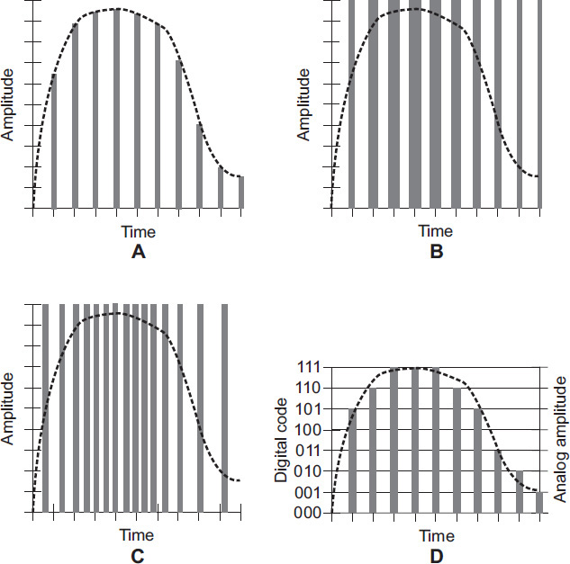
FIGURE 1-14 Time-domain graphs of various modes of pulse modulation. At A, pulse-amplitude modulation (PAM); at B, pulse-width modulation (PWM), also called pulse-duration modulation (PDM); at C, pulse-interval modulation (PIM); at D, pulse-code modulation (PCM).
Pulse-Width Modulation
You can modulate the output of an RF transmitter by varying the duration, or width, of the individual signal pulses to obtain pulse-duration modulation (PDM), also known as pulse-width modulation (PWM), as shown in Fig. 1-14B. Normally, the pulse width increases as the instantaneous modulating-signal level increases (positive PWM). But this situation can be reversed (negative PWM). The transmitter must work harder to accomplish negative PWM than to produce positive PWM because it has to transmit a signal for a larger proportion of the time on the average. Either way, the peak pulse amplitude remains constant; they’re all equally strong.
Pulse-Interval Modulation
Even if all the pulses have the same amplitude and the same duration, you can obtain pulse modulation by varying how often the pulses occur. In PAM and PWM, you always transmit the pulses at the same time interval, known as the sampling interval. But in pulse-interval modulation (PIM), pulses can occur more or less frequently than they do under conditions of no modulation. Figure 1-14C shows a hypothetical PIM signal. Every pulse has the same amplitude and the same duration, but the time interval between them changes. When the transmitted signal has no modulation, the pulses emerge evenly spaced with respect to time. An increase in the instantaneous data amplitude might cause pulses to be sent more often, as is the case in the illustration here (positive PIM). Alternatively, an increase in instantaneous data level might slow down the rate at which the pulses emerge (negative PIM). As with PWM, a transmitter must work harder to generate negative PIM than to produce positive PIM.
Pulse-Code Modulation
In digital communications, the modulating data attains only certain defined states, rather than continuously varying. Compared with old-fashioned analog communications (where the state is continuously variable), digital modes offer improved signal-to-noise (S/N) ratio, narrower signal bandwidth, better accuracy, and enhanced reliability. In pulse-code modulation (PCM), any of the above-described aspects—amplitude, width, or interval— of a pulse train can be varied. But rather than having infinitely many possible states, the number of states equals some power of 2, such as 22 (four states), 23 (eight states), 24 (16 states), 25 (32 states), 26 (64 states), and so on. As you increase the number of states, the fidelity improves, but the signal gets more “complicated.” Figure 1-14D shows an example of eight-level PCM. The amplitude levels are rendered as binary numbers from 000 (equivalent to the decimal number 0) to 111 (equivalent to the decimal number 7).
Receiver Fundamentals
A radio receiver converts radio waves into the original messages sent by a distant transmitter. Let’s define a few important criteria for receiver operation, and then we’ll look at a couple of common receiver designs.
Specifications
The specifications of a receiver quantify how well the hardware can carry out the tasks that its engineers designed and built it to do. Here are a few of the ones that you should think about before you buy a shortwave radio.
Sensitivity—The most common way to express receiver sensitivity is to state the number of signal microvolts (millionths of a volt) that must exist at the antenna terminals to produce a certain signal-to-noise ratio (S/N) or signal-plus-noise-to-noise ratio (S+N/N) in relative amplitude units called decibels (dB). The sensitivity depends on the gain of the front end (the amplifier that the signal enters from the antenna). The amount of noise that the front end generates also matters because subsequent stages amplify its noise output as well as its signal output.
Selectivity—The passband, or range of frequencies that the receiver can “hear,” is established by a wideband preselector in the early RF amplification stages, and is honed to precision by narrowband filters in later amplifier stages. A typical preselector makes the receiver most sensitive within a few percentage points of the desired signal frequency. The narrowband filter responds only to the frequency or channel of a specific signal that you want to hear, and rejects signals in nearby channels.
Dynamic range—The signals at a receiver input can vary over several orders of magnitude (powers of 10) in terms of absolute voltage. Engineers define dynamic range as the ability of a receiver to maintain a fairly constant output, and still keep its rated sensitivity, in the presence of signals ranging from extremely weak to extremely strong. A good receiver exhibits dynamic range in excess of 100 dB, which translates to a signal input power ratio of 10,000,000,000 to 1! A competent technician can conduct experiments to determine the dynamic range of any receiver.
Noise figure—As the amount of internal noise a receiver produces goes down, the S/N ratio improves, if all other factors remain constant. You can expect an excellent S/N ratio in the presence of weak signals only when your receiver has a low noise figure, which is a measure of internally generated circuit noise. The noise figure makes the most practical difference at VHF, UHF, and microwave frequencies. Gallium-arsenide field-effect transistors (GaAsFETs) are known for the low levels of electrical noise they generate at these frequencies. You can get away with other types of FETs at lower frequencies. Bipolar transistors, which carry higher currents than FETs, generate more circuit noise than FETs do.
Direct-Conversion Receiver
A direct-conversion receiver derives its output by mixing incoming signals with the output of a tunable (variable frequency) local oscillator (LO). The received signal goes into a circuit called a mixer along with the output of the LO, and the two signals beat against each other in the mixer. Figure 1-15 is a block diagram of a direct-conversion receiver.
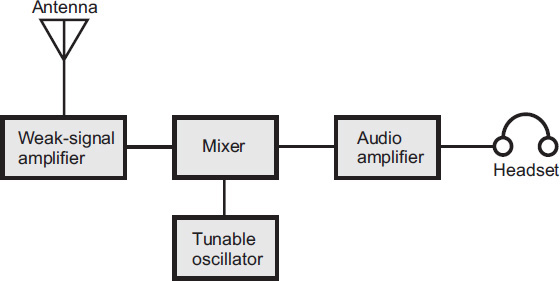
FIGURE 1-15 Block diagram of a direct-conversion receiver.
For reception of on/off keyed Morse code, the LO, which techies called a beat-frequency oscillator (BFO) before about 1980, is set a few hundred hertz above or below the signal frequency. You can also use this scheme to receive FSK signals. The audio output frequency equals the difference between the LO frequency and the incoming carrier frequency. For reception of AM or SSB signals, you must adjust the LO to precisely the same frequency as that of the signal carrier, a condition called zero beat because the beat frequency, or difference frequency, between the LO and the signal carrier is zero.
A direct-conversion receiver provides relatively poor selectivity, meaning that it can’t do a good job of separating signals when they lie close together in frequency. In a direct-conversion receiver, you can hear signals on either side of the LO frequency at the same time, and you can’t tell which one lies above the LO frequency and which one lies below it unless you adjust the tuning dial. Then one signal goes up in pitch and the other goes down, a weird and rather maddening effect to some folks. A selective filter can theoretically eliminate this problem. Such a filter must be designed for a fixed frequency if you expect it to work well. However, in a direct-conversion receiver, the RF amplifier must operate over a wide range of frequencies, making effective filter design an engineering challenge.
Superheterodyne Receiver
A superheterodyne receiver, also called a superhet, uses one or more LOs along with signal mixers to obtain a constant-frequency signal. You can more easily filter a fixed-frequency signal than you can filter a signal that changes in frequency (as it does in a direct-conversion receiver). A mixer produces output signals at the sum and difference frequencies of the input signals.
In a superhet, the incoming signal goes from the antenna through a tunable, sensitive front end, which comprises a precision weak-signal amplifier. The output of the front end mixes (heterodynes) with the signal from a tunable, unmodulated LO. You can choose the sum signal or the difference signal for subsequent amplification. Engineers call this signal the first intermediate frequency (IF), which can be filtered to obtain enhanced selectivity.
If the first IF signal passes straight into the detector (signal demodulator), you have a single-conversion receiver. Some receivers use a second mixer and second LO, converting the first IF to a lower-frequency second IF. Then you have a double-conversion receiver. The IF bandpass filter can be constructed for use on a fixed frequency, allowing superior selectivity and facilitating adjustable bandwidth. The sensitivity is enhanced because fixed-frequency IF amplifiers are easy to keep in tune. In a double-conversion receiver, the low second IF makes it possible to obtain better selectivity than can normally be obtained with a single-conversion design.
Stages of a Single-Conversion Superhet
Figure 1-16 shows a block diagram of a single-conversion superheterodyne receiver. Individual receiver designs vary, but you can consider this example representative. The stages break down as follows:
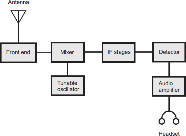
FIGURE 1-16 Block diagram of a single-conversion superheterodyne receiver.
• The front end serves as the first RF amplifier, and may include a bandpass filter between the amplifier and the antenna. The dynamic range and sensitivity of a receiver are determined largely by the performance of the front end.
• The mixer stage, in conjunction with the tunable LO, converts the variable signal frequency to a constant IF. The output occurs at either the sum or the difference of the signal frequency and the LO frequency.
• The IF stages produce most of the gain (amplification) in a superhet receiver. You also get most of the selectivity here, filtering out unwanted signals and noise while allowing the desired signal to pass.
• The detector extracts the information from the signal. Common circuits include the envelope detector for AM, the product detector for SSB, FSK, and CW, and the ratio detector for FM and PM. You’ll find explanations of these system elements later in this chapter.
• The audio amplifier boosts the demodulated signal to a level suitable for a speaker or headset. Alternatively, you can feed the signal to a printer, facsimile machine, computer, or other device.
Predetector Stages
When you design and build a superheterodyne receiver, you must ensure that the stages preceding the first mixer provide reasonable gain but generate minimal internal noise. They must also be able to bring in strong signals without desensitization (losing gain), a phenomenon also known as overloading.
Preamplifier
If a receiver doesn’t have enough sensitivity to satisfy you, you can use a preamplifier between the antenna and the radio. Figure 1-17 shows a simple preamplifier circuit that can use either a junction field-effect transistor (JFET) or a GaAsFET. Input tuning reduces noise and provides some selectivity. This circuit produces 5 dB to 10 dB of useful signal gain, depending on the frequency and the choice of FET.
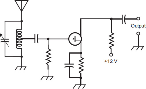
FIGURE 1-17 A tunable preamplifier. Normally, this type of amplifier uses a JFET or GaAsFET, and goes between the antenna and the front end of the radio.
You must make sure that your preamplifier remains linear in the presence of strong input signals. Nonlinearity can cause unwanted mixing among multiple incoming signals. These so-called mixing products produce intermodulation distortion (IMD) or intermod that can spawn multiple images inside the receiver. Intermod can also degrade the S/N ratio by generating hash, a form of wideband RF noise.

Front End
At low and medium frequencies, considerable atmospheric noise exists, and the design of a front-end circuit is simple because you don’t have to worry very much about internally generated noise. Conditions are bad enough in the antenna feed line as it comes into your receiver; a little more noise coming from inside the radio itself won’t likely matter.
Atmospheric noise diminishes as you get above 30 MHz or so. Then the main sensitivity-limiting factor becomes noise generated within the receiver. For this reason, front-end design grows in importance as the frequency rises through the VHF, UHF, and microwave parts of the radio spectrum.
The front end, like a preamplifier, must remain as linear as possible. In other words, it mustn’t introduce distortion. The greater the degree of nonlinearity, the more susceptible the circuit becomes to the generation of mixing products and intermod. The front end should also have the greatest possible dynamic range.
Preselector
A preselector, if the radio has one, provides a bandpass response that improves the S/N ratio, and reduces the likelihood of overloading by a strong signal that’s far removed from the operating frequency. The preselector also provides some extra image rejection in a superheterodyne circuit. You can tune a preselector by means of tracking with the receiver’s main tuning control, but this technique requires careful design and alignment. Some older receivers incorporate preselectors that must be adjusted independently of the receiver tuning.
IF Chains
A high IF (at least several megahertz) works better than a low IF for image rejection. However, a low IF allows for superior selectivity. Double-conversion receivers use two mixers and two IF chains. The comparatively high first IF and low second IF give you the “best of both worlds.” The designers of these receivers cascade multiple IF amplifiers (connect them one after the other). There are two sets, called chains, of IF amplifiers. The first IF chain follows the first mixer and precedes the second mixer, and the second IF chain follows the second mixer and precedes the detector.
Engineers sometimes express IF-chain selectivity by comparing the bandwidths for two power-attenuation (amplitude-reduction) values, usually −3 dB and −30 dB, also called 3 dB down and 30 dB down. This specification offers a good description of the bandpass response. You call the ratio of the bandwidth at −30 dB to the bandwidth at −3 dB the shape factor. In general, small shape factors are more desirable than large ones, but small shape factors are more difficult to attain in practice.
Detectors
Detection, also called demodulation, allows a radio receiver to recover the modulating information, such as audio, images, or printed data, from an incoming signal.
Detection of AM
A radio receiver can extract the information from an AM signal by “chopping off” either the positive or the negative part of the carrier wave (in other words, rectifying it), and then filtering the output waveform just enough to smooth out the RF pulsations. Figure 1-18A shown a simplified time-domain view of how this process works. The rapid pulsations (solid curves) occur at the RF carrier frequency; the slower fluctuation (dashed curve) portrays the modulating data. The carrier pulsations get smoothed out as the output passes through a capacitor large enough to hold the charge for one carrier current cycle, but not so large that it dampens or obliterates the fluctuations in the modulating signal. Engineers call this technique envelope detection.
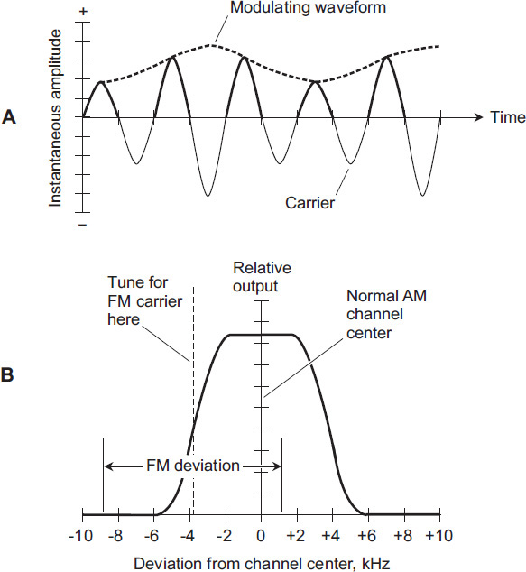
FIGURE 1-18A-B At A, envelope detection of AM, shown in the time domain (a graph of amplitude versus time). At B, slope detection of FM, shown in the frequency domain (a graph of amplitude versus frequency).
Detection of CW and FSK
If you want a receiver to detect CW signals, you must inject a constant-frequency, unmodulated carrier a few hundred hertz above or below the signal frequency. The local carrier is produced by a tunable LO inside the receiver. The LO signal and the incoming CW signal beat against each other in a mixer to produce audio output at the sum or difference frequency. You can tune the LO to obtain an audio note at a comfortable listening pitch, usually 500 to 1000 Hz. This process is called heterodyne detection.
You can detect FSK signals using the same method as CW detection. The carrier beats against the LO in the mixer, producing an audio tone that alternates between two different pitches. With FSK, the LO frequency is set a few hundred hertz above or below both the mark frequency and the space frequency. The frequency offset, or difference between the LO and signal frequencies, determines the audio output frequencies. You adjust the frequency offset to get specific standard AF notes (such as 2125 Hz and 2295 Hz in the case of 170-Hz shift).
Slope Detection of FM and PM
You can use an AM receiver to detect FM or PM by setting the receiver frequency near, but not exactly at, the unmodulated-carrier frequency. An AM receiver has a filter with a passband of a few kilohertz and a selectivity curve, such as the one shown in Fig. 1-18B. If you tune the receiver so that the FM unmodulated-carrier frequency lies near either edge, or skirt, of the filter response, frequency variations in the incoming signal cause its carrier to swing in and out of the receiver passband. As a result, the instantaneous receiver output amplitude varies along with the modulating data on the FM or PM signal. In this system, known as slope detection, a nonlinear relationship exists between the instantaneous deviation and the instantaneous output amplitude because the skirt of the passband does not produce a straight line in a graph of amplitude versus frequency.
Discriminator for FM or PM
A discriminator produces an output voltage that depends on the instantaneous signal frequency. When the signal frequency lies at the center of the receiver passband, the output voltage equals zero. When the instantaneous signal frequency falls below the passband center, the output voltage becomes positive. When the instantaneous signal frequency rises above center, the output voltage becomes negative.
In a discriminator circuit, you get a linear relationship between the instantaneous deviation of the FM (which can result indirectly from PM) and the instantaneous output amplitude. Therefore, the detector output represents a faithful reproduction of the incoming signal data. A discriminator will respond to amplitude variations, but you can use an amplitude limiting circuit to overcome this effect if it poses a problem.
Ratio Detector for FM or PM
A ratio detector comprises a discriminator with a built-in limiter. The original design was developed by RCA (Radio Corporation of America), and works well in hi-fi receivers and in the audio portions of old-fashioned analog TV receivers. Figure 1-18C illustrates a ratio detector circuit. The potentiometer marked “balance” must be adjusted experimentally to get optimum received-signal audio quality.
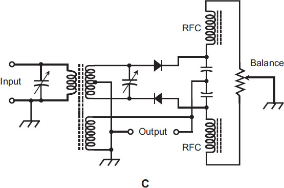
FIGURE 1-18C At C, a ratio detector circuit for demodulating FM signals.
Detection of SSB
For reception of SSB signals, most communications engineers favor a product detector, although a direct-conversion receiver can do the job. A product detector also facilitates reception of CW and FSK. The incoming signal combines in a mixer with the output of an unmodulated LO, reproducing the original modulating signal data. Product detection occurs at a single frequency, rather than at a variable frequency that is characteristic of direct-conversion reception.
Figures 1-18D and E show product-detector circuits, which can also serve as mixers in superheterodyne receivers. In the circuit at D, diodes are used. They’re passive components, so you don’t get any amplification. The circuit at E employs a single-transistor amplifier, providing some gain if the incoming signal has been sufficiently amplified by the front end before it arrives at the detector input.
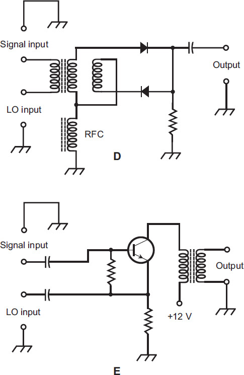
FIGURE 1-18D-E At D, a product detector using diodes. At E, a product detector using an NPN bipolar transistor biased as a class-B amplifier.
The effectiveness of the circuits shown in Figs. 1-18D or E lies in the nonlinearity of the semiconductor devices. The nonlinearity facilitates (and, in fact, encourages) the heterodyning that’s necessary to obtain sum and difference frequency signals that result in data output. So, as you can see, nonlinearity isn’t always bad. Sometimes you want a circuit to be nonlinear!
Audio Filtering
In a communications system, a human voice signal requires a band of frequencies ranging from about 300 Hz to 3000 Hz for a listener to easily understand the content. An audio bandpass filter, with a passband of 300 Hz to 3000 Hz, can improve the intelligibility in some voice receivers. An ideal voice audio bandpass filter has little or no attenuation within the passband range but high attenuation outside the passband range, along with a near-rectangular response curve.
A CW or FSK signal requires only a few hundred hertz of bandwidth. Audio CW filters can narrow the response bandwidth to 100 Hz or less, but passbands narrower than about 100 Hz produce ringing, degrading the quality of reception at high data speeds. With FSK, the bandwidth of the filter must be at least as large as the difference (shift) between mark and space, but it need not (and shouldn’t) greatly exceed the frequency shift.
An audio notch filter is a band-rejection filter with a sharp, narrow response. Band-rejection filters pass signals only below a certain lower cutoff frequency or above a certain upper cutoff frequency. Between those limits, in the so-called bandstop range, signals are blocked. A notch filter can mute an interfering unmodulated carrier or CW signal that produces a constant-frequency tone in the receiver output. Audio notch filters are tunable from at least 300 Hz to 3000 Hz. A good notch filter has an extremely narrow bandstop range, so you can get rid of an unwanted carrier signal with minimal adverse effect on the rest of the audio range.
Squelching
A squelch silences a receiver when no incoming signals exist, allowing reception of signals when they appear. Most FM communications receivers use squelching systems. The squelch is normally closed, cutting off all audio output (especially receiver hiss, which annoys some communications operators) when no signal is present. The squelch opens, allowing everything to be heard, if the signal amplitude exceeds a squelch threshold that the operator can adjust.
In some radios, the squelch does not open unless an incoming signal has certain predetermined characteristics. This feature is called selective squelching. The most common way to achieve selective squelching is the use of a subaudible (below 300 Hz) tone generator or audio tone-burst generator in the transmitter. The squelch opens only in the presence of signals modulated by an audio tone, or sequence of tones, having the proper characteristics. Some radio operators use selective squelching to prevent unwanted transmissions from coming in.
Exotic Communications Methods
Communications engineers have a long history of innovation, developing alternative (and some downright weird) wireless modes. In recent years, new modes have emerged; you can expect more to come, each of which offers specific advantages under strange or difficult conditions. Four common examples follow.
Dual-Diversity Reception
A dual-diversity receiver can reduce fading in radio reception at frequencies between approximately 3 MHz and 30 MHz when signals propagate through the ionosphere and return to earth’s surface. The system comprises two identical receivers tuned to the same signal and having separate antennas spaced several wavelengths apart. The outputs of the receiver detectors go into a single audio amplifier, as shown in Fig. 1-19.
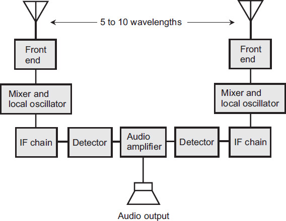
FIGURE 1-19 Block diagram of a diversity radio reception system.
Dual-diversity receiver tuning is a sophisticated technology (you might call it an art), and good equipment for this purpose costs a lot of money. Some advanced diversity-reception installations employ three or more antennas and receivers, providing superior immunity to fading, but further compounding the tuning difficulty and driving up the expense.
Synchronized Communications
Digital signals require less bandwidth than analog signals to convey a given amount of information per unit of time. The term synchronized communications refers to any of several specialized digital modes in which the transmitter and receiver operate from a common frequency-and-time standard to optimize the amount of data that can be sent in a communications channel or band.
In synchronized digital communications, also called coherent communiations, the receiver and transmitter operate in lockstep. The receiver evaluates each transmitted data bit for a block of time lasting for the specified duration of a single bit. This process makes it possible to use a receiving filter having extremely narrow bandwidth. The synchronization requires the use of an external frequency-and-time standard, such as that provided by the National Institute of Standards and Technology (NIST) radio station WWV in the United States. Frequency dividers generate the necessary synchronizing signals from the frequency-standard signal. A tone or pulse appears in the receiver output for a particular bit if, but only if, the average signal voltage exceeds a certain value over the duration of that bit. False signals caused by filter ringing, atmospheric noise, or ignition noise are generally ignored, because they rarely produce sufficient average bit voltage.
Multiplexing
Signals in a communications channel or band can be intertwined, or multiplexed, in various ways. The most common methods are frequency-division multiplexing (FDM) and time-division multiplexing (TDM). In FDM, the channel is broken down into subchannels. The carrier frequencies of the signals are spaced so that they don’t overlap. Each signal remains independent of all the others. A TDM system breaks signals down into segments of specific time duration, and then the segments are transferred in a rotating sequence. The receiver stays synchronized with the transmitter by means of an external time standard, such as the data from WWV.
Spread Spectrum
In spread-spectrum communications, the transmitter varies the main carrier frequency in a controlled manner, independently of the signal modulation. The receiver is programmed to follow the transmitter frequency from instant to instant. The whole signal therefore roams up and down in frequency within a defined range.
In spread-spectrum mode, the probability of catastrophic interference, in which one strong unwanted signal can obliterate the desired signal, is near zero. Unauthorized people find it impossible to eavesdrop on a spread-spectrum communications link unless they gain access to the sequencing code, also known as the frequency-spreading function. Such a function can be complicated indeed. As long as neither the transmitting operator nor the receiving operator divulge the sequencing code to anyone else, then (ideally) no unauthorized listener can intercept it.
During a spread-spectrum contact between a given transmitter and receiver, the operating frequency can fluctuate over a range of several kilohertz, megahertz, or tens of megahertz. As a band becomes occupied with an increasing number of spread-spectrum signals, the overall noise level in the band appears to increase. Therefore, a practical limit exists to the number of spread-spectrum contacts that a band can handle. This limit is roughly the same as it would be if all the signals were constant in frequency, and had their own discrete channels. The main difference between fixed-frequency communications and spread-spectrum communications, when the band gets crowded, lies in the nature of the mutual interference.
A common method of generating spread-spectrum signals involves so-called frequency hopping. The transmitter has a list of channels that it follows in a certain order. The transmitter jumps from one frequency to another in the list. The receiver must be programmed with this same list, in the same order, and must be synchronized with the transmitter. The dwell time equals the length of time that the signal remains on any given frequency; it’s the same as the time interval at which frequency changes occur. In a well-designed frequency-hopping system, the dwell time is short enough so that an unauthorized listener using a receiver set to a constant frequency won’t notice it. In addition, the signal should not dwell on any frequency long enough to cause interference with a fixed signal that happens to lie on that frequency. The transmitter sequence contains numerous dwell frequencies, so the signal energy gets diluted to the extent that, if someone tunes to any particular frequency in the sequence, they won’t notice the signal.
Another way to obtain spread-spectrum emission, called frequency sweeping, requires frequency-modulating the main transmitted carrier with a waveform that guides it smoothly up and down in frequency over the assigned band. The “sweeping FM” remains entirely independent of the actual data that the signal conveys. A receiver can intercept the signal if, but only if, its instantaneous frequency varies according to the same waveform, over the same band, at the same rate, and in the same phase as that of the transmitter. The transmitter and receiver in effect roam all over the band, following each other from moment to moment according to a “secret map” that only they know.