Generative Adversarial Networks (GANs) have gained a lot of popularity since their first introduction in a 2014 NIPS paper by Ian Goodfellow and their co-authors (https://arxiv.org/pdf/1406.2661.pdf). Now we see applications of GANs in various domains. Researchers from Insilico Medicine proposed an approach to artificial drug discovery using GANs. They also found applications in image processing and video processing problems, such as image style transfers and deep convolutional generative adversarial networks (DCGAN). 

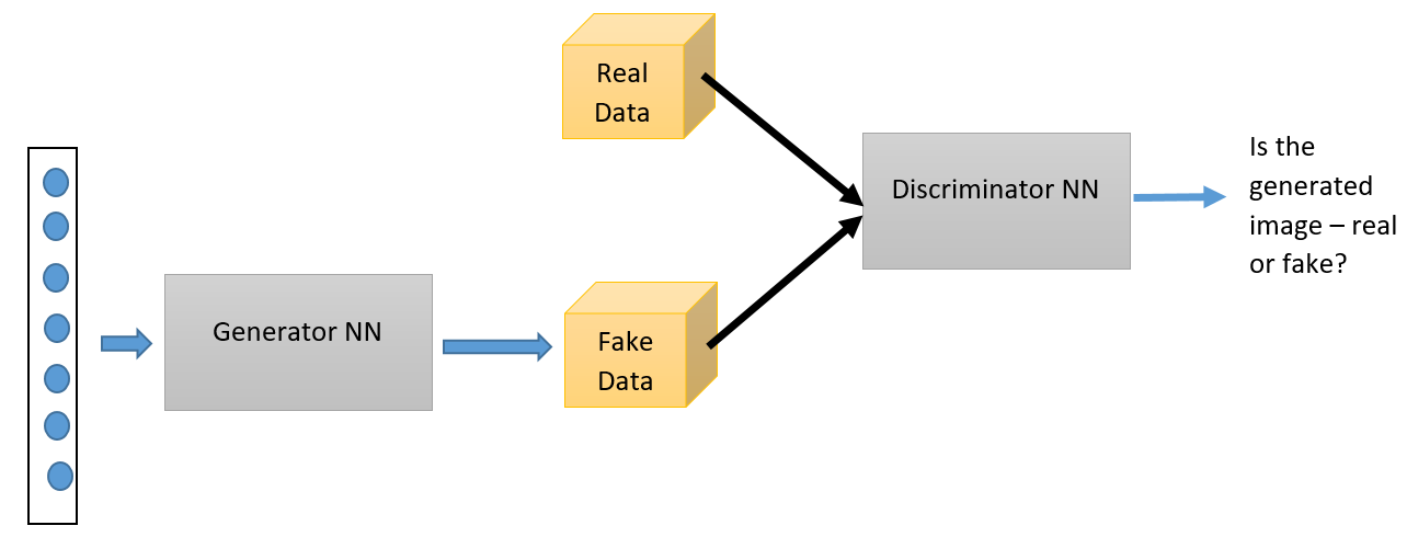
As the name suggests, this is another type of generative model that uses neural networks. GANs have two main components—a generator neural network and a discriminator neural network. The generator network takes a random noise input and tries to generate a sample of data. The discriminator network compares the generated data with the real data and solves the binary classification problem of whether generated data is fake or not, using sigmoid output activation. Both the generator and the discriminator are constantly competing and trying to fool each other—that's the reason that GANs are also known as adversarial networks. This competition drives both the networks to improve their weights until the discriminator starts outputting a probability of 0.5; that is, until the generator starts generating real images. Both the networks are trained simultaneously by backpropagation. Here is a high-level structural diagram of a GAN:

The loss function for training these networks can be defined as follows. Let pdata be the probability distribution of the data and pg be the generator distribution. D(x) represents the probability that x came from pdata and not from pg. D is trained to maximize the probability of assigning the correct label to both training examples and samples from G. Simultaneously, G is trained to minimize log(1 − D(G(z))). So, D and G play a two-player minimax game with value function V(D, G):

It can be proved that this minimax game has a global optimum for p_g = p_data. 

The following is the algorithm for training a GAN with backpropagation to obtain the desired result:

for N epochs do:

    #update discriminator net first

    for k steps do:

          Sample minibatch of m noise samples {z(1), , . . . , z  
          (m)} from noise prior pg(z).

           Sample minibatch of m examples {x(1), . . . , x(m)} from  
           data generating distribution pdata(x).

           Update the discriminator by: 

               
    end for

         Sample minibatch of m noise samples {z(1) , . . . , z (m)}  
         from noise prior pg(z).
         Update the generator by descending its stochastic gradient:
               

end for