Since this chapter and book is focused upon transfer learning, let's quickly get on with the actual task of leveraging and transferring learned information. We have discussed different state-of-the-art CNN architectures in the previous section. Let's now leverage the VGG-16 model, trained on ImageNet, to classify images from the CIFAR-10 dataset. The code for this section is available in the IPython Notebook CIFAR10_VGG16_Transfer_Learning_Classifier.ipynb.
ImageNet is a huge visual dataset with over 20,000 different categories. CIFAR-10, on the other hand, is restricted to only 10 non-overlapping categories. A powerful network like VGG-16 requires immense computational power and time to train to perform better than humans. This brings transfer learning into the picture. Since most of us do not have access to unlimited compute, we can leverage these networks under two distinct settings:
- Use pretrained state-of-the-art networks as feature extractors. This is done by removing the top classification layer and using the output from the penultimate layer.
- Fine-tuning the state-of-the-art network on the new dataset.
We will utilize VGG-16 as a feature extractor and build a custom classifier on top of it. The following snippet loads and prepares the CIFAR-10 dataset for use:
# extract data
(X_train, y_train), (X_test, y_test) = cifar10.load_data()

#split train into train and validation sets
X_train, X_val, y_train, y_val = train_test_split(X_train,
                                                  y_train,
                                                  test_size=0.15,
                                                  stratify=np.array
                                                            (y_train),
                                                  random_state=42)

# perform one hot encoding
Y_train = np_utils.to_categorical(y_train, NUM_CLASSES)
Y_val = np_utils.to_categorical(y_val, NUM_CLASSES)
Y_test = np_utils.to_categorical(y_test, NUM_CLASSES)

# Scale up images to 48x48
X_train = np.array([sp.misc.imresize(x,
                                     (48, 48)) for x in X_train])
X_val = np.array([sp.misc.imresize(x,
                                   (48, 48)) for x in X_val])
X_test = np.array([sp.misc.imresize(x,
                                    (48, 48)) for x in X_test])
The preceding code snippet not only splits the training dataset into train and validation sets, but also transforms the target variable into one-hot encoded form. We also resize the images to 48 x 48 from 32 x 32, to comply with VGG-16 input requirements. Once the train, validation, and test datasets are ready, we can work toward preparing our classifier.
The following code snippet shows how easily we can attach a new layer(s) on top of an existing model. As our objective is to train the classification layer only, we freeze the rest of the layers by setting the parameter trainable to False. This allows us to leverage the existing architectures even on less powerful infrastructures, and transfer the learned weights from one domain to another:
base_model = vgg.VGG16(weights='imagenet',
include_top=False,
input_shape=(48, 48, 3))

# Extract the last layer from third block of vgg16 model
last = base_model.get_layer('block3_pool').output

# Add classification layers on top of it
x = GlobalAveragePooling2D()(last)
x= BatchNormalization()(x)
x = Dense(64, activation='relu')(x)
x = Dense(64, activation='relu')(x)
x = Dropout(0.6)(x)
pred = Dense(NUM_CLASSES, activation='softmax')(x)
model = Model(base_model.input, pred)

for layer in base_model.layers:
layer.trainable = False
We have the basic ingredients in place. One final block remaining in this overall pipeline is data augmentation. The overall dataset contains just 60,000 images; data augmentation comes in handy to add certain variations to the sample set at hand. These variations enable the network to learn more generalized features than otherwise. The following code snippet utilizes the ImageDataGenerator() utility to prepare train and validation augmentation objects:
# prepare data augmentation configuration
train_datagen = ImageDataGenerator(rescale=1. / 255,
                                   horizontal_flip=False)

train_datagen.fit(X_train)
train_generator = train_datagen.flow(X_train,
                                     Y_train,
                                     batch_size=BATCH_SIZE)

val_datagen = ImageDataGenerator(rescale=1. / 255,
                                 horizontal_flip=False)

val_datagen.fit(X_val)
val_generator = val_datagen.flow(X_val,
                                 Y_val,
                                 batch_size=BATCH_SIZE)
Let's now train the model for a few epochs and measure its performance. The following code snippet calls the fit_generator() function to train the newly added layer to the model:
train_steps_per_epoch = X_train.shape[0] // BATCH_SIZE
val_steps_per_epoch = X_val.shape[0] // BATCH_SIZE

history = model.fit_generator(train_generator,
                              steps_per_epoch=train_steps_per_epoch,
                              validation_data=val_generator,
                              validation_steps=val_steps_per_epoch,
                              epochs=EPOCHS,
                              verbose=1)
The history object returned by fit_generator() contains details about each epoch. We utilize these to plot the overall model performance in terms of accuracy and loss. The results are shown as follows:

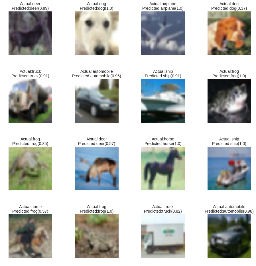
As we can see, transfer learning has helped us achieve an amazing boost in the overall performance, compared to the model developed from scratch. This improvement utilized trained weights of VGG-16 to transfer the learned features to this domain. Readers can utilize the same utility plot_predictions() to visualize classification results on a random sample, as shown in the following screenshot:

This was a quick and simple application of transfer learning, where we utilized an amazingly complex deep CNN like VGG-16 to prepare a CIFAR-10 classifier. Readers are encouraged to try out not just different configurations of the custom classifier, but rather to even try out different pretrained networks to understand the complexities involved.
