Chapter 10

HOW ROUND IS YOUR CIRCLE?

Round and round the rugged rock the ragged rascal ran.

Nursery rhyme

 

 

Imagine you wish to make a circular or spherical object but cannot simply use compasses to mark one out. Alternatively, you might have already made something round and wish to check the accuracy of your construction. We all know what a circle is, so here we discuss the problem of determining if what is supposed to be circular is really circular, and within what limits. This matters a lot in engineering applications of all sorts but particularly with rotating shafts and their bearings.

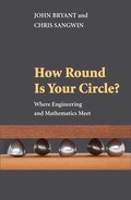
So let us begin with an experiment for which you need a United Kingdom 50p (or 20p) coin, a 2p coin and, if possible, a new round beer mat or coaster. You will also need the means to measure their widths—Vernier callipers are ideal, but you can just about manage with a clearly graduated rule. Merely glancing at these objects is enough to see that the 2p coin and the beer mat are round and that the 50p piece is certainly not. The next step is to measure their widths, or diameters, in as many orientations as possible. Both coins had constant width, whereas our beer mat had a width varying between 106.1 and 106.5 mm. What can we deduce from these observations and measurements?

The 50p piece as shown in figure 10.1 is obviously not circular, and yet it does have constant width. The beer mat, although appearing to be circular, cannot be because the width varies, and nothing can be said of the 2p coin at this stage except that it might be circular but we do not know for sure. We dismissed the 50p as not round, but what if it had had 77 or 777 sides, still with constant width? It might then have seemed round, but all we can say is that constant width is a necessary condition for roundness but by itself it is not sufficient. The 2p might be round, but without further tests we cannot be sure. Incidentally, the fact that a 50p piece has constant width is a useful geometric property which helps reduce the number of times such coins get stuck in slot machines.

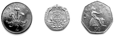
Figure 10.1. United Kingdom coins: 2p, 20p and 50p.

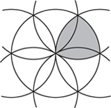
Figure 10.2. Constructing Reuleaux’s rotor.

If you do not have access to these coins, you can make three planar shapes yourself and conduct another experiment. The first is a circle, the second is a square and the third is a slightly unusual shape which can be made easily using the technique that follows—and it is really only a minor variation of figure 5.3. Start with a pair of compasses open and draw a circle. Mark an arbitrary point on the circle and using this as a centre draw another circle. Then draw further circles, all with the same radius, where previously drawn circles intersect (see figure 10.2).

If you focus your attention on the circular arcs, you will notice the shape we have highlighted in grey. There are, of course, six overlapping copies of this shape in the circle. Alternatively, you can construct this shape from an equilateral triangle by drawing circular arcs centred at each vertex passing through the other two. It is known as Reuleaux’s rotor, after Franz Reuleaux (1829–1905), and is shown as both a schematic and a model in figure 10.3. Historically, the first author to mention such shapes of which we are aware is Euler (1778).

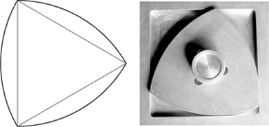
Figure 10.3. Reuleaux’s rotor.

You probably do not actually need to perform the experiment to determine that the width of the circle is constant. Geometrical intuition, together with the Pythagorean theorem, should help you to establish easily that the width of the square varies between 1 and times the length of the side. What about Reuleaux’s rotor?

It is easy to see that Reuleaux’s rotor also has constant width. A tangent to one of the circular arcs will be at a constant distance from a parallel line through the centre of this arc.

This experiment sets the scene for this chapter, where first we discuss the infinite family of closed convex curves of constant width, some of their applications, and how to make examples. We then move on to the more difficult question of how roundness can be measured and why it matters.

A circular cross-section is the most frequently used basic shape in engineering. We define a shape to be round if it has a circular cross-section. This is only the case if all points on the boundary are equidistant from the centre, or axis. When measuring the width of the shape we did not make use of an axis, and indeed non-circular shapes of constant width do not possess one. While they can be used as rollers they cannot become true wheels.

Engineers are most concerned with measuring departure from roundness. This is a particularly important engineering problem, since many devices depend on rotation. The most important device is the bearing that allows a shaft to rotate smoothly. In a plain bearing a shaft rotates and it is vital to obtain the correct clearance to allow smooth running in the presence of lubrication. More complex types of bearing, such as ball bearings or roller bearings, also depend critically on the roundness of their components.

While the straightness or flatness of an object can be checked against a reference surface, as detailed in section 1.5, this is much more difficult for roundness. In manufacturing it is probably true to say that departures from true roundness present the greatest difficulties of all the form errors that have to be evaluated. In this chapter we shall examine shapes of constant width in two and three dimensions, provide some practical applications of these shapes beyond coin design, and then explain how departure from roundness can be measured.

10.1 Families of Shapes of Constant Width

After the circle the simplest curve of constant width is Reuleaux’s rotor, sometimes called Reuleaux’s ‘triangle’. We shall begin with a variety of families of two-dimensional shapes of constant width. In each of the families there is a spectrum of variation with Reuleaux’s rotor at one extreme and the circle at the other. Either the number of sides in a polygon increases or there is continuous change of an arc’s radius or construction angle to create this spectrum. Furthermore, all these methods rely on the use of circular arcs to make up the shapes.

The first method is a simple generalization of that used to create a Reuleaux rotor. Start with any regular polygon with an odd number of sides. Draw a circular arc centred at one vertex that passes through the two opposite vertices. The Reuleaux rotor is one example, starting with the regular equilateral triangle. As the number of sides increases so the shapes come closer to true circles, although all these shapes have sharp corners. It is relatively easy to extend the lines from the regular polygons and draw two circular arcs to create a more general form of the Reuleaux rotor. Of course, this can also be done with all the regular polygons. The resulting shapes are now smooth, and all have constant width. This is shown in the left column of figure 10.4

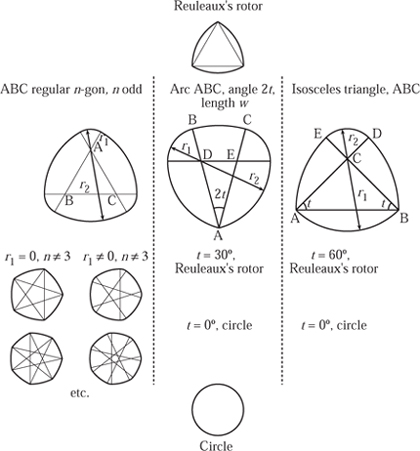
Figure 10.4. Families of shapes of constant width.

A different family of shapes can be developed, as shown in the middle column of figure 10.4. This family includes a sector of a circle of radius w with angle 2t. The positions of D and E are determined by simple geometry such that r₁ + r₂ = w with If t = 0° then the resulting shape is a circle of diameter w, and if t = 30° then we have a Reuleaux rotor.

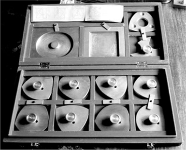
Figure 10.5. A collection of shapes of constant width by G. J. H. Cordle as a final year undergraduate project in 1995.

The final family is based on an isosceles triangle and is shown in the right column of figure 10.4. We take A and B to be a distance w apart and draw the isosceles triangle ABC with angles t at A and B. Hence, we have that

This shape is unusual in that it is composed of only four circular arcs. The angle t = 45° is a special case and forms the basis of a drill that creates a square hole, which we shall describe in section 10.4.

10.2 Other Shapes of Constant Width

Just in case you harbour any lingering doubt that shapes of constant width, such as the Reuleaux rotor, are a ‘special trick’, we shall provide yet more examples. These need not have any symmetries. Let us start with any three lines that form a triangle ABC as shown in figure 10.6. Choose another point D on the line AB, external to the triangle, and draw the arc centred at A through D between the lines AB and AC. Then proceed round the circle connecting each arc with the preceding one, centring the arc at the intersection of the lines that it connects. There is a feasibility constraint: for example, if D is too close to A then the arc centred at B will fall between A and C. This constraint can always be satisfied by making the distance AD sufficiently large, and if so the resulting shape has constant width. This procedure may be done with an arbitrary number of mutually intersecting lines, and it results in shapes with an arbitrary number of different circular arcs.

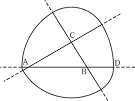
Figure 10.6. Building a shape of constant width from an arbitrary triangle ABC.

It is worth making some general comments about all the shapes so far constructed. It can readily be verified by adding the lengths of circular arcs in all these examples that the length of the perimeter of the shape is wπ. This, of course, is identical to the circumference of the circle with diameter (i.e. width) w. In fact, a theorem of Barbier, proved rigorously in Lyusternik (1964), demonstrates that all curves of constant width w have an identical perimeter length of wπ.

The Reuleaux rotor is in many senses the most extreme shape of constant width. It has the smallest area for a given width w, which equals w²(π - ). It also has the sharpest corners, where tangents meet at an angle of 120°. The circle has the largest area for a given width and all other constant-width shapes must fall somewhere in between.

All the curves constructed so far have been built piecewise from circular arcs, but this is not a necessary condition. Now we turn our attention to even more general methods for creating shapes of constant width that do not rely on circular arcs. Start with a square of width w and draw a convex curve from top to bottom that touches the left-hand side and that is tangent to the top and bottom of the square. At no point should the curvature be less than the curvature of a circle with radius w. We can, in a sense, ‘complete’ the curve to create a shape of constant width by taking a normal to the curve of length w. This can be done by hand with a ruler very quickly, and reasonably accurately.

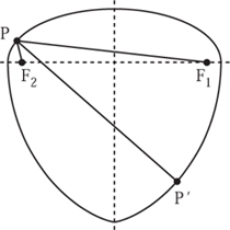
Figure 10.7. A curve of constant width, based on half an ellipse.

As an example of this method we shall create a curve based on one-half of an ellipse:

To start we take only the half with y > 0, as shown in figure 10.7. At a point P construct the inward-facing normal PP′ of length w. The bottom half is given by the locus of P′ as P moves around the top. Figure 10.7 shows the case when b = a = w, its minimum possible value. We shall deal more fully with ellipses and their various properties, and explain how to construct the normal to an ellipse, in chapter 13.

There is a limit to the eccentricity of the ellipse used in this construction. The radius of curvature at (0,b) is a²/b, and the maximum value this can take is 2a, the length of the major axis, otherwise a convex curve of constant width cannot be constructed. As b increases towards a the whole curve approaches a circle. The limit of a Reuleaux rotor cannot be reached with this particular construction. In section 10.9 we shall provide another method that has the advantage of providing mathematical expressions for the shapes produced and with which we can perform some quantitative calculations of the departures from roundness.

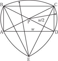
Figure 10.8. Generating a three-dimensional shape with a spherical cross-section.

10.3 Three-Dimensional Shapes of Constant Width

A solid may also have constant width. The simplest of these is formed by rotating the Reuleaux rotor about an axis of symmetry. Indeed, any of the shapes of constant width in figure 10.4 can be rotated about their axis of symmetry, and examples of a variety of the resulting solids are shown in plate 17.

For another interesting shape of constant width we begin with a shape based on a right-angled triangle with a hypotenuse of length w and with the other sides in the length ratio of 2:1. Six of these triangles overlap and are used to build the skeleton of a curve of constant width, which is sketched in figure 10.8. The solid is formed by rotating the shape about a vertical axis through E. This two-dimensional shape of constant width is included here because the solid of revolution has the interesting property that between the planes through AD and BC the surface is that of the sphere of the same width.

From a practical point of view, the axial symmetric solids that have circular arcs are by far the easiest to make on a CNC machine. Five different solids are shown in plate 18. The first paper, of which the authors are aware, that deals with solids of constant width is Minkowski (1904). The topic of solids of constant width is covered in Cadwell (1966), and more fully in Gray (1972). These sources both discuss more general solids that do not have an axis of rotational symmetry. For example, it is possible to begin with a regular tetrahedron and supplement this with four spherical caps of radii equal to the side lengths, which are subsequently rounded off. An example is shown in plate 19. Such solids are significantly harder to manufacture and producing them has only become possible recently with the advance of rapid prototyping techniques.

10.4 Applications

In the United Kingdom, 20p and 50p coins are the most familiar examples of curves of constant width. Here we describe three quite different engineering applications of these curves: as cams, in drills which produce a square hole and pistons in the rotary internal combustion engine. The Reuleaux rotor features in all of these, and we start with cams.

Let us begin with a shape of constant width w, based upon circular arcs. We assume that this is pivoted about one of its vertices and constrained within a yoke of the same width. As it rotates it causes a yoke to move—from left to right, say. Two examples are shown in figure 10.9. Supposing the first of these to be turning clockwise, starting from the position shown, the first 120° will move the yoke a distance w to the right. During the next 60° the yoke is not moved and this is known as a dwell. Then, during the next 120°, the yoke is pushed back to the left and then dwells for another 60° rotation of the cam before repeating the cycle. The important feature of this cam, and any other in the form of a curve of constant width contained within a yoke, is that the cam exerts a positive driving force on the yoke at all stages, and no weight or spring is required at any part of the stroke. Such cams have found applications in the valve control mechanisms of steam engines, such as that of the 1838 engine of J. and E. Hall, and also in the feed mechanism for cine film projectors, for example.

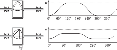
Figure 10.9. Shapes of constant width applied to cam design.

An alternative curve can be used that provides two dwells whose periods can be chosen to suit the application. It is based on the isosceles triangle shown in the right-hand column of figure 10.4 and has two dwells of (180 - 2t)° per revolution. This cam, with t = 45°, is shown in figure 10.9. Notice that while the displacement between dwells is less, the overall time spent in a dwell position amounts to 180°, i.e. half of the rotation. The actual displacement can be amplified by linkages of course. In practice, the actual cam shape of both curves would allow for the vertices to be rounded to reduce wear in the way shown in the first family of curves in figure 10.4.

A limiting form of cam operates in the ‘Scotch yoke’, or crank and slotted head, shown in figure 10.10(a). The curve here is a circle pivoted about the axis outside its perimeter, it is a true crank, and not a cam. The design lends itself to a compact form of engine suitable for use in steam pumps for boiler water feed. One end is the piston rod of the steam cylinder and the other is a piston rod from the pump, and the purpose of the crank is to drive a flywheel so that steam can be used expansively and so more economically. A similar yoke device was commonly used for foot wheels to drive watchmaker’s lathes before small electric motors were available. They are quiet, of variable speed and can be reversed at will. We have found them easy to use but have no experience of using such a lathe for long periods of time.

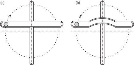
Figure 10.10. (a) The Scotch yoke and (b) the Scotch yoke with dwell.

The Scotch yoke is effectively a connecting rod of zero length with the result that as the crank turns it produces simple harmonic motion in the yoke. The same motion can be achieved with a connecting rod only if it is infinitely long. A modified yoke is shown in figure 10.10(b) that provides one dwell per revolution when the radius arc of the yoke equals that of the crank. In a sense this behaves like an inverted cam. The form of rectilinear motion is usually determined by the shape of the rotating cam, but here this motion is governed by the shape of the yoke.

An entirely different use for curves of constant width is as drills or milling cutters to form square holes. One design, which is easily identifiable as a square drill, was proposed by Harry James Watts in 1914. This employs a Reuleaux rotor in which three parts have been removed to provide the cutting edges and to allow the material removed to escape. A model is shown, together with the hole which it cuts, in plate 20. You will notice that it does not remove a perfect square and that small arcs remain in the corners.

The problem of rounded corners is overcome by again using the curve of constant width based on the isosceles triangle, shown on the right of figure 10.4. In particular we use the case with t = 45°. If a cam of this shape is housed in a square hole of side length w, then part of the quadrant from D to E must always touch one of the sides. Hence, the locus of the point C must follow a square path as the shape is rotated inside a square. A simple calculation reveals that the side length of this is w( - 1). In figure 10.11 we sketch the path of C for various orientations of the shape.

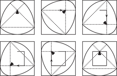
Figure 10.11. Cutting a square hole.

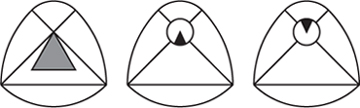
Figure 10.12. Details of a practical cutting tool for a square drill.

A real application of this curve was described in Mechanical World in 1939. The need was for a drill to cut blind holes, half an inch square and three-eighths of inch deep, in yellow brass. The cutting tool was a large equilateral triangle cutter.

An alternative form of cutter suitable for demonstration purposes only is shown in figure 10.12. A bar of round tool steel is ground off at one end to give a cutting edge on its centre line. This is held in a bore through the cam, centred at the intersection of the diagonals. The interest arises if the tool is turned through 180° so that the cutting edge faces inwards. Then the result is not a hole but a ‘square land’ of exactly the same size: of little practical use, perhaps, but it is fascinating to watch it being made. This drill is shown in plate 21, although unfortunately in this photograph the end of the cutting tool has sheared off during overzealous use.

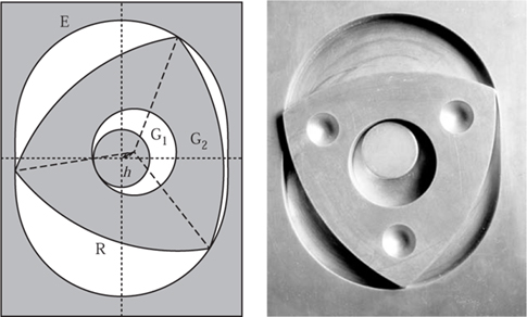
Figure 10.13. An application to engine design.

To use either drill in practice requires a pilot hole to be drilled first so that there is the minimum of material left to receive the final cuts. There is also the question of how to drive each drill, since the axis of any shaft cannot be fixed. The usual solution is to use a device known as an Oldham coupling. The flange at the end of the driving shaft, a fixed axis, is provided with a slot, as is the floating shaft connected to the cam. In between there is a disc with a bar either side, at right angles to the disc, that can slide in the slots. Incidentally, if the axis of the floating shaft is also fixed, a cutting tool in the plane of these axes will cut the disc to a true ellipse. This is the basis for the eccentric chuck frequently used in ornamental turning.

The final application of the Reuleaux rotor is in the design of the rotary-engine car. In a traditional engine the piston reciprocates but in a rotary engine, as the name implies, direct circular motion is generated. While full details of the engine itself can be found in Cole (1972), for example, for us the most interesting part is the geometry of the engine. With reference to figure 10.13 we take a Reuleaux rotor R and, from the centre, drill a large hole to create an internal gear of radius 3h. This gear is labelled G₂. This then rotates on a fixed gear of radius 2h, labelled G₁. If the distance from the centre of the rotor to the apex is 3r, then the width of the rotor is 6r cos(30°). Physical constraints determine the size of the Reuleaux rotor, relative to the gears. For example, it is necessary that the gears actually lie inside the Reuleaux rotor and this will occur if h < . By symmetry it is clear that the three vertices of the rotor all move along the same path. Taking R := 2r we can show that the path, E, is given by

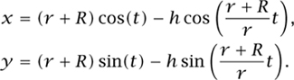
A model of this is shown in figure 10.13. The shape of this path is known as an epitrochoid, and to describe this further would take us too far from the topic of roundness to which this chapter is devoted. Its shape is described in Nash (1977) and for other related applications we highly recommend Holmes (1978).

10.5 Making Shapes of Constant Width

All curves of constant width are fascinating and can be cut from coloured plastic sheet or plywood easily enough. These can be made into rollers, or even used for decoration such as a mobile for a baby’s room. Making a cylinder of wood or metal with the cross-section of a Reuleaux rotor is a very different story. To make one of these cylinders requires careful and precise marking out of the stock material and equally precise positioning of the work in a lathe. It is not impossible but we felt it to be well beyond our capabilities and so we have not even tried to make one. Instead we make three simultaneously using a very simple method.

One of the readily available stock sections of bar metal is a true hexagon. Aluminium is a good choice, as is brass. While they are easy to turn with standard equipment, the method is not obvious and we feel that a little more detail is in order. The first task is to go over all faces with a perfectly smooth flat file to remove any tarnish and to highlight the edges, which must not be touched. Cut off three lengths and hold these in a three-jaw self-centring chuck with no more than 60–70 mm protruding to be turned. Turn down with the lathe until the cuts just reach the edges, and do it slowly with fine cuts because the cut is interrupted.

Remove the work from the chuck and check that the jaws have not bruised the metal, restoring the flatness if necessary. Next, rotate each piece through 120° and repeat the process, and then repeat a third time before parting off. The ends of each cylinder can then be faced off. You now have three identical rollers and you have been able to achieve this without any measurement. The results of this procedure are shown in plate 22.

If you are fortunate enough to have access to a CNC lathe, turning solids that have a cross-section of any piecewise circular curve of constant width with an axis of symmetry is straightforward. Once the tool shape is known, programming the lathe for circular arc profiles is usually quite simple. This is how the aluminium solids in plate 18 were produced. There will always be a pip at the end of the solid, formed when parting off, but it can be filed off without difficulty and without spoiling the shape. Larger wooden solids can be made on a conventional screw cutting lathe by careful measurement.

When you have made a solid and satisfied yourself that it is of constant width, be prepared for some scepticism and disbelief when you show it to others. The usual demonstration is to place the solid on a table and roll a hardback book on it. In some positions the centre of mass will be moving upwards and the very slight extra effort can be sensed and interpreted as poor workmanship on your part because the width is variable. In positions where the centre of mass is falling the false conclusion is still apparent to the sceptic. For this reason it is more convincing if the solid is made from a low-density material, like wood or aluminium, rather than from brass.

10.6 Roundness

We have seen that shapes of constant width, such as Reuleaux’s rotor, do have legitimate applications. However, more problematic are shapes with lobes which can crop up when manufacturing round parts. The production process may include imperfect machine tools that induce corresponding imperfections in the part being manufactured. In another situation, imagine holding a workpiece in a lathe using a three-jaw chuck. This work is compressed while it is turned, and when released the resulting shape may deform and hence deviate from roundness, even if it was manufactured to a high specification. If a workpiece is not sufficiently supported during turning, then it is possible to develop regular lobes. Another common engineering application in which lobes can develop is centreless grinding. In this process the workpiece is supported on a static blade between a high-speed grinding wheel and a slower-speed regulating wheel with a smaller diameter. Sometimes one or both wheels are aligned out of the horizontal plane. This imparts a horizontal velocity component to the work so that an additional feed mechanism is not necessary. There are advantages to centreless grinding, including shorter loading times. The workpiece is also being supported constantly, which makes it possible to either make heavier cuts or to grind shapes with a very small diameter. A normal lathe creates quite an axial load, which is absent in centreless grinding, and this is a crucial consideration for work that is easily distorted. The process allows automatic feeding and hence the continuous production of large quantities of small pieces. The simplicity of the machines cuts down maintenance costs. Despite these advantages, in centreless grinding a part is not held firmly and rotated on an axis. It is simply allowed to generate its own shape. Shapes of constant width can and do occur here. Hence, shapes with lobes do occur in manufacture and it is imperative to have practical tests that measure deviation from true roundness.

We often take improvements to manufacturing techniques for granted. It is only older readers who will remember seeing new cars with the instructions ‘running in, please pass’ in their rear windows. For the first 500 miles it was common practice to limit speed to 30 mph, and not to exceed 40 mph for the next 500 miles, before changing the oil. Improvements in the reproducibility and quality-control standards of the manufacture of rotating parts, in terms of roundness and surface finish, mean that a new car engine is effectively run-in as soon as it comes off the production line. It is as well to remember that car manufacture for most models is a mass production process.

Before we consider practical roundness tests in detail, we should mention two other aspects that are crucial to engineering practice. The first is surface texture and the second is cylindricity. Surface texture is concerned with the micro scale of the boundary of the shape, whereas we are most concerned here with the macro scale geometry. Of course, with very small departures from roundness and very large numbers of lobes on a surface it becomes impossible to form a clear distinction between the two. All manufactured objects are three dimensional, and hence one really makes a cylinder rather than a thin round disc. Since our interest in this chapter is the geometry of roundness of two-dimensional shapes, we shall concentrate exclusively on this and how we can measure departures from roundness. So, while the other two aspects cannot be ignored by a practical engineer we shall not comment further on them here.

When we describe a shape as ‘round’, we mean that the cross-section is circular, which is to say that all points are equidistant from the centre. Departure from roundness can be measured in a number of theoretical ways. The first is to find the maximum deviation from the minimum circumscribed circle. For example, if we carefully measure the width of a 20p piece, then the width is 0.844 in. However, a coin will not fit into a hole of this diameter. From our experiments, the minimum diameter hole into which a 20p piece will fit, i.e. the diameter of the minimum circumscribed circle, is 0.857 in. An experimental test block illustrating this is shown in figure 10.14. Despite appearances, the two holes have been machined to very high accuracy indeed, and an undamaged 20p piece only just fits into the bottom hole.

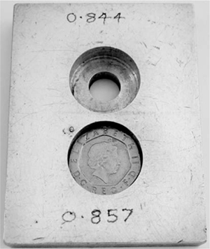
Figure 10.14. The minimum circumscribed circle of a 20p piece.

Similarly, we could measure the maximum deviation from the maximum inscribed circle. The least squares reference circle occurs where the area inside the shape but not the circle equals the area inside the circle but not the shape. Departure from roundness is the maximum deviation from this circle. Another measure that we will consider below is the minimum zone circle, which is defined as the minimum radial separation between two concentric circles positioned to enclose the shape. Note that only in special cases will the circumscribed and inscribed circles mentioned be those which give the minimum zone circle. All these are theoretical. An engineer needs some practical tests that can be applied in the workshop, from which these measures can be calculated.

10.7 The British Standard Summit Tests of BS3730

We have categorically seen that a shape that has constant width is not guaranteed to be a circle. What, then, can we measure to ascertain if a shape is circular, and how can we quantify any departure from roundness?

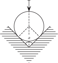
Figure 10.15. A circle in a vee-block.

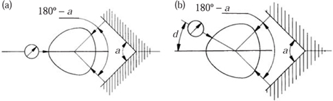
Figure 10.16. The British Standard summit methods: (a) symmetrical and (b) asymmetrical.

We want you to imagine a circle resting in a vee-block with an internal angle a, as shown in figure 10.15. By symmetry the top of the circle will be found on the angle bisector of the two faces of the vee-block. We shall constrain a measuring device so that it remains on this line. It is clear that if the shape is rotated in the vee-block then the position of the measuring device stays constant and, furthermore, that this is true no matter how big or small the angle is. Can we conclude the converse? That is to say, if a shape rotates smoothly inside a vee-block and the position of the measurer remains constant, is the shape round?

Measuring the width in various orientations can be thought of as a two-point measurement. In engineering practice the two-point measurement is supplemented by various three-point methods. Indeed, part 3 of the British Standard for ‘Assessment of departures from roundness’ (BS3730, 1987, British Standards Institute) is concerned with ‘Methods for determining departures from roundness using two- and three-point measurement’. BS3730 includes the so-called three-point summit method in symmetrical and asymmetrical settings: this is illustrated in figure 10.16. We will focus our attention on these tests. Other tests in the standard include the rider method, in which the workpiece rests in a vee-block and a measurement is taken between the vee-block and the workpiece. We do not consider these or methods for the measurement of internal surfaces, which are analogous.

The crucial question for us is the choice of angles a and d in the summit tests illustrated in figure 10.16. Quoting from BS3730 extensively:

In order to cover all possible form deviations and numbers of undulations always take one two-point measurement and two three-point measurements at different angles between fixed anvils. NOTE: The measurement procedures may, under certain preconditions, be amplified (see Table 2, Table 3 and Table 4). Select the angles between fixed anvils from the following:

• symmetrical setting: a = 90° and 120° or a = 72° and 108°;
• asymmetrical setting: a = 120°, d = 60°, or a = 60°, d = 30°;

where a is the angle between fixed anvils; d is the angle between the direction of measurement and bisector of angle between fixed anvils.

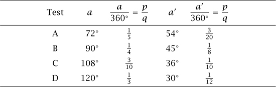
We shall consider six tests, the first four of which are the symmetrical summit tests. We supplement these with a symmetrical test using a vee-block with an angle of 60°, which, strictly speaking, is not in the British Standard, and then consider one of the asymmetrical tests, which results in a closed triangle. In this triangle we have internal angles 30°, 60° and 90°. Table 10.10 shows the angles for the symmetrical tests together with the angle a′ = (180° − a). This is the base angle in an isosceles triangle formed from the angle a. We have also listed these angles as fractions of 360°, which will prove to be important later.

Table 10.1. Angles in the BS3730 summit tests.

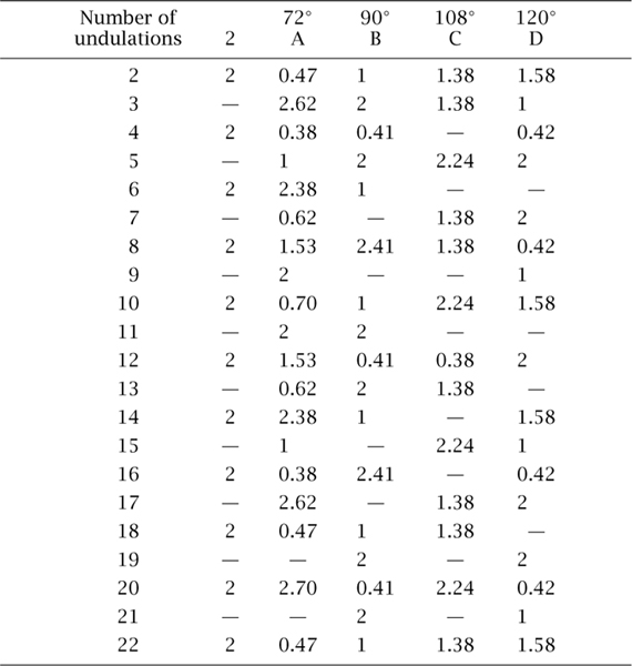
Some of the relevant data from the numbered tables in the standard that are quoted above are amalgamated in table 10.2. This table provides a correction factor, which we refer to as F, used in quantifying a departure from roundness for each of the tests A, B, C and D. Note that where the table shows a ‘—’ the use of the specific test is prohibited when this number of undulations is known. For example, the column labelled 2 refers to the two-point measurement, i.e. measuring the width. The data show that a width test should not be applied to an object with an odd number of undulations, which in the light of our previous discussion is a necessary precaution. To obtain a measured departure from roundness, the formula

δ = Δ/F

is used, where Δ is the largest measured departure from roundness for the tests applied. Of course, this all assumes that the number of undulations is known in advance.

We should note at the outset that this portion of the standard does not claim to provide methods which always work accurately.

The methods described in this Part of this standard may give faster and cheaper ways of assessing departures from roundness. This assessed value will deviate from the true value.

BS3730, p.4

Table 10.2. Correction factors for the British Standard summit tests (see text for details).

Instead of perfect mathematical accuracy, the aim is more pragmatic since the vee-block test requires only relatively simple workshop equipment.

10.8 Three-Point Tests

We have conducted practical experiments with a standard 90°vee-block. For example, in figure 10.18 we have a 50p being supported by a vee-block. The vee-block and the dial gauge are supported on a very accurate plane surface and the position of the dial gauge is moved to establish the maximum height of the workpiece above the plane surface. Note that this is quite a different procedure from fixing the vee-block and moving the dial gauge vertically along the angle bisector between the two fixed anvils, as would be the case in the tests specified in the British Standard.

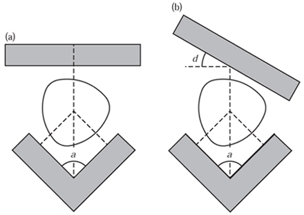
Figure 10.17. Three-point ‘summit’ methods: (a) symmetrical and (b) asymmetrical.

Our dial gauge measured vertical displacement to an accuracy of ± 0.01 mm. To this level of accuracy we could detect no difference between the point-up and point-down positions, or in any of a number of positions in between. Indeed, the deformations caused by everyday use, such as being dropped on one corner, were larger than the difference caused by position. Hence, according to the 90° vee-block alone a 50p was indistinguishable from a round object. We shall see in a moment that the geometry suggests that we might actually expect this to be the case. Indeed a 50p has seven undulations and looking at column B of table 10.2 tells us that the 90° vee-block should not be used in the British Standard tests either.

The Reuleaux rotor shown in plate 22 was quite a different story. This was made to have a width of approximately 25.4 mm (which is no accident), and the difference between the point-up and point-down positions is 7.98 ± 0.01 mm.

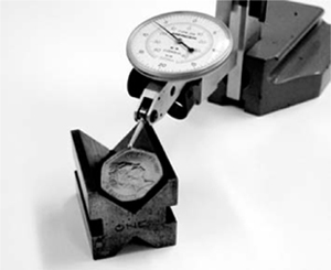
Figure 10.18. Applying the three-point summit method to a 50p piece with a 90° vee-block.

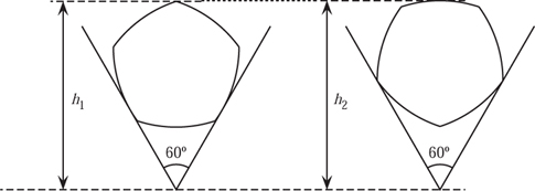
Figure 10.19. A circular arc rotor in a 60° vee-block.

We shall now use some trigonometry and apply this test to one of the circular arc rotors to illustrate the technique. This time we shall imagine a circular arc rotor generated from a regular pentagon sitting in a 60° vee-block. Two potential positions for this are shown in figure 10.19.

It is a straightforward exercise in trigonometry to show that if the width is 1, then h₁ = 1.497 246 and h₂ = 1.502 754, giving a difference of some 0.005 51 units, or 0.551%. Hence, this test indicates that the shape is not round. But do such tests always work? It certainly did not seem to work with a 50p in a 90° vee-block. That is to say, our experiment did not establish that a 50p is not round!

10.9 Shapes via an Envelope of Lines

To illustrate how the values in figure 10.17. In the symmetrical test shown in part (a), an anvil is lowered onto the workpiece and as contact is made the relative positions of the three anvils are measured. In the asymmetrical test (part (b)), the third anvil moves along a line at an angle.

It is important to note a subtle, but crucial, difference between the tests proposed in the British Standard and those that we are about to discuss. We consider the distances between three tangent lines. In the case of a non-smooth shape, such as Reuleaux’s rotor, these are support lines at fixed relative angles. In the British Standard summit tests there are two fixed anvils which, as before, operate as tangent lines. In the case of the symmetrical tests the measurement is taken by finding the points on the curve that lie on the angle bisector of these tangent lines. The point closest to the angle is the ‘rider point’, although we are most interested in that furthest away, which is the ‘summit point’ (see figure 10.16). We know nothing in particular about the direction of the tangent line at this point.

A shape of constant width can also be thought of as a rotor of the square. Indeed, this very property was used in both cam design and the square-hole drill, as demonstrated in plate 21. We are also interested in finding shapes of constant width that are also rotors of triangles. That is to say that the shape may be smoothly turned while remaining in contact with all three sides of a fixed triangle.

If, for example, we chose the angle a in the symmetrical vee-block to be 60°, we are led to consider the question, does there exist a shape with constant width which passes the 60° vee-block test? Such a shape would be a rotor of the square (constant width) and equilateral triangle (passes the 60° vee-block test). In fact we go further and explain how to construct a shape of constant width that rotates inside each member of a family of specified triangles. It will be clear that this shape is by no means unique, and that a whole family of such shapes exists.

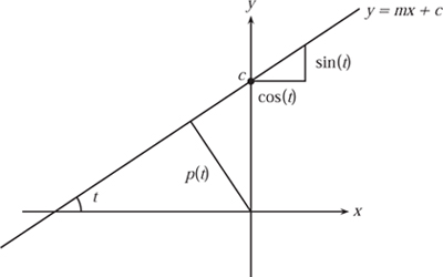
Figure 10.20. The equation of a straight line.

Let us begin with the usual equation for a line, y = mx + c. We shall assume that this line makes an angle t with the x-axis and that the perpendicular distance of the line from the origin is p = p(t). We prefer to make p depend on t, since in a moment we shall make extensive use of this. A diagram has been sketched in figure 10.20. Since m is the gradient of the line it follows that tan (t) = m, and simple trigonometry allows us to see that c = p(t)/ cos(t). Hence we can rewrite the equation of the line as y = tan(t)x + (p(t)/cos(t)), and this can in turn be recast in the form

This form of a straight line is more general since vertical lines can be represented when cos(t) = 0.

By giving a function for p(t) we shall generate a family of lines, and we denote a particular line by L_t. The region enclosed is known as the envelope and this will enable us to generate a variety of shapes. When we talk of a curve we refer to the boundary of this region. This method of constructing curves as the envelope of a series of tangents has already been used in figure 7.10 to define the parabola using the purely mechanical means of a pin, straight edge and square.

Indeed, if we revisit figure 7.10, it is clear that the equation of the tangent line AP is

y = x tan(t) − a tan (t),

so that in the form (10.1) we have

y cos(t) − x sin(t) = −a sin(t).

Hence, a parabola is generated by taking p(t) = −a sin(t). Another example of such an envelope of lines, showing a closed curve, is shown in figure 10.21.

For the purposes of this discussion we shall assume that t is measured in radians, so that an angle of 180° can more simply be written as π. Notice that by definition each line is tangent to the curve. Hence, to show that the curve has constant width it will be sufficient to consider the perpendicular distance between L_t and L_t+π, which are lines 180° apart, or rather parallels. In our case, the perpendicular distance between the two lines through the origin is simply p(t) + p(t + π).

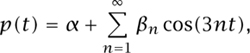
Here we will consider only envelopes generated by

Notice that if β = 0 then all lines are a constant distance from the origin, and the curve generated will be a circle of radius α. We do need to be careful, however, since if we take β to be too large, then the resulting shape is not a convex region of the plane: see, for example, figure 10.22.

Here the lines L_t and L_t+π will be parallel and a distance

2α + β cos(nt) + β cos (nt + nπ)

apart. Since n is an odd integer, cos(nt + nπ) = − cos(nt), so the lines are simply a distance 2α apart. Therefore, (10.2) automatically generates a shape of constant width.

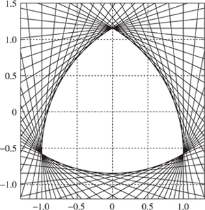
Figure 10.21. Reuleaux’s rotor via an envelope of lines.

If we think of (10.2) as adding an odd-frequency perturbation to the circle, we might generalize this and add more than one such perturbation. Hence we could generalize (10.2) to something like

It is even possible using an infinite sum to obtain an expression for Reuleaux’s rotor, which Kearsley (1952) gives as

where

A sketch of this is shown in figure 10.21. However, for us the generality of (10.3) adds nothing essentially new, and so here we consider only p(t) given by (10.2). Of course, we still need to establish that the resulting envelope is a convex region of the plane.

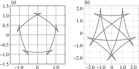
Figure 10.22. An example: n = 5 and α = 1, with (a) β , and (b) β =

An envelope of lines is a very simple way of defining a shape, and it is also invaluable to know the equations of these tangent lines when cutting such a shape with a CNC milling machine. However, the collection of lines does not provide us with an explicit mathematical expression for the shape itself.

To derive a direct parametric representation of the curve we consider the point of intersection of L_t and L_{t + ε}. For epsilon very close to zero the lines are practically coincident, and the point of intersection practically lies on the curve itself. Taking the limit as ε tends to zero will be a point on the curve itself. A calculation gives this, and substituting this back for the y-coordinate gives an explicit parametric form for the curve:

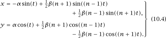
In this form it is clear that we have a circle of radius α to which two higher-frequency modes, with amplitudes proportional to β, have been added.

The parametric expression (10.4) allows us to derive straightforward criteria for when the envelope of lines generates a convex curve. This will occur if, and only if, there are no points of self-intersection of the curve. This is certainly satisfied if both x(t) and y(t) have at most two extremal values on the interval t ∈ [0, 2π). Again, a calculation gives the criterion that

Typically we shall assume that α = 1 and take β = 1/(n² − 1).

If we define r² = x² + y², then from (10.4) a further calculation gives

r² = α² + β²(n² + 1) + 2αβ cos(nt) − β²(n² − 1) cos(2 nt).

Taking t = 0 gives r²= (α + β)², and taking t = π/n gives r² = (α − β)²—these turn out to be the maximum and minimum values for r². Therefore,

Measuring the departure from roundness using the minimum zone circle, we have a value of 2β.

So, we have not only a method for cutting this family of shapes on a CNC machine but also an explicit mathematical expression for the curve given by (10.4) and we know the departure from roundness.

10.10 Rotors of Triangles with Rational Angles

So far we have generated a family of convex curves. Now we try to see how we can choose the parameters to create rotors of triangles. In this section we begin by considering an arbitrary triangle, such as ABC shown in figure 10.23. We denote the lengths of sides BC, AC and AB by l_a, l_b and l_c, respectively, and the perpendicular distances from the origin p_a, p_b and p_c. By the sine rule we have that, for some k,

Then sin(a) = kl_a, sin(b) = kl_a and sin(c) = kl_c, and

2k area(OBC) = p_a sin(a).

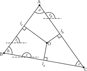
Figure 10.23. An arbitrary triangle.

Summing over the three triangles OBC, OAC and OAB gives

2k area(ABC) = p_a sin(a) + p_a sin(b) + p_c sin (c).

In addition, 2 area(ABC) = l_bl_c sin(a). Hence

2k area(ABC) = l_c sin(a) sin (b).

Combining these results we have that

p_a sin(a) + p_a sin(b) + p_a sin(c) = l_a sin(a) sin(b).

Take two similar triangles ABC and A′ B′ C′ in which l_a = λ , etc.

If

p_a sin(a) + p_b sin(b) + p_c sin(c)

then

l_c sin(a) sin(b) = l′_c sin(a) sin(b) = λl_c sin(a) sin (b),

so λ = 1 and hence ABC and A′ B′ C′ are identical.

With this result in mind we make the assumption that n ≠ 1 is an odd integer and define = n ± 1, which is a non-zero even integer. We assume that angles a, b and c are such that a, b and c are all integer multiples of 2π. If we take a family of lines (10.2), then provided α and β satisfy (10.5) the curve is convex. We now argue that the curve is indeed a rotor of the triangle ABC.

We construct the triangle ABC by taking the lines with the angles t_a = t, t_a = t − π + c and t_c = t + π − b. The triangles parametrized by t in this way will all be similar. We are required to show that they are identical, and hence the curve is indeed a rotor of the triangle ABC. To do this we note that a = π − b − c and consider

p(t) sin(a) + p(t_b) sin(b) + p(t_c) sin(c)

= α(sin(a) + sin(b) + sin(c))

+ β sin(π − b − c) cos(( − 1)t

+ β sin(b) cos(( − 1)(t − π + c))

+ β sin(c) cos(( − 1)(t + π − b)).

Omitting a lengthy calculation in which we use the assumptions that is a non-zero even integer and that b and c are multiples of 2π we arrive at

p(t) sin(a) + p(t_b) sin(b) + p(t_c) sin(c)

= α(sin(a) + sin(b) + sin(c)),

which is independent of t, and hence constant.

10.11 Examples of Rotors of Triangles

First we apply these results with the modest goal of designing a shape of constant width that is also a rotor of the equilateral triangle. All the angles in an equilateral triangle are 60°, or π/3. Hence, taking = 6 ensures that multiplied by each angle is equal to 2π. Hence n = 5 is sufficient in (10.2), although alternatively we could have taken n = 7. If we take α = 1 then (10.5) gives the largest possible β = , and each line in the envelope will be of the form

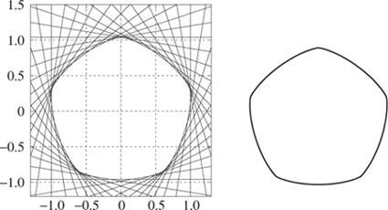
Figure 10.24. A rotor of both the square and the equilateral triangle.

An envelope of forty lines is shown on the left of figure 10.24, and its parametric expression

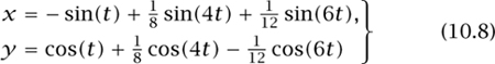
is plotted on the right. In this case, the width is 2 and a calculation shows that the lengths of the sides in the triangle are 2. Taking concentric circles with radii α ± β gives the departure from roundness (using the minimum zone circle measurement) of , or approximately 8.3%.

Next take a more general triangle in which all the angles are rational fractions of a rotation. That is to say, each angle a can be written as

Assume that for each angle in the triangle ¯n(p/q) is an integer. Let n be defined to be either + 1 or − 1. Assume further that the convexity constraint (10.5) is satisfied. Then the scheme (10.2) will generate a rotor of this triangle. Taking as the lowest common multiple of the denominators q suffices.

If we consider an isosceles right-angled triangle, this has two different angles 90° and 45° which can be expressed as a and an of a rotation. It is clear that taking = 8 ensures that (p/q) is an integer, and so n = 7 or n = 9 generates a rotor of the isosceles right-angled triangle.

If we want to create a shape that will be a rotor of more than one triangle, then we need to consider all the angles involved. For example, to find a shape that is simultaneously a rotor of the equilateral triangle and of the isosceles right-angled triangle, we now have three fractions to consider: 60° = , and . Taking = 24 and n = 23 suffices.

We might go even further and try to find a single shape that is a rotor of all the triangles with angles specified in table 10.1. We take as the lowest common multiple of the denominators of fractions ′ in this table. Hence = 8 × 3 × 5 = 120 suffices for the triangles generated by the angles in table 10.1. If we supplement these tests with a 60° vee-block, resulting in an equilateral triangle, then = ′ = 60° and /360° = . We refer to this as test E and in fact = 120 also generates a rotor of the equilateral triangle. More importantly, for the asymmetrical case a = 60° and d = 30° we generate a triangle with internal angles 60°, 90° and 30°, all of which are accounted for already. Hence, this asymmetrical summit test adds nothing essentially new to this geometric problem. The remaining asymmetrical test does not result in a triangle, and we do not consider it further.

Taking n = − 1 = 119 in (10.5) suggests that this generates a departure from roundness of about 2/(119² − 1) = , or 0.014%. This is too small for us to be able to provide an illustration, but it would be similar to that in figure 10.24 with 119 undulations.

If we choose the pairs of triangles that result from legitimate choices in the British Standard, then the first option for symmetrical settings is to apply tests B and D. Doing this results in fractional angles without a factor of 5 in the denominator. Hence = 24 suffices and consequently the departure from roundness is 0.38%. The second option for the symmetrical settings is to apply tests A and C. Any shape generated by (10.1) which is a rotor of the triangle with angles specified by test A is automatically a rotor of the triangle with angles from test C, and so from our point of view this test contributes nothing and = 20 suffices, giving the departure from roundness as 0.56%.

If we return to our experiment with the 50p piece then we have a shape with 7 undulations—again it makes little sense to apply test B, as we did in figure 10.18. With = 8, the test ignores n = 7 undulations. Interestingly, if we consider test A from table 10.1, then = 20 is the smallest value and our related geometric analysis would suggest that we should beware of using this test with n = ± 1, i.e. 19 or 21 undulations. Indeed, these are precisely the numbers of undulations for which the British Standard summit test A should not be used. For test B, = 8. Here we need to consider n = k ± 1 for k = 1, 2,..., since after all we only require (p/q) to be an integer for each angle in the test. Thus we should avoid this test for shapes with 7, 9, 15 or 17 undulations. Although our tests are not those specified in the British Standard, the geometry we have examined goes some way to explaining how table 10.2 might be derived.

One might imagine that by applying the two-point measurement method and then a number of different three-point techniques we could be confident that the shape was round. Indeed, Reason (1966, p. 17) claims the following.

If several V-block determinations are recorded each with a different angle, it should be possible, with an electronic computer, to find the true shape of the part from the combined results, the principle being that there can only be one set of radial measurements that will account simultaneously for all the V-block measurements.

Our method allows us to create a rotor for a whole family of triangles. Hence, it seems that Reason’s principle provides very shaky foundations indeed, especially when a finite number of vee-blocks are used. It appears that from a purely theoretical point of view our vee-block tests are little better than width measurement.

No matter how many different tests we propose applying, provided all the angles are rational, we can construct a single shape which is a rotor of them all. However, our test involving a triangle with some irrational angles cannot be accommodated within this scheme. Indeed, a remarkable theorem of Kamenet-ski (1947) applied to triangles proves that necessary and sufficient conditions for the existence of a rotor of a triangle are that all angles are rational. Thus, a single irrational triangle has no rotors, and hence would provide a sufficient three-point summit test for roundness. While constructing an irrational-angled triangle might not be practical for the engineer, using fractional denominators that have a large lowest common multiple would result in a much greater and hence less deviation from roundness.

It is precisely this approach that is rather cleverly adopted by Goho, Kimiyuki and Hayashi (1999). They propose an angle of 14° = . In a symmetrical summit test the other two angles in this triangle are (180° − 14°) = 83°. Since 83 is prime, 83/360° cannot be simplified and we would need to take = 360, giving n = 359. With α = 1, the convexity constraint of (10.5) gives

Hence the departure from roundness is , or approximately 0.0015%, which is rather small. Furthermore, while we have chosen frequency modes in (10.2) in such a way that peaks and troughs cancel out so that there is no apparent difference in height of the dial gauge, other modes are actually amplified by rotation in a vee-block. This is shown in table 10.2, in which the F factors are greater that one. When the angle a is 14°, this can be by a factor of about nine. The practical engineer might well be happy knowing that some very-high-frequency modes, which result in small-amplitude departures from roundness, are ignored if the larger lower-frequency modes are amplified.

10.12 Modern and Accurate Roundness Methods

To complete this chapter we will very briefly describe how roundness is determined. We have comprehensively shown that simple vee-block methods do not provide reliable tests. One intuitive reason for this is that three points of contact contribute to the measured value in each position. This provides the opportunity for lobes to generate peaks and troughs that cancel each other out. Indeed, by considering regular lobes it is possible to derive an intuitive notion of when the three-point measurement is likely to give misleading results. While an irrational-angled triangle might be made to work, a much more direct method is to establish the position of the edge of the shape with a single point of contact.

We should recall that a round shape has a circular cross-section, and hence all points on the edge are equidistant from an axis of rotation. To determine roundness accurately a machine incorporates a turntable to rotate the object about a reference axis. This axis is independent of the part being measured. Some kind of measuring device, in the form of a stylus, then presses against the surface as the object rotates and a transducer converts the motion of the stylus into positional information. Typically a system will use 3600 points or more.

However, there are real practical difficulties in setting up the machine prior to such a measurement being taken. The first is the problem of centring. Consider, for example, measuring a sphere rotated about an axis that does not pass through the centre of the sphere. The next problem is levelling. To illustrate this consider measuring a perfect cylinder that has been tilted. A plane section is basically elliptical. Furthermore, if the stylus tip has a finite size, then the contact point also moves up and down the cylinder as it is rotated. This further distorts the measured shape—a problem known as cresting. Here, the projected line of action of the gauge does not pass through the axis of rotation. While cresting can be eliminated by correctly setting up the stylus, centring and levelling need to be performed for each measurement.

Modern machines can automatically move the object into position and establish the position and orientation of the object’s axis. They will then determine the departure from roundness using this axis. Such machines incorporate a large number of moving parts, all of which must be machined to the very highest specifications if imperfections in their manufacture are not to induce corresponding imperfections in the departure-from-roundness measurements being taken. These moving parts, the software needed to control such machines, and the calibration all combine. Highly expensive specialist equipment is the result. This complexity is necessitated by the geometry we have explained in this chapter.