Given two corresponding images taken with different lighting conditions, a unique solution can be obtained for the surface orientation at each point.

Example 3.4 Illustration of photometric stereo.

Two images of a sphere, taken with different lighting conditions (the same source has been put in two different position), are shown in Figure 3.12(a) and Figure 3.12(b), respectively. The surface orientation determined by photometric stereo is shown in Figure 3.12(c) by using an orientation-vector representation (the vector is represented by a line segment). It can be seen that the surface orientation is perpendicular to the paper in places closest to the center of the sphere, while the surface orientation is parallel to the paper in places closest to the edges of the sphere.

The reflectance properties of a surface at different places can be different. A simple example is that the irradiance is the product of a reflectance factor (between 0 and 1) and some functions of orientation. Suppose that a surface, which is like a Lambertian surface except that it does not reflect the entire incident light, is considered. Its brightness is represented by ρ cos θi, where ρ is the reflectance factor. To recover the reflectance factor and the gradient (p, q), three images are required.

Introducing the unit vectors in the directions of three source positions, it has

$S_j=\frac{{[-p_j-q_{j}1]}^T}{\sqrt{1+p_j^2+q_j^2}}j=1,2,3(3.33)$

Then the irradiance is

$E_j=\rho (S_j•N)j=1,2,3(3.34)$

where

$N=\frac{{[-p-q1]}^{\text{T}}}{\sqrt{1+p^2+q^2}}(3.35)$

is the unit surface normal. For unit vectors N and ρ, three equations can be obtained

$E_1=\rho (S_1•\text{N})E_2=\rho (S_2•N)E_3=\rho (S_3•N)(3.36)$

Combining these equations gives

$E=\rho S•N(3.37)$

where the rows of the matrix S are the source directions S1, S2, S3, and the components of the vector E are the three brightness measurements. Suppose that S is non-singular. It can be shown that

$\rho N=S^{-1}•E=\frac{1}{[S_1•(S_2\times S_3)]}[E_1(S_2\times S_3)+E_2(S_3\times S_2)+E_3(S_1\times S_2)](3.38)$

The direction of the surface normal is the result of multiplying a constant with a linear combination of the three vectors, each of which is perpendicular to the directions of the two light sources. If multiplying the brightness obtained when the third source is used with each of these vectors, the reflectance factor ρ will be recovered by finding the magnitude of the resulting vector.

Example 3.5 Recover the reflectance factor by three images.

Suppose that a source has been put in three places (–3.4, –0.8, –1.0), (0.0, 0.0, –1.0), (–4.7, –3.9, –1.0), and then three images are captured. Three equations can be established and the surface orientation and reflectance factor can be determined. Figure 3.13(a) shows three reflectance property curves. It is seen from Figure 3.13(b) that when ρ = 0.8, three curves are joined at p = –1.0, q = –1.0.

3.2Structure from Motion

The structure of a scene consisting of a number of objects or an object consisting of several parts can be recovered from the motion of objects in a scene or the different motion of object parts.

3.2.1Optical Flow and Motion Field

Motion can be represented by a motion field, which is composed of motion vectors of the image points.

Example 3.6 Computation of a motion field.

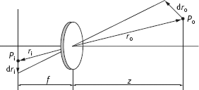
Suppose that in a particular moment, one point Pi in an image is mapped from a point Po at the object surface, as shown in Figure 3.14. These two points are connected by the projection equation. Let Po have a velocity Vo relative to the camera. It induces a motion Vi in the corresponding Pi. The two velocities are

$V_{\text{o}}=\frac{\text{d}{r}_{\text{o}}}{\text{d}t}{V}_1=\frac{\text{d}{r}_1}{\text{d}t}(3.39)$

where ro and ri are related by

$\frac{1}{\lambda }{r}_1=\frac{1}{r_{\text{o}}•z}{r}_{\text{o}}(3.40)$

where λ is the focal length of the camera and z is the distance (vector) from the center of the camera to the object.

According to visual psychology, when there is relative motion between an observer and an object, optical patterns on the surface of object provide the motion and structure information of the object to the observer. Optical flow is the apparent motion of the optical patterns. Three factors are important in optical flow: Motion or velocity field, which is the necessary condition of optical flow; optical patterns, which can carry information; and a projection from the scene to the image, which make it observable.

Optical flow and motion fields are closely related but different. When there is optical flow, certain motion must exist. However, when there is some motion, the optical flow may not appear.

Example 3.7 The difference between the motion field and optical flow.

Figure 3.15(a) shows a sphere with the homogeneous reflectance property rotating in front of a camera. The light source is fixed. There are brightness variations in different parts of the surface image; however, the brightness variations are not changed with the rotation of sphere, so the image is not changed in gray-level values with time. In this case, though the motion field is not zero, the optical flow is zero everywhere. In Figure 3.15(b), a fixed sphere is illuminated by moving the light source. The gray-level values in different locations of the image change as the illumination changes according to the source motion. In this case, the optical flow is not zero but the motion field of sphere is zero everywhere. This motion is called the apparent motion.

3.2.2Solution to Optical Flow Constraint Equation

The optical flow constraint equation is also called the image flow constraint equation. Denote f(x, y, t) as the gray-level value of an image point (x, y) at time t, u(x, y) and v(x, y) as the horizontal and vertical velocities of the image point (x, y), respectively. The optical flow constraint equation can be written as

$f_{x}u+f_{y}v+f_t=0(3.41)$

where fx, fy, ft are the gray-level gradients along X, Y, T directions, respectively.

In addition, eq. (3.41) can also be written as

$(f_x,f_y)•(u,v)=-f_t(3.42)$

3.2.2.1Computation of Optical Flow: Rigid Body

Equation (3.41) is a linear constraint equation about velocity components u and v. In the velocity space, as shown in Figure 3.16, values of u and v satisfying eq. (3.41) lie on a line,

$u_0=-f_t/f_x{v}_0=-f_t/f_y\theta =\text{arctan}(f_x/f_y)(3.43)$

All points on this line are the solutions of the optical flow constraint equation. In other words, one equation cannot uniquely determine the two variables u and v.

To determine uniquely the two variables u and v, another constraint should be introduced. When dealing with rigid bodies, it is implied that all neighboring points have the same optical velocity. In other words, the change rate of the optical flow is zero, which are given by

${(\nabla u)}^2={\left(\frac{\partial u}{\partial x}+\frac{\partial u}{\partial y}\right)}^2=0(3.44)$

${(\nabla v)}^2={\left(\frac{\partial v}{\partial x}+\frac{\partial v}{\partial y}\right)}^2=0(3.45)$

Combining these two equations with the optical flow constraint equation, the optical flow can be calculated by solving a minimum problem as

$\epsilon (x,y)={\displaystyle \sum _x{\displaystyle \sum _y\left\{{(f_{x}u+f_{y}v+f_t)}^2+{\lambda }^2[{(\nabla u)}^2+{(\nabla v)}^2]\right\}}(3.46)}$

In eq. (3.46), the value of λ depends on the noise in the image. When the noise is strong, λ must be larger. To minimize the error in eq. (3.46), calculating the derivatives of u and v, and letting the results equal to zero, yields

$f_x^{2}u+f_x{f}_{y}v=-{\lambda }^2\nabla u-f_x{f}_t(3.47)$

$f_x^{2}v+f_x{f}_{y}u=-{\lambda }^2\nabla v-f_y{f}_t(3.48)$

The above two equations are also called Euler equations. Let $\overline{u}\text{and}\overline{v}$ be the average values in the neighborhood of u and v, and let $\nabla u=u-\overline{u}\text{and}\nabla v=v-\overline{v}.$ Equation (3.47) and eq. (3.48) become

$(f_x^2+{\lambda }^2)u+f_x{f}_{y}v={\lambda }^2\overline{u}-f_x{f}_t(3.49)$

$(f_y^2+{\lambda }^2)v+f_x{f}_{y}u={\lambda }^2\overline{v}-f_y{f}_t.(3.50)$

The solutions for eq. (3.49) and eq. (3.50) are

$u=\overline{u}-\frac{f_x[f_x\overline{u}+f_y\overline{v}+f_t]}{{\lambda }^2+f_x^2+f_y^2}(3.51)$

$v=\overline{v}-\frac{f_y[f_x\overline{u}+f_y\overline{v}+f_t]}{{\lambda }^2+f_x^2+f_y^2}.(3.52)$

Equation (3.51) and eq. (3.52) provide the basis for solving u(x, y) and v(x, y) with an iterative method. In practice, the following relaxation iterative equations are used

$u^{(n+1)}={\overline{u}}^{(n)}-\frac{f_x[f_x{\overline{u}}^{(n)}+f_y{\overline{v}}^{(n)}+f_t]}{{\lambda }^2+f_x^2+f_y^2}(3.53)$

$v^{(n+1)}={\overline{v}}^{(n)}-\frac{f_y[f_x{\overline{u}}^{(n)}+f_y{\overline{v}}^{(n)}+f_t]}{{\lambda }^2+f_x^2+f_y^2}.(3.54)$

The initial values can be u(0) = 0, v(0) = 0 (a line passing through the origin). Equations (3.53) and (3.54) have a simple geometric explanation: The iterative value at a new point (u, v) equals to the difference of the average value in the neighborhood of this point and an adjust value that is in the direction of the brightness gradient, as shown in Figure 3.17.

Example 3.8 Real example of the optical flow detection.

Some results for a real detection of optical flow are shown in Figure 3.18. Figure 3.18(a) is an image of a soccer ball. Figure 3.18(b) is the image obtained by rotating Figure 3.18(a) around the vertical axis. Figure 3.18(c) is the image obtained by rotating Figure 3.18(a) clockwise around the viewing axis. Figure 3.18(d, e) are the detected optical flow in the above two cases, respectively.

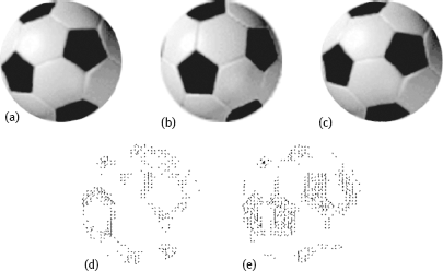
It can be seen from Figure 3.18 that the optical flow has bigger values at the boundaries between the white and black regions as the gray-level values change is acute there, and has smaller values at the inside place of the white and black regions as the gray-level values there show almost no change during the movement.

3.2.2.2Computation of Optical Flow: Smooth Motion

Another method for introducing more constraints is to use the property that the motion is smooth in the field. It is then possible to minimize a measure of the departure from smoothness by

$e_{\text{s}}={\displaystyle \iint [(u_x^2+u_y^2)+(v_x^2+v_y^2)]\text{d}x\text{d}y(3.55)}$

In addition, the error in the optical flow constraint equation

$e_{\text{c}}={\displaystyle \iint {[E_{x}u+E_{y}v+E_t]}^2\text{d}x\text{d}y(3.56)}$

should also be small. Overall, the function to be minimized is es + λec, where λ is a weight. With strong noise, λ should take a small value.

3.2.2.3Computation of Optical Flow: Gray-Level Break

Consider Figure 3.19(a), where XY is an image plane, I is the gray-level axis, and an object moves along the X direction with a velocity of (u, v). At time t0, the gray-level value at point P0 is I0 and the gray-level value at point Pd is Id. At time t0 + dt, the gray-level value at P0 is moved to Pd and this forms the optical flow. Between P0 and Pd, there is a gray-level break.

Considering Figure 3.19(b), look at the change of gray-level along the path. As the gray-level value at Pd is the gray-level value at P0 plus the gray-level difference between P0 and Pd, it has

$I_{\text{d}}={\displaystyle \underset{P_0}{\overset{P_{\text{d}}}{\int }}\nabla f•\text{d}l+I_0}(3.57)$

On the other hand, look at the change of gray level along the time axis. As the gray-level value observed at Pd is changed from Id to I0, it has

$I_0={\displaystyle \underset{t_0}{\overset{t_0+\text{d}t}{\int }}{f}_t\text{d}t+I_{\text{d}}}(3.58)$

The changes of gray-level values in the above two cases are equal, so combining eqs (3.57) and (3.58) gives

${\displaystyle \underset{P_0}{\overset{P_{\text{d}}}{\int }}\nabla f•\text{d}l}=-{\displaystyle \underset{t_0}{\overset{t_0+\text{d}t}{\int }}{f}_t\text{d}t}(3.59)$

Substituting dl = [u v]Tdt into eq. (3.59) yields

$f_{x}u+f_{y}v+f_t=0(3.60)$

Now it is clear that the optical flow constraint equation can be used when there is a gray-level break.

3.2.3Optical Flow and Surface Orientation

Consider an observer-centered coordinate system XYZ (the observer is located at the origin), and suppose that the observer has a spherical retina, so the world can be projected onto a unit image sphere. Any point in this image sphere can also be represented by a longitude ϕ, a latitude θ and a distance from the origin r.

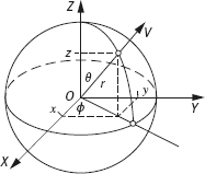
The above two coordinate systems are depicted in Figure 3.20, and can be interchanged.

$x=r\sin \theta \cos \varphi (3.61)$

$y=r\sin \theta \sin \varphi (3.62)$

$z=r\cos \theta (3.63)$

$r=\sqrt{x^2+y^2+z^2}(3.64)$

$\theta =\arccos (z/r)(3.65)$

$\phi =\arccos (y/x)(3.66)$

The optical flow of an object point can be determined as follows. Let the velocity of the point be (u, v, w) = (dx/dt, dy/dt, dz/dt), and the angular velocities of the image point in ϕ and θ (directions are

$\delta =\frac{v\cos \varphi -u\sin \varphi }{r\sin \theta }(3.67)$

$\epsilon =\frac{(ur\sin \theta \cos \varphi +vr\sin \theta \sin \varphi +wr\cos \theta )\cos \theta -rw}{r^2\sin \theta }(3.68)$

Equations (3.67) and (3.68) are the general expressions for the optical flow in ϕ and θ directions. Consider a simple example. Suppose that the object is stationary and the observer is traveling along the Z-axis with a speed S. In this case, u = 0, v = 0, and w = −S. Taking them into eq. (3.67) and eq. (3.68) yields

$\delta =0(3.69)$

$\epsilon =S\sin \theta /r(3.70)$

Based on eq. (3.69) and eq. (3.70), the surface orientation can be determined. Suppose that R is a point in the patch on the surface and an observer located at O is looking at this patch along the viewing line OR as in Figure 3.21(a). Let the normal vector of the patch be N . N can be decomposed into two orthogonal directions. One is in the ZR plane and has an angle σ with OR as in Figure 3.21(b). Another is in the plane perpendicular to the ZR plane (so is parallel to the XY plane) and has an angle τ with OR′ (see Figure 3.21(c), the Z-axis is pointed outward from paper).

In Figure 3.21(b), ϕ is a constant, while in Figure 3.21(c), θ is a constant. Consider σ in the ZR plane, as shown in Figure 3.22(a). If θ is given an infinitesimal increment Δθ, the change of r is Δr. Drawing an auxiliary line ρ, from one side, it gets ρ/r = tan(Δθ) ≈ Δθ, from other side, it has ρ/Δr = tan σ. Combining them yields

$r\Delta \theta =\Delta r\text{tan}\sigma (3.71)$

Similarly, consider τ in the plane perpendicular to the ZR plane, as shown in Figure 3.22(b). If giving ϕ an infinitesimal increment Δϕ, the change of r is Δr. Drawing an auxiliary line p, from one side, it has ρ/r = tan(Δϕ) ≈ Δϕ, and from the other side, it has ρ/Δr = tan τ. Combining them yields

$r\Delta \varphi =\Delta r\tan \tau (3.72)$

Taking the limit values of eq. (3.71) and eq. (3.72) yields

$\cot \sigma =\left[\frac{1}{r}\right]\frac{\partial r}{\partial \theta }(3.73)$

$\cot \tau =\left[\frac{1}{r}\right]\frac{\partial r}{\partial \varphi }(3.74)$

in which r can be determined from eq. (3.64). Since ε is the function of both ϕ and θ, eq. (3.70) can be written as

$r=\frac{S\sin \theta }{\epsilon \left(\varphi ,\theta \right)}\left(3.75\right)$

Taking partial differentiations of ϕ and θ yields

$\frac{\partial r}{\partial \phi }=S\sin \theta \frac{-1\partial \epsilon }{{\epsilon }^2\partial \phi }\left(3.76\right)$

$\frac{\partial r}{\partial \theta }=S\left(\frac{\cos \theta }{\epsilon }-\frac{\sin \theta }{{\epsilon }^2}\frac{\partial \epsilon }{\partial \theta }\right)\left(3.77\right)$

Substituting Eqs (3.65) and (3.66) into eqs (3.73) and (3.74) yields

$\sigma =\mathrm{arccot}\left[\cot \theta -\frac{\partial \left(\ln \epsilon \right)}{\partial \theta }\right]\left(3.78\right)$

$\tau =\mathrm{arccot}\left[\frac{\partial \left(\ln \epsilon \right)}{\partial \varphi }\right]\left(3.79\right)$