7Content-Based Image Retrieval

With the development of electronic devices and computer technology, a large number of images and video sequences (in general, a group of images) have been acquired, stored, and transmitted. As huge image databases are built, the searching for required information becomes complicated. Though a keyword index is available, it has to be created by human operators and it could not fully describe the content of images. An advanced type of technique, called content-based image retrieval (CBIR), has been developed for this reason.

The sections of this chapter are arranged as follows:

Section 7.1 introduces the matching techniques and similarity criteria for image retrieval based on color, texture, and shape features.

Section 7.2 analyzes the video retrieval techniques based on motion characteristics (including global motion features and local motion features).

Section 7.3 presents a multilayer description model, including original image layer, meaningful region layer, visual perception layer, and object layer, for object-based high-level image retrieval.

Section 7.4 discusses the particular methods for the analysis and retrieval of three types of video programs (news video, sports video, and home video).

7.1Feature-Based Image Retrieval

A typical database querying form is the query by example. Variations include composing multiple images or drawing sketches to obtain examples. Example images are described by appropriate features and are matched to the features of database images. The popularly used features are color, texture, and shape. Some other examples are the spatial relationship between objects and the structures of objects (Zhang, 2003b).

7.1.1Color Features

Color is an important feature in describing the content of images. Many retrieval methods are based on color features (Niblack, 1998; Zhang, 1998b; Zhang, 1998c). Commonly used color spaces include RGB and HSI spaces. In the following, the discussion is based on RGB space, although the HSI space is often better. Many color-based techniques use histograms to describe an image. The histogram of an image is a 1-D function

$\text{H}\left(\text{k}\right)=n_k/nk=0,1,\cdot \cdot \cdot ,L-1\left(7.1\right)$

where k is the index of the feature bins of the image, L is the number of bins, nk is the number of pixels within feature bin k, and n is the total number of pixel in an image.

In content-based image retrieval, the matching technique plays an important role. With histograms, the matching of images can be made by computing different distances between histograms.

7.1.1.1Histogram Intersection

Let HQ(k) and HD(k) be histograms of a query image Q and a database image D, respectively, and the matching score of the histogram intersection between the two images is given by Swain (1991)

$\text{P}\left(\text{Q,D}\right)=\frac{{\displaystyle \sum _{k-0}^{L-1}\min \left[{\text{H}}_{\text{Q}}\left(k\right),{\text{H}}_{\text{D}}\left(k\right)\right]}}{{\displaystyle \sum _{k-0}^{L-1}{\text{H}}_{\text{Q}}\left(k\right)}}\left(7.2\right)$

7.1.1.2Histogram Distance

To reduce computation, the color information in an image can be approximated roughly by the mean of histograms. For RGB components, the feature vector for matching is

$\mathit{f}={\left[{\mu }_R{\mu }_G{\mu }_B\right]}^T\left(7.3\right)$

The matching score of the histogram distance between two images is

$\text{P}\left(\text{Q,D}\right)=\sqrt{{\left({\mathit{f}}_{\text{Q}}-{\mathit{f}}_D\right)}^2}=\sqrt{{\displaystyle {\sum }_{R,G,B}{\left({\mu }_{\text{Q}}-{\mu }_D\right)}^2}}\left(7.4\right)$

7.1.1.3Central Moment

Mean is the first-order moment of histograms, and higher-order moments can also be used. Denote the i-th (i ≤ 3) central moments of RGB components of a query image Q by $M_{QR}^l,M_{QG}^l,\text{and}{M}_{QB}^l,$ respectively. Denote the i-th (i ≤ 3) central moments of RGB components of database image D by $M_{DR}^l,M_{dG}^l,\text{and}{M}_{DB}^l,$ respectively. The matching score between two images is

$\text{P}\left(\text{Q,D}\right)=\sqrt{W_R{\displaystyle \sum _{l-1}^3{\left(M_{\text{Q}R}^l-M_{DR}^l\right)}^2+W_G{\displaystyle \sum _{l-1}^3{\left(M_{\text{Q}G}^l-M_{DG}^l\right)}^2+}}{W}_B{\displaystyle \sum _{l-1}^3{\left(M_{\text{Q}B}^l-M_{DB}^l\right)}^2+}}\left(7.5\right)$

where WR, WG, and WB are weights.

7.1.1.4Reference Color Tables

Histogram distance is too rough for matching while histogram intersection needs a lot of computation. A good trade-off is to represent image colors by a group of reference colors (Mehtre, 1995). Since the number of reference colors is less than that of the original image, the computation can be reduced. The feature vectors to be matched are

$\mathit{f}={\left[r_1{r}_2{r}_N\right]}^T\left(7.6\right)$

where ri is the frequency of the i-th color and, N is the size of the reference color table. The matching value between two images is

$\text{P}\left(\text{Q,D}\right)=W\sqrt{{\left({\mathit{f}}_{\text{Q}}-{\mathit{f}}_{\text{D}}\right)}^2}=\sqrt{{\displaystyle \sum _{i-1}^N{W}_i{\left(r_{i\text{Q}}-r_{i\text{D}}\right)}^2}}\left(7.7\right)$

where

$w_i=\{\begin{array}{l}{r}_{i\text{Q}}{r}_{i\text{Q}}>0\text{and}{r}_{i\text{D}}>0\\ 1r_{i\text{Q}}=0\text{or}{r}_{i\text{D}}=0\end{array}\left(7.8\right)$

In the above four methods, the last three methods are simplifications of the first one with respect to computation. However, histogram intersection has another problem. When the feature in an image cannot take all values, some zero-valued bins may occur. These zero-valued bins have influence on intersection, so the matching value computed from eq. (7.2) does not correctly reflect the color differnce between the two images. To solve this problem, the cumulative histogram can be used (Zhang, 1998c). A cumulative histogram of an image is a 1-D function, given by

$I\left(k\right)={\displaystyle \sum _{i-0}^k\frac{n_i}{n}}k=0,1,\mathrm{...},L-1\left(7.9\right)$

The meanings of the parameters are the same as that in eq. (7.1). Using the cumulative histogram could reduce zero-valued bins; therefore, the distance between two colors is propotional to their similarity. Further improvement can be made by using the subrange cumulative histogram (Zhang, 1998c).

7.1.2Texture Features

Texture is also an important feature in describing the content of an image (see also Chapter 5 of Volume II in this book set). For example, one method using the texture feature to search a JPEG image is proposed Huang (2003).

One effective method for extracting texture is based on the cooccurence matrix. From the co-occurence matrix M, different texture descriptors can be computed.

7.1.2.1Contrast

$G={\displaystyle \sum _h{\displaystyle \sum _k{\left(h-k\right)}^2}{m}_{hk}}\left(7.10\right)$

For rough texture, the values of mhk are concentrated in the diagonal elements. The value of (h − k) would be small and the value of G is also small. Otherwise, for fine textures, the value of G would be big.

7.1.2.2Energy

$J={\displaystyle \sum _h{\displaystyle \sum _k{\left(m_{hk}\right)}^2}}\left(7.11\right)$

When the values of mhk are concentrated in diagonal elements, the value of J would be big.

7.1.2.3Entropy

$S=-{\displaystyle \sum _h{\displaystyle \sum _k{m}_{hk}\log m_{hk},\left(7.12\right)}}$

When the values of mhk in the cooccurence matrix are similar and are distributed around the matrix, the value of S would be big.

7.1.2.4Correlation

$C=\frac{{\displaystyle \sum _h{\displaystyle \sum _{k}hk{m}_{hk}-{\mu }_h{\mu }_k}}}{{\sigma }_h{\sigma }_k}\left(7.13\right)$

where µh, µk, σh, and σk are the mean values and standard variances of mh and mk, respectively. Note that $m_h={\displaystyle {\sum }_k{m}_{hk}}$ is the sum of the row elements of M, and mk = ${\displaystyle {\sum }_h{m}_{hk}}$ is the sum of column elements of M.

The size of the cooccurence matrix is related to the number of gray levels of the image. Suppose the number of gray levels of the image is N, then the size of the cooccurence matrix is N × N, and the matrix can be denoted M(Δx, Δy), (h, k). First, the co-occurence matrices for four directions, M(1,0), M(0,1), M(1,1), M(1,–1), are computed. The above four texture descriptors are then obtained. Using their mean values and standard deviations, a texture feature vector with eight components is obtained.

Since the physical meaning and value range of these components are different, a normalization process should be performed to make all components have the same weights.

Gaussian normalization is a commonly used normalization method Ortega (1997). Denote an N-D feature vector as F = [f1f2 ... fN]. If database images are denoted I1, I2, ..., IM, for each Ii, its corresponding feature vector is Fi = [fi,1 fi,2 ... fi,N]. Suppose that [f1,,j,f2,j ··· fi,j ··· fM,j] satisfies the Gaussian distribution, after obtaining the mean value mj and standard deviation σj, fi,j can be normalized into [-1,1] by

$f_{\text{i,j}}^{\left(\text{N}\right)}=\frac{f_{\text{i,j}}-m_j}{{\sigma }_j}\left(7.14\right)$

The distribution of $f_{l,j}^{\left(N\right)}$ is now an N(0,1) distribution.

7.1.3Shape Features

Shape is also an important feature in describing the content of images (see also Chapter 6 of Volume II in this book set). A number of shape description methods have been proposed (Zhang, 2003b). Some typically used methods are geometric parameters (Scassellati, 1994; Niblack, 1998), invariant moments (Mehtre, 1997), boundary direction histogram (Jain, 1996), and important wavelet coefficients (Jacobs, 1995).

7.1.3.1MPEG-7 Adopted Shape Descriptors

MPEG-7 is an ISO/IEC standard developed by MPEG (Moving Picture Experts Group), which was formally named “Multimedia Content Description Interface” (ISO/IEC, 2001). It provides a comprehensive set of audiovisual description tools to describe multimedia content. Both human users and automatic systems that process audiovisual information are within the scope of MPEG-7. More information about MPEG-7 can be found at the MPEG-7 website (http://www.mpeg.org) and the MPEG-7 Alliance website (http://www.mpeg-industry.com/).

A shape can be described by either boundary/contour-based descriptors or region-based descriptors.

The contour shape descriptor captures characteristic shape features of an object or region based on its contour. One is the so-called curvature scale-space (CSS) representation, which captures perceptually meaningful features of the shape. This representation has a number of important properties, namely:

(1)It captures very well the characteristic features of the shape, enabling similarity-based retrieval.

(2)It reflects the properties of the perception of the human visual system and offers good generalization.

(3)It is robust to nonrigid motion.

(4)It is robust to partial occlusion of the shape.

(5)It is robust to perspective transformations, which result from the changes of the camera parameters and are common in images and video.

(6)It is compact.

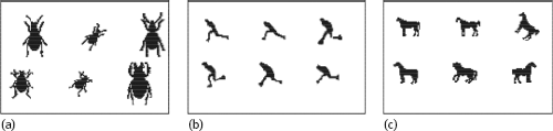
Some of the above properties of this descriptor are illustrated in Figure 7.1 (ISO/IEC, 2001), and each frame contains very similar images according to CSS, based on the actual retrieval results from the MPEG-7 shape database. Figure 7.1(a) shows shape generalization properties (perceptual similarity among different shapes). Figure 7.1(b) shows the robustness to nonrigid motion (man running). Figure 7.1(c) shows the robustness to partial occlusions (tails or legs of the horses).

Example 7.1 Various shapes described by shape descriptors

The shape of an object may consist of a single region or a set of regions as well as some holes in the object as illustrated in Figure 7.2. Note that the black pixel within the object corresponds to 1 in an image, while the white background corresponds to 0. Since the region shape descriptor makes use of all pixels constituting the shape within a frame, it can describe any shape. In other words, the region shape descriptor can describe not only a simple shape with a single connected region as in Figure 7.2(a, b) but also a complex shape that consists of holes in the object or several disjoint regions as illustrated in Figure 7.2(c–e), respectively. The region shape descriptor not only can describe such diverse shapes efficiently in a single descriptor but also is robust to minor deformations along the boundary of the object.

Figure 7.2(g–i) are very similar shape images for a cup. The differences are at the handle. Shape in (g) has a crack at the lower handle, while the handle in (i) is filled. The region-based shape descriptor considers Figure 7.2 (g, h) to be similar but different from Figure 7.2(i) because the handle is filled. Similarly, Figure 7.2(j, k), and 7.2(l) show the part of video sequence where two disks are being separated. With the region-based descriptor, they are considered similar.

The descriptor is also characterized by its small size, fast extraction time, and matching. The data size for this representation is fixed to 17.5 bytes. The feature extraction and matching processes are straightforward and have a low order of computational complexities, and suitable for tracking shapes in the video data processing.

7.1.3.2Shape Descriptor Based on Wavelet Modulus Maxima and Invariant Moments

Since the wavelet coefficients are obtained by sampling uniformly the continuous wavelet transform via a dyadic scheme, the general discrete wavelet transform lacks the translation invariance. A solution is to use the adaptive sampling scheme. This can be achieved via the wavelet modulus maxima, which are based on irregular sampling of the multiscale wavelet transform at points that have some physical significance. Unlike regular sampling, such a sampling strategy makes the translation invariance of the representation (Cvetkovic, 1995). In two dimensions, the wavelet modulus maxima indicate the location of edges (Mallat, 1992).

Example 7.2 Illustration of wavelet modulus maxima

In the first row of Figure 7.3, an original image is given. The second row shows seven images of the wavelet modulus in seven scales (the scale increases from left to right). The third row shows the corresponding maxima of wavelet modulus. Visually, the wavelet modulus maxima of an image are located along the edges of the image (Yao, 1999).

It has been proven that for an N × N image, the levels of the wavelet decomposition J should not be higher than J = log2(N) + 1. Experimental results show that the wavelet maxima at a level higher than 6 have almost no discrimination power. For different applications, different levels of wavelet decomposition can be selected. Fewer decomposition levels (about 1 to 2 levels) can be used in retrieving a clothes-image database to save computation, and more decomposition levels (5 to 6 levels) can be used in retrieving a flower-image database to extract enough shape information of the image.

Given a wavelet representation of images, the next step is to define a good similarity measurement. Considering the invariance with respect to affine transforms, the invariant moments can be selected as the similarity measurement.

The moments extracted from the image form a feature vector. The feature elements in the vector are different physical quantities. Their magnitudes can vary drastically, thereby biasing the Euclidean distance measurement. Therefore, a feature normalization process is thus needed. Let F = [f1, f2,..., fi,..., fN] be the feature vector, where N is the number of feature elements and let I1, I2, ..., IM be the images. For image Ii, the corresponding feature F is referred to as Fi = [f1,i, f2,...,fij,...,fN]. Since there are M images in the database, an M × N feature matrix F = {fi,j} can be formed, where fi,j is the j-th feature element in Fi. Now, each column of F is a sequence with a length M of the j-th feature element, represented as Fi. Assuming Fi to be a Gaussian sequence, the mean mj and the standard deviation σj of the sequence are computed. Then, the original sequence is normalized to an N(0,1) sequence as follows

$f_{i,j}=\frac{f_{i,j}-m_j}{{\sigma }_j}\left(7.15\right)$

The main steps of this algorithm can be summarized as follows (further details can be found in Zhang (2003b):

(1)Make the wavelet decomposition of the image to get the module image.

(2)Compute the wavelet modulus maxima to produce the multi-scale edge image.

(3)Compute the invariant moments of the multiscale edge image.

(4)Form the feature vector based on the moments.

(5)Normalize (internally) the magnitudes among different feature elements in the feature vector.

(6)Compute the image similarity by using their feature vectors.

(7)Retrieve the corresponding images.

Example 7.3 Retrieval results for geometrical images

Figure 7.4 gives two sets of results in retrieving geometric figures. In the presentation of these results, the query image is at the top-left corner and retrieving images are ranked from left to right, top to bottom. Under the result images, the similarity values are displayed. As shown in Figure 7.4, the above algorithm ranks the image of the same shape images (regardless of its translation, scaling, and rotation) as better matches. It is evident that this algorithm is invariant to translation, scaling, and rotation.

7.2Motion-Feature-Based Video Retrieval

Motion information represents the evolution of video content along the time axis, which is important for understanding the video content. It is worth noting that color, texture, and shape are common features for both images and video, while motion feature is unique for video.

Motion information in video can be divided into two categories: global motion information and local motion information.

7.2.1Global Motion Features

Global motion corresponds to the background motion, which is caused by the movement of cameras (also called camera motion) and characterized by the integer movement of all points in a frame. Global motion for a whole frame can be modeled by a 2-D motion vector (Tekalp, 1995).

Motion analysis can be classified into short-time analysis (for a few frames) and long-time analysis (several 100 frames). For a video sequence, short-time analysis can provide accurate estimation about the motion information. However, for understanding a movement, a duration of about one second or more is required. To obtain the meaningful motion content, a sequence of short-time analysis results should be used. Each of the short-time analysis results can be considered a point in the motion feature space, so the motion in an interval can be represented as a sequence of feature points (Yu, 2001b). This sequence includes not only the motion information in adjacent frames but also the time ordering relation in video sequence.

The similarity measurement for feature-point sequences can be carried out with the help of string matching (another possibility is to use subgraph isomorphism introduced in Section 4.5), as introduced in Section 4.2. Suppose that there are two video clips l1 and l2, whose lengths of the feature point sequences are N1 and N2, then these two feature point sequences can be represented by {f1(i) i = 1, 2, ···, N1} and {f(j), j = 1,2, ·· ·, N2}, respectively. If the lengths of two sequences are the same, that is, N1 = N2 = N, the similarity between two sequences is

$S\left(l_1,l_2\right)={\displaystyle \sum _{i-1}^N{S}_f\left[f_1\left(i\right),f_2\left(i\right)\right]}\left(7.16\right)$

where Sf[f1(i), f2(i)] is a function for computing the similarity between two feature points, which can be the reciprocal of any distance function.

If two sequences have different lengths, N1 < N2, then the problem of selecting the beginning point for matching should be solved. In practice, different sequences $l_2^{\text{'}}\left(t\right)$ with the length equal to that of l1 in l2 with a different beginning time t are selected. Since $l_2^{\text{'}}\left(t\right)$ have the same lengths, the distance between them can be computed with eq. (7.16). By changing the beginning time, the similarity values for all possible subsequences can be obtained, and the similarity between l1 and l2 is determined as the maximum of these values

$S\left(l_1,l_2\right)=\underset{0\le t\le N_2-N_1}{{\displaystyle \max }}{\displaystyle \sum _{i-1}^N{S}_f\left[f_1\left(i\right),f_2\left(i+t\right)\right]}.\left(7.17\right)$

7.2.2Local Motion Features

Local motion corresponds to the foreground motion, which is caused by the movement of the objects in the scene. Since many objects can exist in one scene and different objects can move differently (in directions, speed, form, etc.), local motion can be quite complicated. For one image, the local motions inside may need to be represented with several models (Yu, 2001a).

To extract local motion information from a video sequence, the spatial positions of the object’s points in different frames of the video should be searched and determined. In addition, those points corresponding to the same object or the same part of the object, which have the same or similar motions, should be connected, to provide the motion representations and descriptions of the object or part of the object.

The motion representations and descriptions of objects often use the vector field of local motion, which provides the magnitude and direction of motion. It is shown that the direction of motion is very important in differentiating different motions. A directional histogram of local motion can be used to describe local motion. On the other hand, based on the obtained vector field of the local motion, the frame can be segmented and those motion regions with different model parameters can be extracted. By classifying the motion models, a histogram for the local motion region can be obtained. Since the parameter models of motion regions are the summarization of the local motion information, the histogram of the local motion region often has a higher level meaning and a more comprehensive description ability. The matching for these histograms can also be carried out by using the methods such as histogram intersection, as shown in Section 7.1.

Example 7.4 Feature matching with two types of histograms

Illustrations for using the above two histograms are shown below by an experiment. In this experiment, a video sequence of nine minutes for a basketball match, which comes from an MPEG-7 standard test database, is used. Figure 7.5 shows the first frame of a penalty shot clip, which is used for querying.

In this video sequence, except for the clip whose first frame is shown in Figure 7.5, there are five clips with similar content (penalty shot). Figure 7.6 shows the first frames of four clips retrieved by using the directional histogram of the local motion vector. From Figure 7.6, it can be seen that although the sizes and positions of regions occupied by players are different, the actions performed by these players are all penalty shots. Note that the player in Figure 7.6(a) is the same as that in Figure 7.5, but these two clips correspond to two scenes.

Figure 7.7 shows the first frames of another clip retrieved using the histogram of the local motion vector. In fact, all five clips with penalty shots have been retrieved by this method. Compared to the directional histogram of the local motion vector, the histogram of the local motion vector provides better retrieval results.

In the above discussion, the global and local motions are considered separately, and also detected separately. In real applications, both the global motion and the local motion will be included in video. In this case, it is required to first detect the global motion (corresponding to the motion in the background where there is no moving object), and then to compensate the global motion to remove the influence of the camera motion, and finally to obtain the local motion information corresponding to different foreground objects. As many global motion and local motion information can be obtained directly from a compressed domain, the motion-feature-based retrieval can also be performed directly in a compressed domain (Zhang, 2003b).

7.3Object-Based Retrieval

How to describe an image’s contents is a key issue in content-based image retrieval. In other words, among the techniques for image retrieval, the image content description model would be a crucial one. Humans’ understanding of image contents possesses several fuzzy characteristics, which indicates that the traditional image description model based on low-level image features (such as color, texture, shape, etc.) is not always consistent to human visual perception. Some high-level semantic description models are needed.

7.3.1Multilayer Description Model

The gap between low-level image features and high-level image semantics, called the semantic gap, sometimes leads to disappointing querying results. To improve the performance of image retrieval, there is a strong tendency in the field of image retrieval to analyze images in a hierarchical way and to describe image contents on a semantic level. A widely accepted method for obtaining semantics is to process the whole image on different levels, which reflects the fuzzy characteristics of the image contents.

In the following, a multilayer description model (MDM) for image description is depicted (see Figure 7.8); this model can describe the image content with a hierarchical structure to reach progressive image analysis and understanding (Gao, 2000b). The whole procedure has been represented in four layers: The original image layer, the meaningful region layer, the visual perception layer, and the object layer. The description for a higher layer could be generated from the description from the adjacent lower layer, and the image model is synchronously established by the procedure for progressive understanding of the image contents. These different layers could provide distinct information on the image content; so this model is suitable for accessing from different levels.

In Figure 7.8, the left part shows that the proposed image model includes four layers, in which the middle part shows the corresponding formulas for the representations of the four layers, while the right part provides some representation examples of the four layers.

In this model, the image content is analyzed and represented in four layers. The adjacent layers are structured in a way that the representations for the upper layers are directly extracted from those for lower layers. The first step is to split the original image into several meaningful regions, each of which provides certain semantics in terms of human beings’ understanding of the image contents. Then proper features should be extracted from these meaningful regions to represent the image content at the visual perception layer. In the interest of the follow-up processing, such as object recognition, the image features should be selected carefully. The automatic object recognition overcomes the disadvantage of large overhead in manual labeling while throws off the drawback of insufficient content information representation by using only lower-level image features. Another important part of the object layer process is relationship determination, which provides more semantic information among the different objects of an image.

Based on the above statements, the multilayer description model could be expressed by the following formula

$\mathit{\text{MDM=}}\left\{\mathit{\text{OIL,MRL,VPL,OL}}\right\}\left(7.18\right)$

In eq. (7.18), OIL represents the lowest layer − the original image layer − with the original image data represented by f(x, y). MRL represents the labeled image l(x, y), which is the result of the meaningful region extraction (Luo, 2001). VPL is the description for the visual perception layer, and it contains three elements, FMC, FWT and FRD, representing mixed color features, wavelet package texture features, and region descriptors, respectively (Gao, 2000a). The selection of VPL is flexible and it should be based on the implementation. OL is the representation of the object layer and it includes two components, T and Rs. The former T is the result of the object recognition used to indicate the attribute of each extracted meaningful region, for which detailed discussions would be given later. The latter Rs is a K × K matrix to indicate the spatial relationship between every two meaningful regions, with K representing the number of the meaningful regions in the whole image.

In brief, all the four layers together form a “bottom-up” procedure (implying a hierarchical image process) of the multilayer image content analysis. This procedure aims at analyzing the image in different levels so that the image content representation can be obtained from low levels to high levels gradually.

7.3.2Experiments on Object-Based Retrieval

Some experiments using the above model for a multilayer description for the object-based retrieval are presented below as examples. In these experiments, landscape images are chosen as the data source. Seven object categories often found in landscape images are selected, which include mountain, tree, ground, water, sky, building, and flower.

7.3.2.1Object Recognition

In Figure 7.9, four examples of the object recognition are presented. The first row is for original images. The second row gives the extracted meaningful regions. As is mentioned above, the procedure of meaningful region extraction aims not at precise segmenting but rather at extracting major regions, which are striking to human vision. The third row represents the result of the object recognition, with each meaningful region labeled by different shades (see the fourth row) to indicate the belonging category.

7.3.2.2Image Retrieval Based on Object Matching

Based on object recognition, the retrieval can be conducted in the object level. One example is shown in Figure 7.10. The user has submitted a query in which three objects, “mountain,” “tree,” and “sky,” are selected to query. Based on this information, the system searches in the database and looks for images with these three objects. The returned images from the image database are displayed in Figure 7.10. Though these images are different in the sense of the visual perception as they may have different colors, shapes, or structural appearances, all these images contain the required three objects.

Based on object recognition, the retrieval can be further conducted using the object relationship. One example is given in Figure 7.11, which is a result of an advanced search. Suppose the user made a further requirement based on the querying results of Figure 7.10, in which the spatial relationship between the objects “mountain” and “tree” should also satisfy a “left-to-right” relationship. In other words, not only the objects “mountain” and “tree” should be presented in the returned images (the presentation of “sky” objects is implicit), but also the “mountain” should be presented to the left of the “tree” in the images (in this example, the position of “sky” is not limited). The results shown in Figure 7.11 are just a subset of Figure 7.10.

7.4Video Analysis and Retrieval

The purpose of video analysis is to establish/recover the semantic structure of video (Zhang, 2002b). Based on this structure, further querying and retrieval can be easily carried out. Many video programs exist, such as advertisements, animations, entertainments, films, home videos, news, sport matches, teleplays, etc.

7.4.1News Program Structuring

A common video clip is physically made up of frames, and the video structuring begins with identifying each individual camera shots of the frames. Video shots serve as elementary units used to index the complete video clips. Many techniques for shot boundary detection have been proposed (O’Toole, 1999; Garqi, 2000; and Gao, 2002a).

7.4.1.1Characteristics of News Program

A news program has a consistent, regular structure that is composed of a sequence of news story units. A news story unit is often called a news item, which is naturally a semantic content unit and contains several shots, each of which presents an event with a relative independency and clear semantics. In this way, the news story unit is the basic unit for video analysis.

The relatively fixed structure of news programs provides many cues for understanding the video content, establishing index structure, and performing content-based querying. These cues can exist on different structure layers and provide relatively independent video stamps. For example, there are many speakers’ shot in which the speakers or announcers repeatedly appear. This shot can be considered the beginning mark of a news item and is often called an anchor shot. Anchor shots can be used as hypothesized beginning points for news items.

In news program analysis, the detection of anchor shots is the basis of video structuring. Two types of methods are used in the detection of anchor shots: The direct detection and the rejection of no-anchor shot. One problem for correctly detecting an anchor shot is that there are many “speakers’ shot” in news programs, such as reporter shots, staff shots, and lecturer shots, etc. All these shots are mixed, so the accurate detection of anchor shots is difficult, and many false alarms and wrong detections could happen.

In the following, a three-step detection method for anchor shots is presented (Jiang, 2005a). The first step is to detect all main speaker close-ups (MSC) according to the changes among consecutive frames. The results include real anchor shots but also some wrong detections. The second step is to cluster MSC using unsupervised clustering method and to establish a list of MSC (some postprocesses are made following the results of news title detection). The third step is to analyze the time distribution of shots and to distinguish anchor shots from other MSC shots.

7.4.1.2Detection of MSC

The anchor shot detection is frequently relied on the detection of anchorpersons, which is often interfered by other persons, such as reporters, interviewees, and lecturers. One way to solve this problem is by adding a few preprocessing (Albjol, 2002) or postprocessing (Avrithis, 2000) steps to prevent the possible false alarms. However, in the view of employing rather than rejecting the interferences, one can take proper steps to extract visual information from these “false alarms” and use the special information that gives clues to the video content structuring and facilitate the anchor shot identification.

Since a dominant portion of news programs is about human activities, human images, and especially those camera-focused talking heads play an important role. With an observation of common news clips, it is easily noticed that heads of presidents or ministers appear in political news, heads of pop stars or athletes appear in amusement or sports news, and heads of professors or instructors appear in scientific news, etc. Definitely, these persons are the ones users are looking for when browsing news video. Therefore, apart from being a good hint for the existence of anchorpersons, all the focused heads themselves serve as a good abstraction of news content regarding to key persons.

The detection of a human subject is particularly important here to find MSC shots. As it is defined, MSC denotes a special scene with a single focused talking head in the center of each frame, whose identification is possible using a number of human face detection algorithms. However, it is not concerned here with the face details such as whether it has clear outlines of cheeks, nose, or chin. What gives the most important clues at this point is whether it is a focused talking head in front of the camera with the probability of belonging to anchorpersons, or some meaningless objects and the backgrounds. In terms of this viewpoint, skin color and face shape are not the necessary features that must be extracted. Thus, differing from other methods based on complicated face color/shape model training and matching (Hanjalic, 1998), identifying MSCs in a video stream can be carried out by motion analysis in a shot, with a simplified Head-Motion-Model set. Some spatial and motional features of the MSC frame are illustrated in Figure 7.12.

(1)Generally, an MSC shot (see Figure 7.12(b)) has relatively lower activity compared to normal shots (see Figure 7.12(c)) in news video streams, but has stronger activity than static scene shots (see Figure 7.12(a)).

(2)Each MSC has a static camera perspective, and activity concentrates on a single dominant talking head in the center of the frame, with a size and position within a specific range.

(3)In MSC shots, the presence of a talking head is located in a fixed horizontal area during the shot, with three typical positions: left (L), middle (M), and right (R), as shown in Figure 7.12(d–f).

According to the above features, MSC detection can be carried out with the help of the map of average motion in shot (MAMS) (Jiang, 2005a). For the k-th shot, its MAMS is computed by

$M_k\left(x,y\right)=\frac{1}{L}{\displaystyle \sum _{i-1}^{L-d}\left|f_i\left(x,y\right)-f_{i+d}\left(x,y\right)\right|}L=\frac{N}{d}\left(7.19\right)$

where N is the number of frames in the k-th shot and d is the interval between the measured frames.

MAMS is a 2-D cumulative motion map, which keeps the spatial distribution of the motion information. The change value of an MSC shot is between that of the normal shots and that of static scene shots, and can be described by the division of MAMS by its size. In other words, only the following shot can be a possible candidate

$T_s<\frac{M_k\left(x,y\right)}{N_x\times N_y}<T_n\left(7.20\right)$

where Ts and Tn are the average values of static scene shots and normal shots, respectively.

7.4.1.3Clustering of MSC shots

The extracted MSCs serve as a good abstraction of news content in phase of key persons. Actually, it is not effective to browse all MSCs one by one, to search somebody in particular. Some MSC navigation and indexing schemes are needed. Since the same “main speaker” usually has similar appearances (like clothes’ color and body size) in various shots during one news program, human clustering is used to build up an index table. With the guide of this table, the retrieval of key persons can be supported in an immediate way.

The MSC clustering algorithm uses color histogram intersection (CHI) as the similarity metrics. Since the acquired head positions (L/M/R), as shown in Figure 7.12(d–f), suggest three corresponding body areas, which can be also called left/middle/right body positions, three position models can be established for an unsupervised clustering. After clustering, the separation of anchor groups from other groups can be conducted when considering the duration, proportion, distribution, and frequency of typical anchor shots. The thresholds used are chosen empirically. A large amount of video data (more than 6 hours of news programs from the MPEG-7 Video Content Set) with four possible distinct features, shot length, total number of shots, shot interval, and time range of all shots, are investigated. Some averaged statistics are collected in Table 7.1.

From Table 7.1, it can be seen that the shot number, the shot interval, and the time range have good discriminate power. Compared to other groups, the anchor group is repeated more frequently. The following criteria can be used to separate or extract anchor shots from other MSC shots:

(1)The total number of shots of this type is greater than a threshold.

(2)The average interval between two adjacent shots of this type is greater than a threshold.

(3)The distance between the first and last shots (time range) of this type is greater than a threshold.

Using the above criteria, MSC shots can be classified into two types: One is anchor shots (represented by A1, A2, ...) and the other is other person shots (represented by P1, P2, ...). For each news item, taking the appearance of an anchor shot as the beginning position, followed by related report shots and speaker’s shots, a structured news program is obtained. One example is shown in Figure 7.13. Using this structure, a user could locate any specific person in any news item and perform non-linear high-level browsing and querying (Zhang, 2003b).