5Scene Analysis and Semantic Interpretation

Image understanding actually is to achieve understanding of the scene. Understanding of the visual scene can be expressed as follows: on the basis of visual perception of environmental data, combined with a variety of image technology, from the perspective of statistics of calculation, cognitive of behavior, semantic interpretation, and so on, mining the characteristics and patterns of visual data, to achieve the effective explanation and cognition of scene. From a certain point of view, the scene understanding is based on the scene analysis, to achieve the goal of interpreting the scene semantics.

Scene understanding requires the incorporation of high-level semantics. The scene labeling and classification are both the means of scene analysis toward the semantic interpretation of scene. On the other side, to explain the semantics of the scene, it is required to make further reasoning according to the processing and analysis results of the image data. Reasoning is the process of collecting information, performing learning, making decisions based on logic. There are many other mathematical theories and methods can be used in scene understanding.

The sections of this chapter are arranged as follows:

Section 5.1 provides a summary of the various scenarios and different tasks involved in scene understanding.

Section 5.2 discusses fuzzy reasoning. Based on the introduction to the concepts of fuzzy sets and fuzzy operations, the basic fuzzy inference methods are outlined.

Section 5.3 describes a method of using genetic algorithms for image segmentation and semantic decomposition, as well as semantic inference judgment.

Section 5.4 focuses on the question of scene object labeling. Labeling to scene objects is an important means to enhance the results of the analysis into the conceptual level, commonly used methods include discrete labeling and probability labeling.

Section 5.5 discusses around the scene classification and introduces some of the definitions, concepts, and methods, primarily the bag of words model/the bag of features model, pLSA model, and LDA model.

5.1Overview of Scene Understanding

Scene analysis and semantic interpretation are important to understand the content of the scene, but the research is relatively less mature in this area, many of the issues are still in exploration and evolution.

5.1.1Scene Analysis

Scene analysis must rely on image analysis techniques to obtain information on the subjects in the scene. Scene analysis is thus to build the foundation for further scene interpretation.

Object recognition is an important step and one of the foundations for scene analysis. When recognizing a single object, it is generally believed that the image of this object region can be decomposed into several subregions (often corresponding to the part of object), these subregions have relatively fixed geometry, and they together constitute the appearance of the object. But in the analysis of natural scenes, which often contains a number of scene subjects, the relationship among them is very complex and quite difficult to predict, so in the scene analysis not only the internal relationship among objects themselves but also the distribution and relative position of different objects should be considered.

From a cognitive perspective, scene analysis is more concerned about people’s perception and understanding of the scene. A large number of biology, physiology, and psychology tests for scene analysis showed that the global characteristic analysis of the scene often occurs in the early stage of visual attention. How to lay on the research results of biology, physiology, and psychology, and introducing the corresponding constraint mechanism to establish a reasonable calculation model are the issues requiring research and exploration.

In the scene analysis, an important issue is that the visual content of the scene (the objects and their distribution) would have large uncertainty due to:

(1)Different lighting conditions, which can lead to difficulties on object detection and tracking

(2)Different object appearances (although sometimes they have similar structural elements), which will bring ambiguity to the identification of objects in scene

(3)Different observation scales, which often affect the identification and classification of the objects in scene

(4)Different landscape positions, orientations and occlusions among each other, which will increase the complexity of object cognition

5.1.2Scene Perception Layer

Analysis and semantic interpretation of the scene can be conducted at different levels. Similar in content-based coding, the model-based coding can be performed at three levels, namely the lowest level of object-based coding; the middle level of knowledge-based coding; and the highest level of semantic-based coding. The analysis and semantic interpretation of the scene can be divided into three layers.

(1)Local layer: The main emphasis on this layer is the analysis, recognition or labeling of image region for local scene or single object.

(2)Global layer: This layer considers the whole scene, focuses on the relationship between objects having a similar appearance and functionality, and so on.

(3)Abstraction layer: This layer corresponds to the concept meaning of the scene and provides the abstract description of scene.

Taking the scene of the course conduction in a classroom as an example, the three layers corresponding to the above analysis and semantic interpretation task can be considered as follows. In the first layer, the main consideration is on extracting objects from the image, such as teachers, students, tables, chairs, screens, projectors, and so on. At the second layer, the focus is on determining the position and the mutual relationship of the objects, such as the teacher standing in front of the classroom, students sitting facing the screen, the projector projecting the lecture notes toward screen, and so on; the focus is also on analyzing environment and functionality, such as indoor or outdoor, what type of indoor rooms (office or classroom), and so on. At the third layer 3, it is required to describe the activities in the classroom (such as inclass or recess) and/or the atmosphere (such as serious or more relaxed, calmer or very dynamic).

Humans have a strong capability for the perception of scene. For a new scene (especially the more conceptual scene), the human eye has often swept once to explain the meaning of the scene. For example, considering an open sport game in the playground, by observing the color of the grass and runway (low-level features), the athletes and running state (intermediate target) on the runway, plus the reasoning based on experience and knowledge (conceptual level), people could immediately make the correct judgment. In this process, the perception of middle layer has a certain priority. Some studies have shown that people have a strong ability to identify middle-layer objects (such as stadium), which is faster than identifying and naming them at lower and/or upper layers. There are some hypotheses that the higher priority of perception in the middle layer comes from two factors within the same time: one is maximizing the similarity inside classes (if there is or no athlete in playground), another is maximizing the difference between classes (even the classrooms after class will be different from the playground). From the visual characteristics of the scene itself, the same objects in the middle layer have often a similar spatial structure, and perform similar behaviors.

In order to obtain the semantic interpretation of the scene, it is required to establish connection between the high-level concepts with the low-level visual features and middle-level object properties, as well as to recognize objects and their relative relationship. To accomplish this work, two modeling methods can be considered.

5.1.2.1Lower Scenario Modeling

Such methods directly represent and describe the low-level properties (color, texture, etc.) of the scene, and then reasoning based on the high-level information for a scene by means of classification and recognition. For example, there is a large playground with grass (light green), track (dark red); there are classrooms with many desks and chairs (regular geometry having horizontal or vertical edges).

The methods can be further divided into:

(1)Global method: it works with the help of statistics of the whole image (such as color histograms) to describe the scene. A typical example is the classification of images into indoor images and outdoor images, the outdoor images can be further divided into natural outdoor scenery images and artificial building images, the artificial building images can be still further divided into tower images, playground images, and so on.

(2)Block method: It works on dividing the image into multiple image pieces called blocks (can be regular or irregular). For each block, the global method can be used, and then these results can be integrated to provide the judgment.

5.1.2.2Middle Semantic Modeling

Such methods improve the performance of low-level feature classification by means of identification of objects, and solve the semantic gap problem between high-level concepts and low-level attributes. A commonly used method is based on classifying the scene into specific semantic categories according to the semantics and distribution of objects, by using visual vocabulary modeling (see Section 5.5.1). For example, the determination of the classroom from the indoor scene can be performed with the existence of objects such as tables, chairs, projector/projection screen and so on. Note that the semantic meanings of the scene may not be unique, and indeed it is often not unique in practice (e. g., the projector can be in a classroom or in a conference room). Especially for outdoor scenes, the situation would be more complicated, because the objects in scene can have any size, shape, location, orientation, lighting, shadows, occlusion, and so on. In addition, several individuals of the same type of objects may also have quite different appearances.

5.1.3Scene Semantic Interpretation

Scene semantic interpretation is a multi-faceted research and development of technology:

(1)Visual computing technology;

(2)Dynamic control strategy of vision algorithms;

(3)Self-learning of scene information;

(4)Rapid or real-time computing technology;

(5)Cooperative multi-sensory fusion;

(6)Visual attention mechanism

(7)Scene interpretation combining cognitive theory;

(8)System integration and optimization.

5.2Fuzzy Reasoning

Fuzzy is a concept often associated with the opposites of clear or precise (crisp). In daily life, many obscure things may be encountered, which have no clear amount or quantitative limits, then some vague phrases should be used for description. Fuzzy concepts can express a wide variety of noncritical, uncertain, imprecise knowledge and information, as well as those obtained from conflicting sources. Here it is possible to use human-like qualifiers or modifiers, such as higher intensity, lower gray value, and so on, to form fuzzy sets and to express the knowledge about image. Based on the expression of knowledge, further reasoning can be conducted. Fuzzy inference needs the help of fuzzy logic, fuzzy operation, and fuzzy arithmetic/algebra.

5.2.1Fuzzy Sets and Fuzzy Operation

A fuzzy set S in a fuzzy space X is a set of ordered pairs:

$S=\left\{\left[x,M_S\left(x\right)\right]|x\in X\right\}\left(5.1\right)$

where MS(x) represents the grade of membership of x in S. The values of membership function are always nonnegative real numbers and are normally limited in [0, 1]. The fuzzy sets are described solely by its membership function. Figure 5.1 shows some examples of using crisp set and fuzzy set to represent the concept “dark,” where the horizontal axis corresponds to image gray-level x that would be the domain of definition of membership function for fuzzy set, and the vertical axis shows the values of membership function L(x). Figure 5.1(a) uses crisp sets to describe “dark,” and the result is binary (gray level smaller than 127 is complete dark, while gray level bigger than 127 is entirely no dark). Figure 5.1(b) is a typical fuzzy membership function that has value from 1 to 0, corresponds to gray-level values from 0 to 255. When x is 0, the L(x) is 1, x is completely belong to dark fuzzy set. When x is 1, the L(x)is 0, x does not completely belong to dark fuzzy sets. Between these two extremes, the gradual transition of x indicates that some intermediate parts belong to “dark,” while other parts are not under the “dark.” Figure 5.1(c) is a nonlinear membership function. It looks like a combination of Figure 5.1(a, b), but it still represents a fuzzy set.

Operations on fuzzy sets can be carried out by using fuzzy logic operations. Fuzzy logic is built on the basis of multi-valued logic. It studies the means of fuzzy thinking, language forms and laws with fuzzy sets. In fuzzy logic operations, there are some operations having similar names with that in general logic operations but with different definitions. Let LA(x) and LB(y) represent membership functions corresponding to fuzzy sets A and B, their domains of definitions are X and Y, respectively. The fuzzy intersection, fuzzy union, and fuzzy complement can be defined as follows

$\begin{array}{c}\text{Intersection}A\cap B:L_{A\cap B}\left(x,y\right)=\min \left[L_A\left(x\right),L_B\left(y\right)\right]\\ \text{Union}A\cup B:L_{A\cup B}\left(x,y\right)=\max \left[L_A\left(x\right),L_B\left(y\right)\right]\left(5.2\right)\\ \text{Complement}{A}^c:L_{A^c}\left(x\right)=1-L_A\left(x\right)\end{array}$

Operations on fuzzy sets can also be achieved by using the normal algebra operations via point by point changing the shape of the fuzzy membership function. Suppose the membership function in Figure 5.1(a) represents a fuzzy set D (dark), then the membership function of an enhanced fuzzy set VD (very dark) would be (as shown in Figure 5.2(a)):

$L_{\text{VD}}\left(x\right)=L_D\left(x\right).L_D\left(x\right)=L_D^2\left(x\right)\left(5.3\right)$

This kind of operations can be repeated. For example, the membership function of fuzzy set VVD (very very dark) would be (as shown in Figure 5.2(b)):

$L_{\text{VVD}}\left(x\right)=L_D^2\left(x\right).L_D^2\left(x\right)=L_D^4\left(x\right)\left(5.4\right)$

On the other side, it is possible to define a weak fuzzy set SD (somewhat dark), whose membership function is (as shown in Figure 5.2(c)):

$L_{\text{SD}}\left(x\right)=\sqrt{L_{\text{D}}\left(x\right)}\left(5.5\right)$

Logical operations and algebra operations can also be combined. For example, the membership function of fuzzy set NVD (not very dark), that is, the complement of enhanced fuzzy set VD, is (as shown in Figure 5.2(d)):

$L_{\text{NVD}}\left(x\right)=1-L_{\text{D}}^2\left(x\right)\left(5.6\right)$

Here NVD can be seen as N[V(D)], so LD(x) corresponds to $D,L_D^2\left(x\right)$ corresponds to V(D) and $1-L_D^2\left(x\right)$ corresponds to N[V(D)].

5.2.2Fuzzy Reasoning Methods

In fuzzy reasoning, the information in several fuzzy sets is combined according to certain rules to make a decision, Sonka (2008).

5.2.2.1BasicModel

The basic model and main steps for fuzzy reasoning are shown in Figure 5.3. Starting from fuzzy rules, the determination of the basic relations of the memberships in associated membership functions is called composition. The result of fuzzy composition is a fuzzy solution space. Making a decision on the basis of solution space, a de-fuzzification (de-composition) process is required.

Fuzzy rules are a series of unconditional and conditional propositions. The form of unconditional fuzzy rules is

$x\text{is}A\left(5.7\right)$

The form of conditional fuzzy rules is

$\text{if}x\text{is}A\text{then}yisB\left(5.8\right)$

where A and B are fuzzy sets, x and y represent scales from their respective domains.

The membership that corresponds to unconditional fuzzy rules is LA(x). The unconditional fuzzy propositions are used to limit solution space or to define a default solution space. Since these rules are unconditional, they can be used directly to solution space with the help of fuzzy set operations.

It is now considering the conditional fuzzy rules. Among the currently used methods for decision, the simplest is the monotonic fuzzy reasoning. It can directly obtain the solution without the use of fuzzy composition and de-fuzzification (see below). For example, let x represent the outside illumination value, y represent gray-level value of image, then the fuzzy rule representing the high-low gray level of image is: if x is DARK then y is LOW.

The principle of monotonic fuzzy reasoning is shown in Figure 5.4. Suppose the outside illumination value is x = 0.3, then the membership value is LD(0.3) = 0.4. If this value is used to represent membership value LL(y)LD(x), then the expectation of high-low gray level of image is y = 110, which is at a relative low place in the range from 0 to 255.

5.2.2.2Fuzzy Composition

The knowledge related to decision-making processes is often included in more than one fuzzy rule. However, it is not every fuzzy rule for decision making that has the same contribution. There are different rules for combining the binding mechanism, the most commonly used approach is the min-max rule.

In the min-max composition, a series of minimization and maximization processes are used. One example is shown in Figure 5.5. First, the correlation minimum (the minimum of the predicate truth) LAi(x) is used to restrict the consequent fuzzy membership function LBi(y), where i represents the ith rule (two rules are used in this example). Then, the consequent fuzzy membership function LBi(y) is updated point by point to produce the fuzzy membership function:

$L_{B_l^{+}}\left(y\right)=\min \left\{L_{Al}\left(x\right),L_{Bl}\left(y\right)\right\}\left(5.9\right)$

Finally, by seeking the maximum of minimized fuzzy set, point by point, the fuzzy membership function of solutions is

$L_S\left(y\right)=\underset{l}{\max }\left\{L_{B_l^{+}}\left(y\right)\right\}\left(5.10\right)$

Another approach is called correlation product. One example is given in Figure 5.6. This approach scales the original consequent membership function instead of truncating them. Correlation minimum has the advantage of being computationally simple and easier to de-fuzzify. Correlation product has the advantage of keeping the original form of fuzzy set, as shown in Figure 5.6.

5.2.2.3De-fuzzification

Fuzzy composition gives the fuzzy membership function of one single solution for each solution variable. To determine the exact solutions used for decision making, it is required to identify a vector that can best express the information in fuzzy solution set and has multiple scalars (each corresponding to a solution variable). This process should be carried out independently for each solution variable, and is called de-fuzzification. Two commonly used de-fuzzification methods are the moment composition method and the maximum composition method.

The moment composition method first determines the centroid of membership function of fuzzy solution c, and then converts the fuzzy solution into a crisp solution variable c, as shown in Figure 5.7(a). The maximum composition method determines the domain point where the membership function has maximum value among the membership functions of fuzzy solution. In case the maximum values are at a plateau, then the center of the plateau provides a crisp solution d, as shown in Figure 5.7(b). The moment composition method is result sensitive to all rules, while the maximum composition method has results depending on the single rule with maximum predicate value. The moment composition method is often used for control applications, while the maximum composition method is often used in recognition applications.

5.3Image Interpretation with Genetic Algorithms

A brief description for the basic ideas and operations of genetic algorithms is given, and using genetic algorithms for image segmentation and semantic content explanation is provided.

5.3.1Principle of Genetic Algorithms

Genetic algorithms (GA) use the natural evolution mechanism to search the extremes of objective function. Genetic algorithms are not guaranteed to find the global optimum, but in practice it can always find solutions very closing to the global optimal solution. Genetic algorithms have some properties compared to other optimization techniques:

(1)Genetic algorithms do not use parameter sets themselves but use a coding of these sets. Genetic algorithms require the natural parameter sets to be coded as a finite-length string with limited symbols. In this way, the representation for every optimization problem is converted to a string representation. In practice, binary strings are often used, in which there are only two symbols, 0 and 1.

(2)In each extreme search step, genetic algorithms look from a large population of sample points, instead of a single point. Thus, it has a great chance to find the global optimum.

(3)Genetic algorithms directly use the objective function, instead of using derivatives or auxiliary knowledge. The search for new and better solutions depends only on the evaluation function that can describe the goodness of the particular string. The value of the evaluation function in genetic algorithms is called fitness.

(4)Genetic algorithms do not use the deterministic rules, but use probabilistic transition rules. The transition rules from the current string populations to new and better string populations depends only on the natural idea, that is, according to higher fitness to support good string while removing bad string with only lower fitness. This is just the basic principle of genetic algorithms, in which the string with the best result will have the highest probability to survive in the evaluation process.

The basic operations of genetic algorithms include reproduction, crossover and mutation. Using the three basic operations can control the survival of good strings and the death of bad strings.

5.3.1.1Reproduction

The process of reproduction makes the good string survival and other string death according to probability. The mechanism of reproduction reproduces the strings with high fitness in the next generation, in which the selection of a string for reproduction is determined by its relative fitness in current population. The higher the fitness of a string, the higher the probability that this string can survive; the lower the fitness of a string, the lower the probability that this string can survive. The result of this process is that the string with higher fitness will have higher probability than the string with lower fitness to be reproduced into the population of nest generation. Since the string number in population usually remains stable, the average fitness of the new generation will be higher than that of the previous generation.

5.3.1.2Crossover

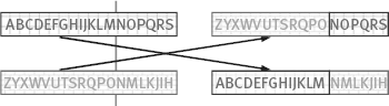
There are many ways for realizing crossover, the basic idea is randomly to match pairs of the new generated code string to determine the location of border for each pair of random code strings, and to generate new code strings by exchange of the heads of string pairs and the location of border, as shown in Figure 5.8.

Not all newly generated code strings should cross. Generally a probability parameter is used to control the required number of cross-code string. Another method is to make the best copy of code string retain its original form.

5.3.1.3Mutation

The principle of mutation operation is to frequently and randomly change some codes in a code string (e. g., making a change for every one of a thousand codes in the evolution from one generation to the next generation), in order to maintain a variety of local structures to avoid losing some optimal characteristics of solutions.

The convergence of the genetic algorithms is worthy of attention. It plays an important role in controlling whether the evolution should be stopped. In practice, if the group with largest fitness was no significant increase in several processes of evolution, then it can be stopped.

5.3.1.4Algorithm Steps

According to the above three basic operations, the genetic algorithms consist of the following steps:

(1)Generating encoded string for initial population, giving objective function value (fitness)

(2)Coping code strings with high fitness (according to probability) in the new group of populations, removing code strings with low fitness

(3)Building a new code string from the encoded strings copied from the old populations through cross combination

(4)Occasionally, making mutation of a code randomly selected from code strings

(5)Ranking the code strings of the current population, according to their fitness

(6)If the fitness values of the code string with maximum fitness are not significantly increased in several evolutionary processes, stop; otherwise, return to step 2 to continue the calculation

5.3.2Semantic Segmentation and Interpretation

An important feature of the genetic algorithm is to consider all the samples of population groups in a single process step, the samples with a high degree of adaptation will be retained and others will die. This feature is suitable for semantic image segmentation. Here the semantic segmentation refers to divide the image into regions based on the semantic information and optimizing the results according to the context and other high-level information.

5.3.2.1Objective Function

The image interpretation using genetic algorithm is based on the principle of hypothesis testing, where the objective functions optimized by genetic algorithm evaluate the quality of image segmentation and semantic interpretation. Algorithms begin with an over-segmented image (called the primary segmentation), the start region in this over-segmented image is called the primary region. Algorithm constantly and iteratively updates and merges the primary region into the current regional, namely continuous building viable region division and interpreting new assumption samples.

The primary region available can be described by using the primary region adjacency graph. The combination of primary region adjacency graphs can produce a specific region adjacency graph. Specific region adjacency graph can express the region merged from all the adjacency regions with the same interpretation. Each possible semantic image segmentation corresponds to only one particular region adjacency graph. Specific region adjacency graph can be used to evaluate the objective function of semantic segmentation.

The design of an objective function (i.e., the fitness function in genetic algorithm) is a key issue of semantic segmentation. This function must be based on the property of image regions and relationship among these regions, in which the utilization of a priori knowledge of the desired segmentation is required. The optimization of objective function consists of three parts:

(1)The confidence that is proportional to corresponding probability in interpretation ki for region Ri, according to the nature of the region itself, is

$C\left(k_i|X_i\right)\text{oc}P\left(k_i|X_i\right)\left(5.11\right)$

wherein C(ki) can be computed according to eq. (5.12), NR is the number of regions in the corresponding specific region adjacency graph. Genetic algorithms try to optimize the objective function Cimage representing the current segmentation and interpretation hypothesis.

Segmentation optimization function is based on unary properties of hypothesized regions and on binary relations between these regions and their interpretations. In the evaluation of local region confidence C(ki|Xi), a priori knowledge about the characteristics of the image under consideration is used.

5.3.2.2Concrete Steps and Examples

According to the objective function described above, the procedure using genetic algorithm for segmentation and semantic interpretation has the following steps

(1)Initializing the original image into primary region, the corresponding relationship between the relative position of each region and its label in genetic algorithm generated code string is defined.

(2)Building a primary region adjacency graph.

(3)Selecting the starting population of code string at random. Whenever possible, it is better to use a priori knowledge for determining the starting population.

(4)Genetic optimization of the current population, with the help of the current region adjacency graph to compute the value of optimal segmentation function for each code string.

(5)If the maximum value of optimization criteria did not change significantly in a number of successive steps, go to step 7.

(6)Let genetic algorithm generate a new population with assumptions on segmentation and interpretation, go to step 4.

(7)The final obtained code string that has the greatest confidence (optimal segmentation hypothesis) represents the ultimate semantic segmentation and interpretation.

Example 5.1 Semantic segmentation example

One synthetic image and its graph representations are shown in Figure 5.9. Figure 5.9(a) represents a scene image with a ball on the grass, Sonka (2008). Preliminary semantic segmentation divided it into five different regions Ri, i = 1 ~ 5, abbreviated 1 ~ 5 in the figure. Figure 5.9(b) gives the region adjacency graph of Figure 5.9(a), in which nodes represent regions, and arcs connect nodes of adjacent regions. Figure 5.9(c) shows the dual graph of Figure 5.9(b), where nodes correspond to the intersection of different regional contours, and arcs correspond to the contour segment.

Let B represent the marker for the ball, L represent the marker for the grass. High-level knowledge used is: the image has a round ball that is in the green grass region. Define two unary conditions: one is the confidence that a region in a ball region depends on the compactness of region C

$C\left(k_i=B|X_i\right)=\text{compactness}\left(R_i\right)\left(5.15\right)$

and another is the confidence that a region in a grassland region depends on the greenness of region G

$C\left(k_i=L|X_i\right)=\text{greenness}\left(R_i\right)\left(5.16\right)$

Suppose that the confidence of region constituted by ideal sphere ball and the confidence of region constituted by ideal lawn area are both equal to 1, that is

$\begin{array}{l}C\left(B|\text{circular}\right)=1\left(5.17\right)\\ C\left(L|\text{green}\right)=1\end{array}$

Define a binary condition: the confidence that a region is inside another region is provided by the following compatibility function

$r\left(B|\text{is}\text{inside}L\right)=1\left(5.18\right)$

The confidences of other combinations are zero.

Unary conditions show that the more compact a region, the more round it is, and the higher it is interpreted as a sphere. Binary condition indicates that a ball can only be completely surrounded by a lawn.

Let the code strings represent the region labels in order of region numbers, that is, the region numbers correspond to the location of region labels in the code string. Suppose at random the code strings obtained by region labeling are BLBLB and LLLBL, which represent the two groups of segmentation hypotheses shown in Figure 5.10. In each group of Figure 5.10, the left figure is the interpretation, the up-right is the corresponding code string, and the low-right is the corresponding region adjacency graph.

Suppose a randomized crossover is performed at the location| between the second position and third position (represented by |). According to eq. (5.13), the respective confidences of compactness representing ball region and of location that the ball region is inside grassland are as follows: $BL|BLB\Rightarrow C_{\text{image}}=0.00,LL|LBL\Rightarrow C_{\text{image}}=$ $0.12,LLBLB\Rightarrow C_{\text{image}}=0.20,BLLBL\Rightarrow C_{image}=\mathrm{0.00.}$ The latter two code strings are obtained by swapping the parts before | in the former two code strings, as shown in Figure 5.11.

From the above confidence values, it is seen that the second and third segmentation hypotheses corresponding to the second and third code strings are relatively the best. Therefore, the first and four code strings can be eliminated, while for the second and third code strings another randomized crossover between the third position and fourth position can be conducted. The new confidences are as follows: LLL|BL Cimage = 0.12, LLB|LB Cimage = 0.20, LLLLB Cimage = 0.14, LLBBL Cimage = 0.18. The latter two code strings are obtained by swapping the parts after in the former two code strings.

Now, selecting the aforementioned second and fourth code strings, another randomized crossover is performed at the location between the fourth position and fifth position. The new confidences are as follows: LLBLB Cimage = 0.20, LLBBL Cimage = 0.18, LLBLL Cimage = 0.10, LLBBB Cimage = 1.00. The latter two code strings are obtained by swapping the parts after | in the former two code strings. Because the current code string LLBBB has the highest degree of confidence among available segmentation hypotheses, so genetic algorithm stops. In other words, if it continues to generate hypotheses, no better confidence would be obtained. Thus the obtained optimal segmentation result is shown in Figure 5.12.

5.4Labeling of Objects in Scene

Labeling objects in scene refers to the semantic labeling of object regions in image, that is, to assign the semantic symbols to objects. Here, it is assumed that regions corresponding to the image of scene have been detected, and the relationship between these regions and objects has been described by the region adjacency graph or by the semantic web. The property of the object itself can be described by unary relationship, while the relationship among objects can be described by binary or higher-order correlations. The objective of labeling objects in scene is to assign a tag (with semantic meaning) for each object in the image of scene so as to obtain the proper interpretation of the scene image. Thus obtained interpretation should be consistent with the scene knowledge. Tags need to have consistency (i.e., any two objects in image are in reasonable structure or relationship), and tend to have the most likely explanation when there are multiple possibilities.

5.4.1Labeling Methods and Key Elements

For the labeling of objects in scene, there are mainly two methods, Sonka (2008).

(1)Discrete labeling. It assigns each object just a tag, the main consideration is the consistency of the image tags.

(2)Probabilistic labeling. It allows assigning multiple tags to the jointly existing objects. These tags are weighted by the probability, and each tag has a confidence.

The difference between the two methods is mainly reflected in the robustness of the scene interpretation. There are two results for discrete tag, one is that a consistent tag is obtained, the other is that the impossibility of assigning a consistent tag to scene is detected. Due to the imperfection of segmentation, discrete tag will generally give the result that is not consistent in description (even if only a few local inconsistencies were detected). On the other hand, the probability tag can always give the labeling results and corresponding trusts. Although it is possible to have some locally inconsistent results, which are still better than the description results provided by discrete tag, which are consistent but quite impossible. In extreme cases the discrete tag can be regarded as a special case of the probability tag, in which the probability of one tag is 1 and the probabilities of all other tags are 0.

The method of scene labeling includes the following key elements:

(1)A group of objects Ri, i = 1,2,..., N;

(2)For each object Ri, there is a limited set of tags Qi, this same set is also applicable to all objects;

(3)A limited set of relationship between objects;

(4)A compatibility function between related objects. This reflects the constraints for relationship between objects.

If the direct relationship among all objects in image should be considered for solving labeling problems, a very large amount of computation is required. Therefore, the method of constraint propagation is generally used. That is, the local constraint is used to obtain local consistency (the local optimum), then the iterative method is used to adjust the local consistency to the global consistency of the entire image (the global optimum).

5.4.2Discrete Relaxation Labeling

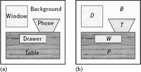
One example for scene labeling is shown in Figure 5.13. Figure 5.13(a) shows a scene with five object regions (including the background), Sonka (2008). The five regions are denoted by B (background), W (window), T (table), D (drawer) and P (phone). Unary properties for describing objects are:

(1)The windows are rectangular;

(2)The table is rectangular;

(3)The drawer is rectangular.

Binary constraints/conditions are as follows:

(1)The windows are located above the table;

(2)The phone is on the table;

(3)The drawer is inside the table;

(4)The background is connected with image boundary.

Under these constraints, some of the results in Figure 5.13(b) are not consistent.

An example of a discrete relaxation labeling process is shown in Figure 5.14. First, all existing tags are assigned to each object, as shown in Figure 5.14(a). Then, the iterative checking of the consistency is performed for each object to remove those tags that is likely to not satisfy the constraints. For example, considering the connection of background and the boundary of the image could determine the background in the beginning, and subsequently the other objects could not be labeled as background. After removing the inconsistent tags, Figure 5.14(b) will be obtained. Then considering that the windows, tables, and drawers are rectangular, the phone can be determined, as shown in Figure 5.14(c). Proceeded in this way, the final consistency results with correct tags are shown in Figure 5.14(d).

5.4.3Probabilistic Relaxation Labeling

As a bottom-up method for interpretation, discrete relaxation labeling may encounter difficulties when the object segmentation was incomplete or incorrect. Probabilistic relaxation labeling method may overcome the problem of object loss (or damage) and the problem of false object, but may also produce certain ambiguous inconsistent interpretations.

Considering the local structure shown on the left of Figure 5.15, its region adjacency graph is on the right part. The object Rj is denoted qj, qj Q, Q = {w1, w2,..., wT}.

The compatibility function of two objects Ri and Ri with respective tags qi and qj is r(qi = wk, qi = wl). The algorithm iteratively searches the best local consistency in whole image. Suppose in step b of iterative process the tag qi is obtained according to the binary relationship of Ri and Rj, then the support (wk for qi) can be expressed as

$S_j^{\left(b\right)}\left(q_i=w_k\right)={\displaystyle \sum _{l=1}^{T}r\left(q_1=w_k,q_j=w_l\right)P^{\left(b\right)}\left(q_j=w_l\right)}\left(5.19\right)$

where P(b)(qj = wl) is the probability that the region Rj is labeled as wl at this time. Consider all the N objects Rj (labeled with wj) linked with Ri (labeled with wj), the total support obtained is

$S^{\left(b\right)}\left(q_l=w_k\right)={\displaystyle \sum _{j=1}^N{C}_{ij}{S}_j^{\left(b\right)}}\left(q_l=w_k\right)={\displaystyle \sum _{j=1}^N{C}_{ij}}{\displaystyle \sum _{l=1}^{T}r\left(q_i=w_k,q_j=w_l\right)}{P}^{\left(b\right)}\left(q_j=w_l\right)\left(5.20\right)$

where cij is a positive weight to meet ${\displaystyle \sum {}_{j-1}^N{c}_{ij}=1,}$ which represents the binary contact strength between two objects Ri and Rj. The iterative update rule is

$P^{\left(b+1\right)}\left(q_i=w_k\right)=\frac{1}{K}{P}^{\left(b\right)}\left(q_i=w_k\right)S^{\left(b\right)}\left(q_i=w_k\right)\left(5.21\right)$

where K is the normalization constant:

$K={\displaystyle \sum _{l=1}^T{P}^{\left(b\right)}\left(q_i=w_l\right)S^{\left(b\right)}\left(q_l=w_l\right)}$