To match Rl and Rr, a corresponding transform, which yields the minimum error (counted by number of errors) between Rl and Rr, needs to be searched. Note that E is a function of p, so the transform p looked for should satisfy

${\text{dis}}^c\left(R_{\text{1}},R_{\text{r}}\right)=\underset{p}{\inf }\left\{{\displaystyle \sum _i{W}_{i}C}\left[E_i\left(p\right)\right]\right\}\left(4.30\right)$

Referring back to eqs. (4.21) and (4.22), to match two relations sets X, and Xr, a set of transforms pj should be found, which make the following equation valid

${\text{dis}}^c\left(X_1,X_r\right)=\underset{p}{\inf }\left\{{\displaystyle \sum _j^m{V}_j{\displaystyle \sum _i^{}{W}_{ij}c\left[E_{ij}\left(p_j\right)\right]}}\right\}\left(4.31\right)$

In eq. (4.31), it is assumed that n > m, where Vj are the weights for counting the different importance of relations.

Example 4.2 Matching of connection relations.

Consider the case of matching two objects in Example 4.1 only using connection relations. From eqs. (4.23) and (4.24), it has

$\begin{array}{l}{R}_1=\left[\left(A,B\right)\left(A,C\right)\right]=S\left(1\right)\times S\left(2\right)\subseteq S^M\\ R_{\text{r}}=\left[\left(1,2\right)\left(1,3\right)\left(1,4\right)\left(2,4\right)\left(3,4\right)\right]=T\left(1\right)\times T\left(2\right)\times T\left(3\right)\times T\left(4\right)\times T\left(5\right)\subseteq T^N.\end{array}$

When there is no component 4 in Qr, Rr = [(1,2)(1,3)]. In this case, p = {(A,1) (B, 2)(C, 3)}, p−1 = {(1, A)(2, B)(3, C)}, Rl ⊕ p = {(1,2)(1,3)}, and Rr ⊕ p = {(A, B)(A, C)}. The four errors in eq. (4.27) are

$\begin{array}{l}{E}_1=\{R_1\oplus p-\left(R_1\oplus p\right)\cap R_r\}=\{\left(1,2\right)\left(1,3\right)=\{\left(1,2\right)\left(1,3\right)\}=0\\ E_2=\{R_r-R_r\cap \left(R\oplus p\right)\}=\left\{\left(1,2\right)\left(1,3\right)\right\}-\left\{\left(1,2\right)\left(1,3\right)\right\}=0\\ E_3=\{R_r\oplus p^{-1}-(R_r\oplus p^{-1})\cap R_1\}=\left\{\left(A,B\right)\left(A,C\right)\right\}=0\\ E_4=\{R_1-R_1\cap \left(R_r\oplus p^{-1}\right)\}=\left\{\left(A,B\right)\left(A,C\right)\right\}-\left\{\left(A,B\right)\left(A,C\right)\right\}=0\end{array}$

It is evident that dis(Rl, Rr) = 0. When there is the component 4 in Qr, Rr = [(1,2)(1,3) (1,4)(2,4)(3,4)]. In this case, p = {(A,4)(B,2)(C,3)}, p−1 = {(4, A)(2, B)(3, C)}, Rl ⊕ p = {(4,2)(4,3)}, and Rr ⊕ p = {(B, A)(C, A)}. The four errors in eq. (4.27) become

$\begin{array}{l}{E}_1=\left\{\left(4,2\right)\left(4,3\right)\right\}-\left\{\left(4,2\right)\left(4,3\right)\right\}=0\\ E_2=\left\{\left(1,2\right)\left(1,3\right)\left(1,4\right)\left(2,4\right)\left(3,4\right)\right\}=\left\{\left(2,4\right)\left(3,4\right)\right\}=\left\{\left(1,2\right)\left(1,3\right)\left(1,4\right)\right\}\\ E_3=\left\{\left(B,A\right)\left(C,A\right)\right\}-\left\{\left(A,B\right)\left(A,C\right)\right\}=0\\ E_4=\left\{\left(A,B\right)\left(A,C\right)\right\}-\left\{\left(A,B\right)\left(A,C\right)\right\}=0\end{array}$

If only the connection relation is considered, the order of components in the expression can be exchanged. From the above results, dis(Rl, Rr) = {(1,2)(1,3)(1,4)}. The numbers of errors are C(E1) = 0, C(E2), = 3, C(E3), = 0, C(E4), = 0. Finally, disC(Rl, Rr) =3.

Matching uses the model stored in the computer to recognize the unknown pattern of the object to be matched. Once a set of transforms pj are obtained, their corresponding models should be determined. Suppose that the object to be matched X is defined in eq. (4.21). For each of a set of models Y1, Y2,..., YL (they can be represented by eq. (4.22)), a set of transforms p1, p2, ..., pL can be found to satisfy the corresponding relation in eq. (4.31). In other words, all distance disC(X, Yq) between X and the set of models can be obtained. If for a model Yq, its distance to X satisfies

${\text{dis}}^c\left(X,Y_q\right)=\min \left\{{\text{dis}}^c\left(X,Y_i\right)\right\}i=1,2,\cdot \cdot \cdot ,L\left(4.32\right)$

for q ≤ L, it has X Yq. This means that X can be matched to the model Yq.

In summary, the whole matching process has four steps.

(1)Determining the relations among components (i.e., for a relation given in Xl, determine the same relation in Xr). This requires m × n comparisons

(2)Determining the transform for the matching relations; that is, determine p to satisfy eq. (4.30). Suppose that p has K possible forms. The task is to find, among K transforms, the one providing the minimum value for the weighted error summation.

$R_{\text{l}}\left\{\begin{array}{l}\underrightarrow{p_1:{\text{dis}}^C\left(R_1,R_{\text{r}}\right)}\\ \underrightarrow{p_2:{\text{dis}}^C\left(R_1,R_{\text{r}}\right)}\\ \mathrm{......}\\ \underrightarrow{p_k:{\text{dis}}^C\left(R_1,R_{\text{r}}\right)}\end{array}\right\}{R}_{\text{r}}$

(4)Determining the model (find the minimum in L disC(Xl, Xr))

$X\{\begin{array}{l}\underrightarrow{p_1}{Y}_1\to {\text{dis}}^C\left(X,Y_1\right)\\ \underrightarrow{p_2}{Y}_2\to {\text{dis}}^C\left(X,Y_2\right)\\ \mathrm{.........}\\ \underrightarrow{p_L}{Y}_L\to {\text{dis}}^C\left(X,Y_L\right)\end{array}\left(4.36\right)$

4.5Graph Isomorphis

A graph is a data structure used for describing relations. A graph isomorphism is also a technique for matching relations. In the following, some fundamental definitions and concepts about the graph theory are first introduced, and then the graph isomorphic technique is discussed.

4.5.1Fundamentals of the Graph Theory

Some basic concepts, definitions, and representations of graphs are given first.

4.5.1.1Basic Definitions

In Graph theory, a graph G is defined by a limit and nonempty vertex set V(G) and a limit edge set E(G), which can be denoted

$G=\left[V\left(G\right),E\left(G\right)\right]=\left[V,E\right]\left(4.37\right)$

where every element in E(G), called a no-order edge, corresponds to a pair of vertexes.

It is common to denote the elements in set V by capital letters and the elements in set E by small letters. The edge e formed by vertex pairs A and B is denoted e $\leftrightarrow$ AB or e BA. Both A and B are the ends of e, or e joins A and B. In this case, vertexes A and B are incident with edge e, and edge e is incident with vertexes A and B. Two vertexes incident with the same edge are adjacent. Similarly, two edges incident with the same vertex are adjacent. If two edges have two same vertexes, they are called multiple edges or parallel edges. If the two vertexes of an edge are the same one, this edge is called a loop; otherwise, this edge is called a link.

In the definition of a graph, two vertexes may be the same or may be different, while two edges may be the same or may be different, too. Different elements can be represented by vertexes with different colors. This is called the color property of vertexes. Different relations between elements can be represented by edges with different colors. This is called the color property of edges. A general/extended color graph G is denoted

$G=\left[\left(V,C\right)\left(E,S\right)\right]\left(4.38\right)$

where V is a vertex set, C is the color property set of vertexes, E is an edge set and S is the color property set of edges

$V=\left\{V_1,V_2,\mathrm{...},V_N\right\}\left(4.39\right)$

$C=\left\{C_{V_1},C_{V_2},\mathrm{...},C_{V_N}\right\}\left(4.40\right)$

$E=\left\{e_{V_1{V}_j}|V_i,V_j\in V\right\}\left(4.41\right)$

$S=\left\{S_{V_i{V}_j}|V_i,V_j\in V\right\}\left(4.42\right)$

4.5.1.2Geometric Representation of Graphs

Denote the vertexes of a graph by round points and the edges of a graph by lines or curves connecting vertexes. A geometric representation or geometric realization of a graph can be obtained. For the graph with the number of edges larger than 1, there may be infinite numbers of geometric representations.

Example 4.3 Geometric representation of a graph.

Suppose that V(G) = {A, B, C}, E(G) = {a, b, c, d}, where a $\leftrightarrow$ AB, b AB, c BC, and d CC. This graph can be represented by Figure 4.8.

In Figure 4.8, edges a, b, and c are adjacent to each other, and edges c and d are adjacent, but edges a and b are not adjacent to edge d. Similarly, vertexes A and B are adjacent, and vertexes B and C are adjacent, but vertexes A and C are not adjacent. Edges a and b are multiple edges, edge d is a loop, and edges a, b, and c are links.

Example 4.4 Illustrations of color graph representation.

The two objects in Example 3 can be represented by the two graphs in Figure 4.9, where the color properties of vertexes are distinguished by different vertex forms and the color properties of edges are distinguished by different line types.

4.5.1.3Subgraph

For two graphs G and H, if V(H) ⊆ V(G) and E(H) ⊆ E(G), graph H is called the subgraph of graph G, and this is denoted by H ⊆ G. On the other hand, graph G is called the super-graph of graph H. If graph H is the subgraph of graph G, but H ≠ G, graph H is called the proper subgraph of graph G, and graph G is called the proper super-graph of graph H, Sun (2004).

If H ⊆ G and V(H) = V(G), graph H is called the spanning subgraph of graph G, and graph G is called the proper super-graph of graph H. For example, Figure 4.10(a) shows graph G, while Figure 4.10(b–d) represents different spanning subgraphs of graph G.

By removing all multiple edges and loops from graph G, a simple spanning subgraph can be obtained. This subgraph is called the underlying simple graph of graph G. Among three spanning subgraphs shown in Figure 4.10(b–d), there is only one underlying simple graph; that is, Figure 4.10(d).

In the following, graph G in Figure 4.11(a) is used to show four operations for obtaining the underlying simple graph.

(1)For a nonempty vertex subset V′(G) ⊆ V(G) in graph G, if one of the subgraphs of graph G takes V′(G) as the vertex set and takes all edges with two ends in V′(G) as the edge set, this subgraph is called an induced subgraph of graph G. It can be denoted as G[V′(G)] or G[V′]. Figure 4.11(b) shows G[A, B, C] = G[a, b, c].

(2)For a nonempty edge subset E′(G) ⊆ E(G) in graph G, if one of the subgraphs of graph G takes E′(G) as the edge set and takes vertexes of all edges in graph G as the vertex set, this subgraph is called an edge-induced subgraph of graph G. It can be denoted as G[E′(G)] or G[E′]. Figure 4.11(c) shows G[a, d] = G[A, B, D].

(3)For a nonempty vertex proper subset V′(G) ⊆ V(G) in graph G, a subgraph of graph G is also called an induced subgraph of graph G if the following two conditions are satisfied. The first condition is that this subgraph take all vertexes, except those in V′(G) ⊂ V(G), as its vertex set. The second condition is that this subgraph take all edges, except those in relation with V′(G), as its edge set. Such a subgraph is denoted G − V′. It has G − V′ = G[VV′]. Figure 4.11(d) shows G − {A, D} = G[B, C] = G[{A, B, C, D} − {A, D}].

(4)For a nonempty edge proper subset E′(G) ⊆ E(G) in graph G, if one of the subgraphs of graph G takes the rest of the edges after removing the edges in E′(G) ⊂ E(G) as the edge set, this subgraph is also called an induced subgraph of graph G, which can be denoted G − E′. Note that G − E′ and G[EE′] have the same edge set, but they are not always identical. The former is always a spanning subgraph while the latter may not be. Figure 4.11(e) shows an example of the former, G − {c} = G[a, b, d, e]. Figure 4.11(f) shows an example of the latter, G[{a, b, c, d, e} − {a, b}] = G − A ≠ G − [{a, b}].

4.5.2Graph Isomorphism and Matching

Based on the above described concepts, a graph isomorphism can be identified and graph matching can be performed.

4.5.2.1Identical Graphs and Graph Isomorphic

According to the definition of graph, if and only if two graphs G and H satisfy V(G) = V(H) and E(G) = E(H), they are called identical graphs and can be expressed by the same geometric representations. For example, graphs G and H in Figure 4.12 are identical and expressed by the same geometric representations. However, if two graphs can be expressed by the same geometric representations, they are not necessarily identical. For example, graphs G and I in Figure 4.12 are not identical though they can be expressed by the same form of geometric representation.

For two graphs expressed by the same geometric representations but that are not identical, if the labels of the vertexes and/or the edges of one graph are changed, it is possible to make it identical to another graph. In this case, these two graphs can be called isomorphic. In other words, the isomorphism of two graphs means that there are one-to-one correspondences between the vertexes and edges of the two graphs. Two isomorphic graphs G and H can be denoted G ≅ H. The sufficient and necessary conditions for two graphs G and H to be isomorphic are given by

$P:V\left(G\right)\to V\left(H\right)\left(4.43\right)$

$Q:E\left(G\right)E\left(H\right)\left(4.44\right)$

Mappings P and Q have the relation of Q(e) = P(u)P(v), as shown in Figure 4.13.

4.5.2.2Determination of Isomorphism

According to the above discussion, isomorphic graphs have the same structures and the differences are the labels of the vertex and/or edge. Some examples are discussed here. For simplicity, assume that all vertexes have the same color properties and all edges have the same color properties. Consider a single color graph (a special case of G)

$B=\left[\left(V\right)\left(E\right)\right]\left(4.45\right)$

where V and E are given by eqs. (4.39) and (4.41), respectively. The difference is that all elements in each set are the same here. With reference to Figure 4.14, suppose that two graphs B1 = [(V1)(E1)] and B2 = [(V2)(E2)] are given. Matching using graph isomorphism has the following forms, Ballard (1982).

Graph Isomorphism

Graph isomorphism is a one-to-one mapping between B1 and B2. For example, Figure 4.14(a, b) represents graph isomorphism. In general, denote f as a mapping, and for e1 E1 and e2 E2, there must be f(e1) = e2. In addition, for each edge of E1 connecting any pair of vertexes e1 and ${e^{\prime }}_1\left(e_1,{e^{\prime }}_1\in E_1\right),$ there must be an edge of E2 connecting f(e1) and $f\left({e^{\prime }}_1\right).$

Subgraph Isomorphism

Subgraph isomorphism is a type of isomorphism between a subgraph of B1 and the whole graph of B2. For example, several subgraphs in Figure 4.14(c) are isomorphic with Figure 4.14(a).

Double-subgraph Isomorphism

Double-subgraph isomorphism is a type of isomorphism between every subgraph of B1 and every subgraph of B2. For example, there are several double subgraphs in Figure 4.14(d), which are isomorphic with Figure 4.14(a).

One method that is less restrictive than the isomorphism and faster in convergence is to use the association graphs for matching, Snyder (2004). In matching with the association graph, a graph is defined as G = (V, P, R), where V represents a set of vertexes, P represents a set of unary predicates on vertexes, and R represents binary relations between vertexes. A predicate takes on only the value of TRUE or FALSE. A binary relation describes a property possessed by a pair of vertexes. Given two graphs, an association graph can be constructed. Matching using association graphs is to match the vertexes and the binary relations in two graphs.

4.6Labeling of Line Drawings

In a 3-D world, the surfaces of 3-D objects could be observed. Projecting a 3-D world onto a 2-D image, each surface will form a region. The boundary of surfaces in the 3-D world becomes the contour of the regions in the 2-D image. Line drawings are the result of representing the object regions by their contours. For simple objects, by labeling their line drawings, (i.e., by using contour labels of 2-D images) the relationship among 3-D surfaces can be represented, Shapiro (2001). Such a label can be used to match 3-D objects and their models for interpreting the scene.

4.6.1Labeling of Contours

Some commonly used terms in labeling of contours are as follows:

(1)Blade
If a continuous surface (occluding surface) occludes another surface (occluded surface), when it goes along the contour of the former surface, the change of the surface normal direction would be smooth and continuous. In this case, the contour is called a blade. To represent a blade on line drawings, a single arrowhead “>” is used. The direction of the arrow is used to indicate which surface is the occluding surface. By convention, the occluding surface is located to the right side of blade as the blade is followed in the direction of the arrow. In two sides of a blade, the directions of the occluding surface and the occluded surface have no relation.

(2)Limb
If a continuous surface occludes not only another surface but also part of itself (self-occluding), the change of the surface normal direction is smooth and continuous, and this change is perpendicular to the viewing direction, then the contour line is called a limb. To represent a limb, two opposite arrows “< >” are used. Following in the direction of the arrow, the surface directions are not changed. Following the direction that is not parallel to a limb, the surface direction changes continuously.
A blade is a real edge of a 3-D object, but a limb is not. Both the blade and the limb belong to jump edges. In the two sides of a jump edge, the depth is not continuous.

(3)Crease
If an abrupt change to a 3-D surface or the joining of two different surfaces is encountered, a crease is formed. In the two sides of a crease, the points on the surface are continuous, but the surface normal directions are not continuous. If the surface is convex at the crease place, it is marked by a “+” symbol. If the surface is concave at the crease place, it is marked by a “−” symbol.

(4)Mark
The mark of an image contour is caused by a change in the surface albedo. A mark is not caused by the 3-D surface shape. A mark can be labeled “M.”

(5)Shade
If a continuous surface does not occlude another surface or part of another surface along the viewing direction, but does occlude the illumination of light source for another surface or part of another surface, it will cause shading in the second surface. The shading on the surface is not caused by the form of the surface, but is caused by the influence of other parts of the surface. A shade can be labeled “S.”

Example 4.5 Examples of contour labeling.

Some examples of contour labeling are illustrated in Figure 4.15. In Figure 4.15, a hollow cylinder is put on a platform, there is a mark on the cylinder, and the cylinder forms shading on the platform. There are two limbs on the two sides of the cylinder. The top edges are divided into two parts by two limbs. The top-front (edge) represents a blade that occludes the platform while the bottom-front (edge) represents a surface that occludes the interior of the cylinder. All creases on the platform are convex, while the crease between the cylinder and the platform is concave.

4.6.2Structure Reasoning

In the following, structure reasoning for 3-D objects is based on their contours in 2-D images. Suppose that all surfaces of an object are planes and all corners are formed by the cross of three planes. Such a 3-D object is called the trihedral corner object. Two line drawing examples of the trihedral corner object are shown in Figure 4.16. In Figure 4.16, both objects are in a general position, which means that a small change of viewpoint will not cause the topological change of the line drawing (no face, edge or connection will disappear) at such a position.

The two line drawings in Figure 4.16 are the same in geometric structure. However, two different interpretations can be derived. The difference between these line drawings is the three additional concave creases in the line drawing of Figure 4.16(b). Therefore, the object in Figure 4.16(a) is viewed as floating in the space and the object in Figure 4.16(b) is viewed as glued to a back wall.

To label the line drawing, three labels {+, −, →} can be used, in which “+” represents a nonclosed convex line, “−” represents a nonclosed concave line and “→” represents a closed line. Under these conditions, there are four possible groups of 16 types of topological combinations of line junctions. That is, there are six types of L-junctions, four types of T-junctions, three types of arrows, and three types of forks (Y-junction), as shown in Figure 4.17. Note that other topological combinations do not physically exist.

4.6.3Labeling with Sequential Backtracking

There are different methods for automatic labeling of line drawings. In the following, a method called labeling with sequential backtracking is introduced, Shapiro (2001). The problem to be solved can be stated easily. Given a 2-D line drawing with a set of edges, assign each edge a label (the junctions used are shown in Figure 4.17) to interpret the 3-D cause. The method of labeling with sequential backtracking arranges edges into a sequence. If possible, the edges with the most constrained labels should be assigned first. According to the depth first strategy, each edge is labeled with all possible labels and the consistency of the new label with other edge labels is checked. If a newly assigned label produces a junction that is not in the junction types shown in Figure 4.17, then backtrack; otherwise, try the next edge. If all labels are consistent, a label result is obtained and a complete path to the leaves is found.

Example 4.6 Illustration of labeling with sequential backtracking.

Considering the pyramid with four faces shown in Figure 4.18, the interpretation tree obtained by labeling with sequential backtracking, including each step and the result, is shown in Table 4.1.

It is seen from the interpretation tree that three complete paths can be obtained. They give three different interpretations of a line drawing.

4.7Problems and Questions

4-1What is the relation between template matching and the Hough transform? Q Compare their computation expense when detecting points on a line.

4-2*Show that Q in eq. (4.11) is 0 if and only if A and B are identical strings.

4-3Show that the translation, rotation, and scaling parameters discussed in Section 4.2 can be computed independently.

4-4When constructing dynamic patterns, what relations, except connecting line lengths and their angles, can still be used? Give the expressions for pattern vectors.

4-5Considering only the connecting relation, compute the distances between the object in the right side of Figure 4.7 and the two objects in Figure Problem 4-5, respectively.

Figure Problem 4-5

4-6Show that if two graphs are identical, then the numbers of the vertex and edge in the two graphs are equal. However, if the numbers of vertex and edge in two graphs are equal, these two graphs may not be identical.

4-7*Show that the two graphs in Figure Problem 4-7 are not isomorphic.

Figure Problem 4-7

4-8Provide all subgraphs in Figure 4.14(c), which are isomorphic with Figure 4.14(a).

4-9Draw the 16 subgraphs that have {A, B, C, D} as vertex sets in Figure Problem 4-3.

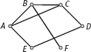
Figure Problem 4-9

4-10How do you distinguish a blade from a limb using shading analysis?

4-11List the junction types (see Figure 4.17) of all junctions for the two objects in Figure 4.16.

4-12Design a line drawing that corresponds to a nonexist object.

4.8Further Reading

1.Fundamental of Matching

–Many matching techniques use Hough transforms, such as the general Hough transform, Chen (2001), the iterative Hough transform (IHT), (Habib 2001), and the multi-resolution Hough transform, Li (2005a).

2.Object Matching

–Several modified Hausdorff distances have been proposed, see Gao (2002b), Lin (2003), Liu (2005), and Tan (2006).

–One method for combining curve fitting and matching for tracking of infrared objects can be found in Qin (2003).

3.Dynamic Pattern Matching

–Examples of utilization of dynamic pattern matching in bio-medical image analysis can be found in Zhang (1991).

–A method similar to dynamic pattern matching, called a local-feature-focus algorithm, is discussed in Shapiro (2001).

4.Relation Matching

–Relation is a general concept, and relation matching can have many different forms; for example, see Dai (2005).

–Relation matching has been popularly used in content-based visual information retrieval, Zhang (2003b).

5.Graph Isomorphism

–A more detailed introduction to graph theory can be found in Marchand (2000), West (2001), Buckley (2003), and Sun (2004).

–Double-subgraph isomorphism has a big search space. It can be solved with the help of another graph method for cliques, Ballard (1982).

6.Labeling of Line Drawings

–The labeling of line drawings gets help from the graph theory, so further reading can be found in Marchand (2000), Sun (2004), and so on.