3.3Shape from Shading

In contrast to the techniques in photometric stereo and structure from motion that need to at least capture two images of a scene, the technique of shape from shading can recover the shape information of a 3-D scene from a single image.

3.3.1Shading and Shape

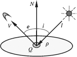
When an object is illuminated in a scene, different parts of its surface will appear with different brightness, as they are oriented differently. This spatial variation of brightness is referred to as shading. The shading on an image depends on four factors: The geometry of the visible surface (surface normal), the radiance direction and radiance energy, the relative orientation and distance between an object and an observer, and the reflectance property of the object surface, Zhang (2000b). The meaning of the letters in Figure 3.23 is as follows. The object is represented by the patch Q, and the surface normal N indicates the orientation of the patch. The vector I represents the incidence intensity and the direction of the source. The vector V indicates the relative orientation and distance between the object and the observer. The reflectance property of the object surface p depends on the material of the surface, which is normally a scale, but can be the function of the patch’s spatial position.

According to Figure 3.23, the image’s gray levels depend on the incidence intensity I, the reflectance property of the object surface ρ, and the angle between the viewing direction and the surface normal i, which is given by

$E\left(x,y\right)=I\left(x,y\right)\rho \cos i\left(3.80\right)$

Consider the case where the light source is just behind the observer, cos i = cos e. Suppose that the object has a Lambertian surface; that is, the surface reflectance intensities are not changed with the observation locations. The observed light intensities are

$E\left(x,y\right)=I\left(x,y\right)\rho \cos e\left(3.81\right)$

Since N = [pq – 1]T and V = [0 0 – 1]T, by overlapping the gradient coordinate system onto the XY coordinate system, as shown in Figure 3.24,

$\cos e=\cos i=\frac{{\left[pq-1\right]}^T•{\left[00-1\right]}^T}{{\left[pq-1\right]}^T|•|{\left[00-1\right]}^T|}=\frac{1}{\sqrt{\left(p^2+q^2+1\right)}}\left(3.82\right)$

Taking eq. (3.82) into eq. (3.80) yields

$E\left(x,y\right)=I\left(x,y\right)\rho \frac{1}{\sqrt{p^2+q^2+1}}\left(3.83\right)$

Consider now the case where i = e, and suppose that I is perpendicular to the patch Q, which has a normal [pi qi − 1]T. Then it has

$\cos i=\frac{{\left[pq-1\right]}^T•{\left[p_{l}q{q}_l-1\right]}^T}{{\left[pq-1\right]}^T•\left|{\left[p_{l}q{q}_l-1\right]}^T\right|}=\frac{\left(p{p}_l+q{q}_l+1\right)}{\sqrt{p^2+q^2+1}\sqrt{p_l^2+q_l^2+1}}\left(3.84\right)$

Taking eq. (3.84) into eq. (3.80) yields the image’s gray levels with any incident angle by

$E\left(x,y\right)=I\left(x,y\right)\rho \frac{\left(p{p}_l+q{q}_l+1\right)}{\sqrt{p^2+q^2+1}\sqrt{p_l^2+q_l^2+1}}\left(3.85\right)$

Equation (3.85) can be written in a more general form as

$E\left(x,y\right)=R\left(p,q\right)\left(3.86\right)$

Equation (3.85) is just the image brightness constraint equation as shown in eq. (3.28).

3.3.2Gradient Space

A 3-D surface can be represented by z = f(x, y). A patch on it can be represented by N = [p q − 1]T. From the orientation point of view, a 3-D surface is a point G(p, q) in a 2-D gradient space, as shown in Figure 3.25. Using the gradient space to study the 3-D surface will reduce the dimensionality, but this representation cannot determine the location of the 3-D surface in the 3-D coordinate system. In other words, a point in a 2-D gradient space can represent all patches having the same orientation, but these patches can have different 3-D space locations.

With the help of the gradient space, the structure formed by cross-planes can be easily understood.

Example 3.9 Judge the structure formed by cross-planes.

Several planes cross to make up a convex or concave structure. Consider two crossed planes S1 and S2 forming a joint line l, as shown in Figure 3.26. In Figure 3.26, G1 and G2 represent the points in the gradient space, corresponding to the normal of the plane. The connecting line between G1 and G2 is perpendicular to the projection line l′ of l.

Overlapping the gradient space to the XY space, and projecting the two planes and the gradient points corresponding to their normal on the overlapped space, the following conclusion can be made. These two planes form a convex structure if S and G have the same sign (located on the same side of l′), as shown in Figure 3.27(a). These two planes form a concave structure if S and G have different signs (located separately on two sides of l′), as shown in Figure 3.27(b).

A further example is shown in Figure 3.28. In Figure 3.28(a), three planes A, B, C are intersected with intersect lines l1, l2, l3, respectively. When the sequence of planes is AABBCC, clockwise, then the three planes form a convex structure, as shown in Figure 3.28(b). When the sequence of planes is CBACBA, clockwise, then the three planes form a concave structure, as shown in Figure 3.28(c).

Referring back, eq. (3.83) can be rewritten as

$p^2+q^2={\left(\frac{I\left(x,y\right)\rho }{E\left(x,y\right)}\right)}^2-1=\frac{1}{K^2}-1\left(3.87\right)$

where K represents the relative reflectance intensity. Equation (3.87) corresponds to a set of nested circles in the PQ plan, in which each circle represents the trace of patches having the same gray level. When i = e, the reflectance map is composed of circles having the same center. While for the case of i ≠ e, the reflectance map is composed of ellipses or hyperbolas.

Example 3.10 Application of the reflectance map.

Suppose that three planes A, B, C are observed, and they form the intersecting angles shown in Figure 3.29(a). The lean angle for each plane is not known, yet, but it can be determined with the help of the reflectance map. Suppose that I and V have the same directions, and KA = 0.707, KB = 0.807, and KC = 0.577. According to the characteristic that the connecting lines between G(p, q) of the two planes are perpendicular to these two planes, the triangle shown in Figure 3.29(b) can be obtained. The problem becomes to find GA, GB and GC on the reflectance map shown in Figure 3.29(c). Taking KA, KB, and KC into eq. (3.87) yields two groups of solutions:

$\left(p_A,q_A\right)=\left(0.707,0.707\right),\left(p_B,q_B\right)=\left(-0.189,0.707\right),\left(p_c,q_c\right)=\left(0.707,1.225\right)\left(3.88\right)$

$\left(p_A^{\text{'}},q_A^{\text{'}}\right)=\left(1,0\right),\left(p_B^{\text{'}},q_B^{\text{'}}\right)=\left(-0.732,0\right),\text{}\text{}\text{}\text{}\text{}\text{}\text{}\text{}\text{}\text{}\text{}\text{}\text{}\text{}\text{}\text{}\text{}\text{}\text{}\text{}\text{}\text{}\text{}\text{}\text{}\text{}\text{}\text{}\text{}\left(p_c^{\text{'}},q_c^{\text{'}}\right)=\left(1,1\right)\left(3.89\right)$

The solution of eq. (3.88) corresponds to the small triangle in Figure 3.29(c), while the solution of eq. (3.89) corresponds to the big triangle in Figure 3.29(c). Both of them are correct.

3.3.3Solving the Brightness Equation with One Image

In Section 3.1, the brightness equation has been solved by using additional images taken under different lighting conditions, which provide additional constraints for the brightness equation. Here, only one image is used, but some smooth constraints could be used to provide additional information.

3.3.3.1Linear Case

As shown in Figure 3.30, suppose that the reflectance map is a function of a linear combination of gradients,

$R\left(p,q\right)=f\left(ap+bq\right)\left(3.90\right)$

where a and b are constants. In Figure 3.30, the contours of the constant brightness are parallel lines in the gradient space.

In eq. (3.90), f is a strictly monotonic function that has an inverse, f−1. As shown in Figure 3.31

$aq+bq=f^{-1}\left[E\left(x,y\right)\right]\left(3.91\right)$

The gradient (p, q) cannot be determined from a measurement of the brightness alone, but one equation that constrains its possible values can be obtained. The slope of the surface, in a direction that makes an angle θ with the x-axis, is

$m\left(\theta \right)=p\cos \theta +q\sin \theta \left(3.92\right)$

If a particular direction θ0 is chosen, where tan θ0 = b/a,

$\begin{array}{cc}\begin{array}{l}\cos {\theta }_0=a/\sqrt{a^2+b^2}\\ \sin {\theta }_0=b/\sqrt{a^2+b^2}\end{array}& \left(3.93\right)\end{array}$

The slope in this direction is

$m\left({\theta }_0\right)=\frac{ap+bq}{\sqrt{a^2+b^2}}=\frac{1}{\sqrt{a^2+b^2}}{f}^{-1}\left[E\left(x,y\right)\right]\left(3.94\right)$

The slope of the surface in a particular direction is thus obtained. Starting at a particular image point, and taking a small step of a length δs, a change in z of δz = mδs is produced by

$\frac{\text{dz}}{\text{ds}}=\frac{1}{\sqrt{a^2+b^2}}{f}^{-1}\left[E\left(x,y\right)\right]\left(3.95\right)$

Both x and y are linear functions of s, given by

$x\left(s\right)=x_0+s\cos \theta y\left(s\right)=y_0+s\sin \theta \left(3.96\right)$

To find the solution at a point (x0, y0, z0) on the surface, integrating the differential equation for z yields

$z\left(s\right)=Z_0+\frac{1}{\sqrt{a^2+b^2}}{\displaystyle \underset{0}{\overset{s}{\int }}{f}^{-1}\left[E\left(x,y\right)\right]\text{d}s}\left(3.97\right)$

A profile of the surface along a line in the special direction (one of the straight lines in Figure 3.32) is obtained. The profile is called a characteristic curve.

3.3.3.2Rotationally Symmetric Case

When the point source is located at the same place as the viewer, the reflectance map is rotationally symmetric, which is given by

$R\left(p,q\right)=f\left(p^2+q^2\right)\left(3.98\right)$

Suppose that the function f is strictly monotonic and differentiable, with the inverse f−1. It has

$p^2+q^2=f^{-1}\left[E\left(x,y\right)\right]\left(3.99\right)$

The direction of the steepest ascent makes an angle θs with the x-axis, where tan θs = p/q, so that

$\cos {\theta }_s=p/\sqrt{p^2+q^2}\text{and}\text{sin}{\theta }_s=q/\sqrt{p^2+q^2}\left(3.100\right)$

According to eq. (3.92), the slope in the direction of the steepest ascent is

$m\left({\theta }_s\right)=\sqrt{p^2+q^2}=\sqrt{f^{-1}\left[E\left(x,y\right)\right]}\left(3.101\right)$

In this case, the slope of the surface can be found, given its brightness, but the direction of the steepest ascent cannot be found. Suppose that the direction of the steepest ascent is given by (p, q). If a small step of a length δs is taken in the direction of the steepest ascent, the changes in x and y would be

$\delta x=\frac{p}{\sqrt{p^2+q^2}}\delta \text{s}\delta y=\frac{q}{\sqrt{p^2+q^2}}\delta \text{s}\left(3.102\right)$

The change in z would be

$\delta z=m\delta \text{s=}\sqrt{p^2+q^2}\delta \text{s=}\sqrt{f^{-1}\left[E\left(x,y\right)\right]}\delta \text{s}\left(3.103\right)$

If taking the step length to be $\sqrt{p^2+q^2}\delta s,$ the above expressions will be simplified as

$\delta x=p\delta \text{s}\delta y=q\delta \text{s}\delta z=\left(p^2+q^2\right)\delta \text{s}=f^{-1}\left[E\left(x,y\right)\right]\delta \text{s}\left(3.104\right)$

A planar surface patch gives rise to a region of a uniform brightness in the image. Only curved surfaces show non-zero brightness gradients. To determine the brightness gradients, equations for the changes of p and q should be developed. Denote u, v, and w as the second partial derivatives of z with respect to x and y

$u=\frac{{\partial }^{2}z}{\partial x^2}\frac{{\partial }^{2}z}{\partial x\partial y}=v=\frac{{\partial }^{2}z}{\partial y\partial x}w=\frac{{\partial }^{2}z}{\partial y^2}\left(3.105\right)$

Then,

$E_x=2\left(pu+qv\right)f\text{'}\text{and}{E}_y=2\left(pv+qw\right)f\text{'}\left(3.106\right)$

where f′(r) is the derivative of f(r) with respect to its single argument r.

The changes δp and δq caused by taking the step (δx, δy) in the image plane can be determined by differentiation,

$\delta p=u\delta x+v\delta y\delta q=v\delta x+w\delta y\left(3.107\right)$

Following eq. (3.104),

$\delta p=\left(pu+qv\right)\delta \text{s}\delta \text{q=}\left(pv+qw\right)\delta \text{s}\left(3.108\right)$

Following eq. (3.106),

$\delta p=\frac{E_x}{2f\text{'}}\delta \text{s}\delta q=\frac{E_y}{2f\text{'}}\delta \text{s}\left(3.109\right)$

Therefore, in the limit as δs → 0, the following five differential equations are obtained (the dots denote differentiations with respect to s)

$\dot{x}=p\dot{y}=q\dot{z}=p^2+q^2\dot{p}=\frac{E_x}{2f\text{'}}\dot{q}=\frac{E_y}{2f\text{'}}\left(3.110\right)$

Given starting values, this set of five ordinary differential equations can be solved numerically to produce a curve on the surface of the object.

By differentiating $\dot{x}=p\text{and}\dot{y}=q$ one more time with respect to s, the alternate formulation can be obtained as

$\ddot{x}=\frac{E_x}{2f\text{'}}\ddot{y}=\frac{E_y}{2f\text{'}}\dot{z}=f^{-1}\left[E\left(x,y\right)\right]\left(3.111\right)$

Since both Ex and Ey are image brightness measurements, these equations must be solved numerically.

3.3.3.3General Smooth Case

In general, the object surface is quite smooth. This induces the following two equations

${\left(\nabla p\right)}^2={\left(\frac{\partial p}{\partial x}+\frac{\partial p}{\partial y}\right)}^2=0\left(3.112\right)$

${\left(\nabla q\right)}^2={\left(\frac{\partial q}{\partial x}+\frac{\partial q}{\partial y}\right)}^2=0\left(3.113\right)$

Combining them with the image brightness constraint equation, the problem of solving the surface orientation becomes the problem of minimizing the following total error

$\epsilon \left(x,y\right)={\displaystyle \sum _x{\displaystyle \sum _y\left\{{\left[E\left(x,y\right)-R\left(p,q\right)\right]}^2+\lambda \left[{\left(\nabla p\right)}^2+{\left(\nabla q\right)}^2\right]\right\}}}\left(3.114\right)$

Denote $\overline{p}\text{and}\overline{q},$ the average values of p and q neighborhoods, respectively. Taking the derivatives of ε to p and q, setting the results to zero, and taking $\nabla p=p-\overline{p}$ and $\nabla q=q-\overline{q}$ into eq. (3.114) yields

$p\left(x,y\right)=\overline{p}\left(x,y\right)+\frac{1}{\lambda }\left[E\left(x,y\right)-R\left(p,q\right)\right]\frac{\partial R}{\partial p}\left(3.115\right)$

$q\left(x,y\right)=\overline{q}\left(x,y\right)+\frac{1}{\lambda }\left[E\left(x,y\right)-R\left(p,q\right)\right]\frac{\partial R}{\partial q}\left(3.116\right)$