

Advanced features for storage efficiency
This chapter introduces the basic concepts of dynamic data relocation and storage optimization features. The IBM Spectrum Virtualize software running inside IBM Storwize V5000 Gen2 offers IBM Easy Tier, thin provisioning and IBM Real-time Compression functions for storage efficiency. It provides only a basic technical overview and benefits of each feature. For more information about planning and configuring these features, see these IBM publications:
•Easy Tier:
– Implementing IBM Easy Tier with IBM Real-time Compression, TIPS1072
– IBM System Storage SAN Volume Controller and Storwize V7000 Best Practices and Performance Guidelines, SG24-7521 (Although the book does not mention IBM Storwize V5000 Gen2 most of the concepts can be applied)
•Thin Provisioning:
– Thin Provisioning in an IBM SAN or IP SAN Enterprise Environment, REDP-4265
•Real-Time Compression:
– IBM Real-time Compression in IBM SAN Volume Controller and IBM Storwize V7000, REDP-4859 (although the book does not mention IBM Storwize V5000, the same concepts can be applied)
– Implementing IBM Real-time Compression in SAN Volume Controller and IBM Storwize V7000, TIPS1083 (Although the book does not mention IBM Storwize V5000 Gen2 most of the concepts can be applied)
– Implementing IBM Easy Tier with IBM Real-time Compression, TIPS1072
Specifically, this chapter provides information about the following topics:
9.1 Introduction
In modern and complex application environments, the increasing and often unpredictable demands for storage capacity and performance, lead to planning and optimization issues related to storage resources.
Consider the following typical storage management issues:
•Usually when a storage system is implemented, only a portion of the configurable physical capacity is deployed. When the storage system runs out of its initial installed capacity and more capacity becomes necessary, a hardware upgrade is implemented to add physical resources to the storage system. This new physical capacity can hardly be configured to keep an even spread of the overall storage resources.
Typically, the new capacity is allocated to fulfill only new storage requests. The existing storage allocations do not benefit from the new physical resources. Similarly, the new storage requests do not benefit from the existing resources. Only new resources are used.
•In a complex production environment, it is not always possible to optimize storage allocation for performance. The unpredictable rate of storage growth and the fluctuations in throughput requirements, which are input/output (I/O) operations per second (IOPS), often lead to inadequate performance.
Furthermore, the tendency to use even larger volumes to simplify storage management works against the granularity of storage allocation, and a cost-efficient storage tiering solution becomes difficult to achieve. With the introduction of high-performing technologies, such as Flash drives or all-flash arrays, this challenge becomes even more important.
•The move to larger and larger physical disk drive capacities means that previous access densities that were achieved with low-capacity drives can no longer be sustained.
•Any business has applications that are more critical than others and there is a need for specific application optimization. Therefore, the ability to relocate specific application data to a faster storage media is required.
•Although more servers are purchased with internal SSD drives attached for better application response time, the data distribution across these internal SSD drives and external storage arrays must be carefully planned. An integrated and automated approach is crucial to achieve performance improvement without compromising data consistency, especially in a disaster recovery (DR) situation.
All of these issues deal with data placement, relocation capabilities or data volume reduction. Most of these challenges can be managed by having spare resources available, by moving data and by using data mobility tools or operating systems features (such as host level mirroring) to optimize storage configurations.
However, all of these corrective actions are expensive in terms of hardware resources, labor, and service availability. Relocating data among the physical storage resources that dynamically or effectively reduces the amount of data, transparently to the attached host systems, is becoming increasingly important.
9.2 Easy Tier
In today’s storage industry, flash drives are emerging as an attractive alternative to hard disk drives (HDDs). Because of their low response times, high throughput, and I/O per second (IOPS) energy-efficiency, flash drives can help a storage infrastructure to achieve significant savings in operational costs. However, the current acquisition cost per GB for flash is higher than for Enterprise serial-attached Small Computer System Interface (SCSI) (SAS) and Nearline (NL) SAS.
Enterprise SAS drives replaced the old SCSI drives. They are common in the storage market. They are offered in various capacities, spindle speeds and form factors. Nearline SAS is the low-cost, large-capacity storage drive class, which is commonly offered at 7200 rpm spindle speed.
It is critical to choose the correct mix of drives and the correct data placement to achieve optimal performance at the lowest cost. Maximum value can be achieved by placing “hot” data with high I/O density and low response time requirements on Flash. Enterprise class disks are targeted for “warm” and Nearline for “cold” data that is accessed sequentially and at lower rates.
In this section is described the Easy Tier disk performance optimization function of the IBM Storwize V5000 Gen2. It also describes how to activate the Easy Tier process for both evaluation purposes and for automatic extent migration.
9.2.1 Easy Tier overview
Easy Tier is an optional licensed function of the IBM Storwize V5000 Gen2 that brings enterprise storage enhancements to the entry and midrange segment. It enables automated subvolume data placement throughout different storage tiers to intelligently align the system with its current workload requirements and to optimize storage usage. This function includes the ability to automatically and non disruptively relocate data (at the extent level) from one tier to another tier in either direction to achieve the best available storage performance workload for an specific environment.
Easy Tier reduces the I/O latency for hot spots, but it does not replace storage cache. Easy Tier and storage cache solve a similar access latency workload problem, but these methods weigh differently in the algorithmic construction based on “locality of reference,” recency and frequency. Because Easy Tier monitors I/O performance from the extent end (after cache), it is able to pick up the performance issues that cache cannot solve and complement the overall storage system performance.
In general, the storage environment I/O is monitored on volumes and the entire volume is always placed inside one appropriate storage tier. Determining the amount of I/O on single extents is too complex for monitoring I/O statistics, to move them manually to an appropriate storage tier and to react to workload changes.
Easy Tier is a performance optimization function that overcomes this issue because it automatically migrates (or moves) extents that belong to a volume between different storage tiers, as shown in Figure 9-1. Because this migration works at the extent level, it is often referred to as sublogical unit number (LUN) migration.

Figure 9-1 Easy Tier concept
You can enable Easy Tier for storage on a volume basis. It monitors the I/O activity and latency of the extents on all volumes that are enabled for Easy Tier over a 24-hour period. Based on the performance log, it creates an extent migration plan and dynamically moves high activity or hot extents to a higher disk tier within the same storage pool. It also moves extents in which the activity rate dropped off (or cooled) from higher disk tier managed disks (MDisks) back to a lower tier MDisk.
To enable the migration between MDisks with different tier levels, the target storage pool must consist of MDisks with different characteristics. These pools are named as multi-tiered storage pools. IBM Storwize V5000 Gen2 Easy Tier is optimized to boost the performance of storage pools that contain Flash, Enterprise and Nearline drives.
To identify the potential benefits of Easy Tier in your environment before you install higher MDisk tiers (such as Flash), you can enable the Easy Tier monitoring on volumes in single-tiered storage pools. Although the Easy Tier extent migration is not possible within a single-tiered pool, the Easy Tier statistical measurement function is possible. Enabling Easy Tier on a single-tiered storage pool starts the monitoring process and logs the activity of the volume extents.
IBM Storage Tier Advisor Tool (STAT) is a no-cost tool that helps you analyze this data. If you do not have an IBM Storwize V5000 Gen2, use the Disk Magic tool to get a better idea about the required number of different drive types that are appropriate for your workload.
Easy Tier is available for all the IBM Storwize V5000 Gen2 internal volumes and volumes on external virtualized storage subsystems (V5030).
9.2.2 Tiered storage pools
With the IBM Storwize V5000 Gen2, we must differentiate between the following types of storage pools:
•Single-tiered storage pools
•Multi-tiered storage pools
Figure 9-2 shows single-tiered storage pools which include one type of disk tier attribute. Each disk, ideally, has the same size and performance characteristics. Multi-tiered storage pools are populated with two or more different disk tier attributes, high-performance flash drives, enterprise SAS drives, and Nearline drives.
A volume migration occurs when the complete volume is migrated from one storage pool to another storage pool. An Easy Tier data migration moves only extents inside the storage pool to different performance attributes.

Figure 9-2 Tiered storage pools
By default, Easy Tier is enabled on any pool that contains two or more classes of disk drives. The Easy Tier function manages the extent migration:
•Promote
Moves the candidate hot extent to a higher performance tier.
•Warm demote:
– Prevents performance overload of a tier by demoting a warm extent to a lower tier.
– Triggered when bandwidth or I/O per second (IOPS) exceeds a predefined threshold.
•Cold demote
Coldest extent moves to a lower tier.
•Expanded or cold demote
Demote appropriate sequential workload to the lowest tier to better use nearline bandwidth.
•Swap
This operation exchanges a cold extent in a higher tier with a hot extent in a lower tier or vice versa.
|
Note: Extent migrations occur only between adjacent tiers within the same pool.
|
Figure 9-3 shows the Easy Tier extent migration.

Figure 9-3 Easy Tier actions
9.2.3 Easy Tier process
Easy Tier is based on an algorithm with a threshold to evaluate if an extent is cold, warm, or hot. Easy Tier consists of four main processes. These processes ensure that the extent allocation in multi-tiered storage pools is optimized for the best performance, based on your workload in the last 24 hours. The processes are listed:
Figure 9-4 shows the flow between these processes.

Figure 9-4 Easy Tier process flow
The four main processes and the flow between them are described in the following sections.
9.2.4 I/O Monitoring
The I/O Monitoring (IOM) process operates continuously and monitors host volumes for I/O activity. It collects performance statistics for each extent at 5-minute intervals and derives averages for a rolling 24-hour period of I/O activity.
Easy Tier permits large block I/Os and considers only I/Os up to 64 KB as migration candidates.
IOM is an efficient process and adds negligible processing impact to the IBM Storwize V5000 Gen2 node canisters.
9.2.5 Data Placement Advisor
The Data Placement Advisor (DPA) uses workload statistics to make a cost benefit decision about the extents that need to be candidates for migration to a higher-performance tier.
This process also identifies extents that must be migrated back to a lower tier.
9.2.6 Data Migration Planner
By using the previously identified extents, the Data Migration Planner (DMP) process builds the extent migration plan for the storage pool.
9.2.7 Data Migrator
The Data Migrator (DM) process involves scheduling and the actual movement, or migration, of the volume’s extents up to, or down from, the high disk tier.
The extent migration rate is described.
Easy Tier cycles moves extents at a rate of approximately 12 GB every 5 minutes as a maximum speed:
•This speed is applied to all functions except warm promotes and warm demotes.
•If an Easy Tier cycle can generate cold demotes among the other operations, the speed is reduced to 11GB every 5 minutes.
•If an Easy Tier cycle has only cold demotes to be performed, the full 12GB limit can be used.
This rate equates to around 3 TB a day that is migrated between disk tiers. Figure 9-5 shows the Easy Tier Data Migrator flow.

Figure 9-5 Easy Tier Data Migrator
9.2.8 Easy Tier accelerated mode
Under normal production conditions, Easy Tier works properly to process daily workloads.
Easy Tier considers migration scenarios and scenarios where large amounts of data need to be rebalanced in its internal algorithms.
Easy Tier accelerated mode was introduced in Storwize version 7.5. Easy Tier accelerated mode allows the system to cope with migration situations where the user needs to speed up the Easy Tier function temporarily.
Normal Easy Tier migration speed is 12 GB every 5 minutes for all functions, except cold demote, which is 1 GB every 10 minutes.
Accelerated mode allows an Easy Tier migration speed of 48 GB every 5 minutes with no limit on cold demotes and no support for warm demotes.
You enable Easy Tier accelerated mode from the command line by using chsystem -easytieracceleration on/off.
|
Note: Accelerated mode is not intended for day-to-day Easy Tier traffic. Turn on accelerated mode when necessary. Because Easy Tier accelerated mode can increase the workload on the system temporarily, use Easy Tier accelerated mode during periods of lower system activity.
|
9.2.9 Easy Tier operating modes
The IBM Storwize V5000 Gen2 offers the following operating modes for Easy Tier:
•Easy Tier: Off
Easy Tier can be turned off. No statistics are recorded and no extents are moved.
•Easy Tier: On
When the Easy Tier function is turned on, Easy Tier measures the I/O activity for all extents. With a multi-tiered pool, the extents are migrated dynamically by the Easy Tier processes to achieve the best performance. The movement is transparent to the host server and applications.
A statistic summary file is created. This file can be off-loaded and analyzed with the IBM Storage Tier Advisory Tool, as described in 9.2.16, “IBM Storage Tier Advisor Tool” on page 459. Easy Tier can be turned on for any single-tiered or multi-tiered pool, but its functionality will differ on each of them.
•Easy Tier: Measured mode
When Easy Tier is in measured mode, Easy Tier measures the I/O activity for all extents but it does not move any extents within the storage pool. A statistics summary file is created. This file can be off-loaded from the IBM Storwize V5000 Gen2. This file can be analyzed with the IBM Storage Tier Advisory Tool. This analysis shows the workload benefits of adding or removing different drive classes from a pool before any hardware is acquired. No license is required to set Easy Tier to measured mode.
•Easy Tier: Auto
Auto mode is the operating mode default. If Easy Tier is set to auto for a single-tiered storage pool, Easy Tier is set to off for all volumes inside the storage pool and no extents are moved. If Easy Tier is set to auto for a multi-tiered storage pool, the Easy Tier status becomes active and Easy Tier is set to on for all volumes inside the storage pool and the extents are migrated dynamically by the Easy Tier process. However, the extents are not migrated if the Easy Tier function is not licensed.
9.2.10 Easy Tier status
Depending on the Easy Tier mode attributes, the storage pool Easy Tier status can be one of the following values:
•Active: This status indicates that Easy Tier is actively managing the extents of the storage pool.
•Balanced: This status applies to homogeneous storage pools and indicates that Easy Tier is actively managing the extents to provide enhanced performance by rebalancing the extents among the MDisks within the tier. This rebalancing characteristic is called Storage Pool Balancing, which is described in 9.2.11, “Storage Pool Balancing” on page 440.
•Measured: This status means that Easy Tier is constantly measuring the I/O activity for all extents to generate an I/O statistics report, but no extents are being moved within that pool.
•Inactive: When the Easy Tier status is inactive, no extents are monitored and no statistics are recorded.
9.2.11 Storage Pool Balancing
Storage Pool Balancing is associated with Easy Tier. It operates independently and does not require an specific license. Storage Pool Balancing works with Easy Tier when multiple MDisks exist in a single pool.
|
Note: At the time of the creation of a new pool the default Easy Tier status is shown on the pool properties as Balanced, but the pool will not benefit from the Storage Pool Balancing feature without multiple MDisks within it.
|
It assesses the extents in a storage tier and balances them automatically across all MDisks within that tier. Storage Pool Balancing moves the extents to achieve a balanced workload distribution and avoid hotspots. Storage Pool Balancing is an algorithm that is based on MDisk IOPS usage, which means that it is not capacity-based but performance-based. It works on a 6-hour performance window.
When a new MDisk is added to an existing storage pool, Storage Pool Balancing can automatically balance the extents across all MDisks in the pool, if required.
Figure 9-6 represents an example of Storage Pool Balancing.

Figure 9-6 Storage Pool Balancing
9.2.12 Easy Tier rules
The following operating rules apply when IBM System Storage Easy Tier is used on the IBM Storwize V5000 Gen2:
•Automatic data placement and extent I/O activity monitors are supported on each copy of a mirrored volume. Easy Tier works on each copy independently of each other.
|
Volume mirroring: Volume mirroring can have different workload characteristics for each copy of the data because reads are normally directed to the primary copy and writes occur to both copies. Therefore, the number of extents that Easy Tier migrates probably differs for each copy.
|
•Easy Tier works with all striped volumes, including these types of volumes:
– Generic volumes
– Thin-provisioned volumes
– Mirrored volumes
– Thin-mirrored volumes
– Global and Metro Mirror sources and targets
•Easy Tier automatic data placement is not supported for image mode or sequential volumes. I/O monitoring for these volumes is supported, but you cannot migrate extents on these volumes unless you convert image or sequential volume copies to striped volumes.
•The IBM Storwize V5000 Gen2 creates volumes or volume expansions by using extents from MDisks from the Enterprise and Nearline tier. Extents from MDisks in the Flash tier are used if Enterprise space and Nearline space are not available.
•When a volume is migrated out of a storage pool that is managed with Easy Tier, Automatic Data Placement Mode is no longer active on that volume. Automatic Data Placement is also turned off while a volume is migrated, even if it is between pools that both have Easy Tier Automatic Data Placement enabled. Automatic Data Placement for the volume is re-enabled when the migration is complete.
•Flash drive performance depends on block size. (Small blocks perform better than large blocks.) Easy Tier measures I/O blocks that are smaller than 64 KB, but it migrates the entire extent to the appropriate disk tier.
•As extents are migrated, the use of smaller extents makes Easy Tier more efficient.
•The first migration starts about 1 hour after Automatic Data Placement Mode is enabled. It takes up to 24 hours to achieve optimal performance.
•In the current IBM Storwize V5000 Gen2 Easy Tier implementation, it takes about two days before hotspots are considered moved from tier to tier, which prevents hotspots from being moved from a fast tier if the workload changes over a weekend.
•If you run an unusual workload over a longer period, Automatic Data Placement can be turned off and turned on online to avoid data move.
Depending on which storage pool and which Easy Tier configuration is set, a volume copy can have the Easy Tier states that are shown in Table 9-1.
Table 9-1 Easy Tier states
|
Storage pool
|
Single-tiered or multi-tiered storage pool
|
Volume copy Easy Tier setting
|
Easy Tier status on volume copy
|
|
Off
|
Single-tiered
|
Off
|
Inactive
|
|
Off
|
Single-tiered
|
On
|
Inactive
|
|
Off
|
Multi-tiered
|
Off
|
Inactive
|
|
Off
|
Multi-tiered
|
On
|
Inactive
|
|
Auto1
|
Single-tiered
|
Off
|
Measuredb
|
|
Autoa
|
Single-tiered
|
On
|
Balanced (see footnote e)
|
|
Autoa
|
Multi-tiered
|
Off
|
Measured2
|
|
Autoa
|
Multi-tiered
|
On
|
|
|
On
|
Single-tiered
|
Off
|
Measuredb
|
|
On
|
Single-tiered
|
On
|
Balanced (see footnote e)
|
|
On
|
Multi-tiered
|
Off
|
Measuredb
|
|
On
|
Multi-tiered
|
On
|
Activec
|
|
Measure
|
Single-tiered
|
Off
|
Measuredb
|
|
Measure
|
Single-tiered
|
On
|
Measuredb
|
|
Measure
|
Multi-tiered
|
Off
|
Measuredb
|
|
Measure
|
Multi-tiered
|
On
|
Measuredb
|
1 The default Easy Tier setting for a storage pool is Auto, and the default Easy Tier setting for a volume copy is On. This scenario means that Easy Tier functions are disabled for storage pools with a single tier and only Storage Pool Balancing is active.
2 When the volume copy status is measured, the Easy Tier function collects usage statistics for the volume, but automatic data placement is not active.
3 If the volume copy is in image or sequential mode or is being migrated, the volume copy Easy Tier status is measured instead of active.
4 When the volume copy status is active, the Easy Tier function operates in automatic data placement mode for that volume.
e. When the volume Easy Tier status is balanced, Easy Tier is actively managing the extents by rebalancing them among the MDisks within the tier.
9.2.13 Creating multi-tiered pools: Enabling Easy Tier
In this section, we describe how to create multi-tiered storage pools by using the GUI.
When a storage pool changes from single-tiered to multi-tiered, Easy Tier is enabled by default for the pool and on all volume copies inside this pool. The current release of Easy Tier supports up to three tiers of storage (Flash, Enterprise, and Nearline).
In this example, we create a pool that contains Enterprise and Nearline MDisks.
To create a multi-tiered pool, complete the following steps:

Figure 9-7 Selecting create in the Pools panel
2. Provide a name for the new pool and click Create. Encryption option will be available if the system has an encryption license enabled, click Enable if you want to enable pool encryption. If you navigate to Settings → GUI Preferences and click General, the Advanced pool settings can be selected, which allows you to define the extent size during a pool creation as shown in Figure 9-8.

Figure 9-8 Creating an Easy Tier pool
3. After creating the pool, it will be displayed in the Pools list as shown in Figure 9-9.

Figure 9-9 Pools list
4. To show the pool properties, select the pool and select Properties from the Actions menu. Alternatively, right-click the pool and select Properties. Clicking View more details in the bottom-left of the panel will display additional pool information.
No storage is assigned to the pool at the time of its creation and the Easy Tier default status is set to Balanced as shown in Figure 9-10.

Figure 9-10 Pool properties panel
5. To add storage to a pool you can either select the pool and click Add Storage from the Actions menu or right-clicking the pool, as shown in Figure 9-11.

Figure 9-11 Add Storage to a pool
6. The Assign Storage to Pool panel offers two options to configure the storage into the pool: Quick Internal or Advanced Internal Custom. Figure 9-12 shows the Quick Internal panel.

Figure 9-12 Add Storage - Quick Internal panel
7. Figure 9-13 shows the Advanced Internal Custom panel.

Figure 9-13 Add Storage - Advanced Internal Custom panel
The Quick Internal panel provides a recommended configuration that is based on the number and type of installed drives. You can use the Advanced Internal Custom panel to configure the specific drive types, Redundant Array of Independent Disks (RAID) levels, spares, stripe width, and array width.
In the following steps the Advanced Internal Custom option is used to create a single-tiered storage pool and then a multi-tiered storage pool by including another drive class to the single-tiered one. Each drive class needs to be included separately.
8. From the Advanced Internal Custom panel, select the required drive class, RAID type, number of spares, stripe width and array width. Click Assign to add the storage to the pool, as shown in Figure 9-14.

Figure 9-14 Adding first drive class to a pool
9. Select the pool to which the storage was added. Select Properties from the Actions Menu and click View more details in the Properties panel. Although the Easy Tier status of a single-tiered pool is kept as Balanced as shown in Figure 9-15, the pool will not benefit from the Storage Pool Balancing feature with a single MDisk.

Figure 9-15 Balanced easy tier status on Properties panel
10. Repeat steps 7 and 8 to add a second drive class as shown in Figure 9-16.

Figure 9-16 Adding second drive class to a pool
11. Select the pool to which the second drive class was added. Select Properties from the Actions Menu and click View more details in the Properties panel. With two different tiers the Easy Tier status is automatically changed to Active (Figure 9-17 on page 452) and starts to manage the extents within the pool by promoting or demoting them.

Figure 9-17 Pool properties that show that Easy Tier is active
|
Note: Adding multiple MDisks of the same drive class will result in a single-tiered pool with Balanced Easy Tier status, which will only benefit from the Storage Pool Balancing feature.
|
12. Navigate to Pools → MDisks by Pools to see the MDisks that were created within the pool with two different drive classes. The tier information is not a default column in the MDisks by Pools panel. To access the tier information right-click the gray header and select Tier. Each MDisk will display its tier class as shown in Figure 9-18.

Figure 9-18 MDisks by Pools panel
If you create a volume within a multi-tiered storage pool and navigate to Volumes → Volumes by Pool panel, details such as the number of MDisks and the number of volumes within the selected pool are displayed. The pool icon for an Easy Tier Pool differs from the pools without Easy Tier enabled as shown in Figure 9-19.
If the Easy Tier Status column is enabled, the Easy Tier Status of each volume is displayed. Volumes inherit the Easy Tier state of their parent pool, but Easy Tier can be toggled on or toggled off at the volume level, if required. See “Enabling or disabling Easy Tier on single volumes” on page 457.

Figure 9-19 Volumes by pool panel
If external storage is used as a drive class, you must select the drive class type manually and add the external MDisks to a storage pool. If the internal storage and the external storage are in different drive classes, this action also changes the storage pool to a multi-tiered storage pool and enables Easy Tier on the pool and associated volumes.
9.2.14 Downloading Easy Tier I/O measurements
After enabling Easy Tier the Automatic Data Placement Mode is active. Extents are automatically migrated to or from disk tiers and the statistics summary collection is now active. The statistics log file can be downloaded to analyze how many extents were migrated and to monitor whether it makes sense to add more drives from an specific drive class to the multi-tiered storage pool.
Heat data files are produced approximately once a day (that is, roughly every 24 hours) when Easy Tier is active on one or more storage pools.
To download the statistics file, complete the following steps:
1. Navigate to Settings → Support. In the Support panel click Support Package as shown in Figure 9-20. Click Manual Upload Instructions to display the Download Support Package button.

Figure 9-20 Support panel under Settings menu
2. Click Download Support Package to open the Download New Support Package or Log File panel, as shown in Figure 9-21.

Figure 9-21 Download New Support Package or Log File panel
To download the Easy Tier log files you have two options:
– Choose one of the Snap Types shown in Figure 9-21 on page 454 and click Download. The entire support package is downloaded and the Easy Tier log file is available within it.
– Click Download Existing Package to open the panel shown in Figure 9-22. Select the required Easy Tier log file and click Download.

Figure 9-22 Select Support Package or Logs to Download panel
The Easy Tier log files are always named dpa_heat.canister_name.date.time.data.
If you run Easy Tier for a longer period, it generates a heat file at least every 24 hours. The time and date that the file was created is included in the file name.
9.2.15 Easy Tier I/O Measurement through the command-line interface
Easy Tier can also be configured through the command-line interface (CLI). For the advanced user, this method offers more options for Easy Tier configuration.
Before you use the CLI, you must configure CLI access, as described in Appendix A, “CLI setup and SAN Boot” on page 785.
|
Readability: In the examples that are shown in this section, we deleted many unrelated lines in the command output or responses so that you can focus on the information that relates to Easy Tier.
|
Enabling Easy Tier measured mode
You can enable Easy Tier in measured mode on either a single-tiered or multi-tiered storage pool. Connect to your IBM Storwize V5000 by using the CLI and run the svcinfo lsmdiskgrp command, as shown in Example 9-1. This command shows an overview of all configured storage pools and their Easy Tier status. In our example, two storage pools are listed: Enterprise_Pool with Easy Tier in auto status, and Multi_Tier_Pool with Easy Tier on.
Example 9-1 Show all configured storage pools
IBM_Storwize:ITSO_V5000:superuser>svcinfo lsmdiskgrp
id name status mdisk_count easy_tier easy_tier_status type
0 Enterprise_Pool online 1 auto balanced parent
1 Multi_Tier_Pool online 3 on active parent
IBM_Storwize:ITSO_V5000:superuser>
To enable Easy Tier on a single-tiered storage pool in measure mode, run the chmdiskgrp -easytier measure storage pool name command, as shown in Example 9-2.
Example 9-2 Enable Easy Tier in measure mode on a single-tiered storage pool
IBM_Storwize:ITSO_V5000:superuser>chmdiskgrp -easytier measure Enterprise_Pool
IBM_Storwize:ITSO_V5000:superuser>
Check the status of the storage pool again by running the lsmdiskgrp storage pool name command again, as shown in Example 9-3.
Example 9-3 Storage pool details: Easy Tier measure status
IBM_Storwize:ITSO_V5000:superuser>lsmdiskgrp Enterprise_Pool
id 0
name Enterprise_Pool
status online
mdisk_count 1
vdisk_count 2
capacity 1.81TB
extent_size 1024
free_capacity 1.80TB
virtual_capacity 11.00GB
used_capacity 11.00GB
real_capacity 11.00GB
overallocation 0
warning 90
easy_tier measure
easy_tier_status measured
tier ssd
tier_mdisk_count 0
tier_capacity 0.00MB
tier_free_capacity 0.00MB
tier enterprise
tier_mdisk_count 0
tier_capacity 0.00MB
tier_free_capacity 0.00MB
tier nearline
tier_mdisk_count 1
tier_capacity 1.81TB
tier_free_capacity 1.80TB
parent_mdisk_grp_id 2
parent_mdisk_grp_name Enterprise_Pool
child_mdisk_grp_count 0
child_mdisk_grp_capacity 0.00MB
type parent
IBM_Storwize:ITSO_V5000:superuser>
Easy Tier measured mode does not place data. Easy Tier measured mode collects statistics for measurement only. For more information about downloading the I/O statistics, see 9.2.14, “Downloading Easy Tier I/O measurements” on page 453.
Enabling or disabling Easy Tier on single volumes
By default, enabling Easy Tier on a storage pool also enables it for the volume copies that are inside the selected pool. This setting applies to multi-tiered and single-tiered storage pools. It is also possible to turn on and turn off Easy Tier for single volume copies.
Before you disable Easy tier on a single volume, run the svcinfo lsmdisgrp storage pool name command to list all storage pools that are configured, as shown in Example 9-4. In our example, Multi_Tier_Pool is the storage pool that is used as a reference.
Example 9-4 Listing the storage pool
IBM_Storwize:ITSO_V5000:superuser>svcinfo lsmdiskgrp
id name status easy_tier easy_tier_status
.
1 Multi_Tier_Pool online on active
.
.
IBM_Storwize:ITSO_V5000:superuser>
Run the svcinfo lsvdisk command to show all configured volumes within your IBM Storwize V5000 Gen2, as shown in Example 9-5. For this example, we are only interested in a single volume.
Example 9-5 Show all configured volumes
IBM_Storwize:ITSO_V5000:superuser>svcinfo lsvdisk
id name IO_group_id status mdisk_grp_id mdisk_grp_name capacity
0 Volume001 0 online 1 Multi_Tier_Pool 5.00GB
IBM_Storwize:ITSO_V5000:superuser>
To disable Easy Tier on single volumes, run the svctask chvdisk -easytier off volume name command, as shown in Example 9-6.
Example 9-6 Disable Easy Tier on a single volume
IBM_Storwize:ITSO_V5000:superuser>svctask chvdisk -easytier off Volume001
IBM_Storwize:ITSO_V5000:superuser>
This command disables Easy Tier on all copies of the volume. Example 9-7 shows Easy Tier turned off for copy 0 even if Easy Tier is still enabled on the storage pool. The status for copy 0 changed to measured because the pool is still actively measuring the I/O on the volume.
Example 9-7 Easy Tier that is disabled
IBM_Storwize:ITSO_V5000:superuser>svcinfo lsvdisk Volume001
id 0
name Volume001
IO_group_name io_grp0
status online
mdisk_grp_id 1
mdisk_grp_name Multi_Tier_Pool
capacity 5.00GB
type striped
throttling 0
preferred_node_id 2
parent_mdisk_grp_id 1
parent_mdisk_grp_name Multi_Tier_Pool
copy_id 0
status online
mdisk_grp_id 1
mdisk_grp_name Multi_Tier_Pool
fast_write_state empty
used_capacity 5.00GB
real_capacity 5.00GB
free_capacity 0.00MB
overallocation 100
easy_tier off
easy_tier_status measured
tier ssd
tier_capacity 1.00GB
tier enterprise
tier_capacity 4.00GB
tier nearline
tier_capacity 0.00MB
compressed_copy no
uncompressed_used_capacity 5.00GB
parent_mdisk_grp_id 1
parent_mdisk_grp_name Multi_Tier_Pool
IBM_Storwize:ITSO_V5000:superuser>
To enable Easy Tier on a volume, run the svctask chvdisk -easytier on volume name command (as shown in Example 9-8). Easy Tier changes back to on (as shown in Example 9-9). The copy 0 status also changed back to active.
Example 9-8 Easy Tier enabled
IBM_Storwize:ITSO_V5000:superuser>svctask chvdisk -easytier on Volume001
IBM_Storwize:ITSO_V5000:superuser>
Example 9-9 Easy Tier on single volume enabled
IBM_Storwize:ITSO_V5000:superuser>svcinfo lsvdisk Volume001
id 0
name Volume001
IO_group_id 0
IO_group_name io_grp0
status online
mdisk_grp_id 1
mdisk_grp_name Multi_Tier_Pool
capacity 5.00GB
parent_mdisk_grp_id 1
parent_mdisk_grp_name Multi_Tier_Pool
copy_id 0
status online
mdisk_grp_id 1
mdisk_grp_name Multi_Tier_Pool
type striped
mdisk_id
mdisk_name
used_capacity 5.00GB
real_capacity 5.00GB
free_capacity 0.00MB
overallocation 100
easy_tier on
easy_tier_status active
tier ssd
tier_capacity 1.00GB
tier enterprise
tier_capacity 4.00GB
tier nearline
tier_capacity 0.00MB
compressed_copy no
uncompressed_used_capacity 5.00GB
parent_mdisk_grp_id 1
parent_mdisk_grp_name Multi_Tier_Pool
IBM_Storwize:ITSO_V5000:superuser>
9.2.16 IBM Storage Tier Advisor Tool
IBM Storage Tier Advisor Tool (STAT) is a Microsoft Windows console tool. If you run Easy Tier in measure mode, the tool analyzes the extents and captures I/O profiles to estimate how much benefit you can derive from implementing Easy Tier Automatic Data Placement with additional MDisks tiers. If Automatic Data Placement Mode is already active, the analysis also includes an overview of migrated hot data and advice about whether you can derive any benefit from adding more Flash or Enterprise drives, for example.
The output provides a graphical representation of the performance data that is collected by Easy Tier over a 24-hour operational cycle.
The tool comes packaged as an International Organization for Standardization (ISO) file, which needs to be extracted to a temporary folder. The STAT can be downloaded from the following link:
9.2.17 Processing heat log files
IBM Storage Tier Advisor Tool takes input from the dpa_heat log file and produces an HTML file that contains the report. Download the heat_log file, as described in 9.2.14, “Downloading Easy Tier I/O measurements” on page 453, and save it to the hard disk drive (HDD) of a Windows system.
On Windows navigate to Start → Run, enter cmd, and then click OK to open a command prompt.
Typically, the tool is installed in the C:Program FilesIBMSTAT directory. The command to create the index and other data files is has the following parameters:
C:Program FilesIBMSTAT>STAT.exe -o c:directory_where_you_want_the output_to_go c:location_of_dpa_heat_data_file
Example 9-10 shows the command to create the report and the message that is displayed when it is successfully generated.
Example 9-10 Generate the HTML file
C:EasyTier>STAT.exe -o C:EasyTier C:StorwizeV5000_Logsdpa_heat.31G00KV-1.101
209.131801.data
CMUA00019I The STAT.exe command has completed.
C:EasyTier>
If you do not specify -o c:directory_where_you_want_the output_to_go, the output goes to the directory of the STAT.exe file.
IBM Storage Tier Advisor Tool creates a set of HTML files. Browse to the directory where you directed the output file and locate the file that is named index.html. Open the file by using your browser to view the report.
9.3 Thin provisioning
In a shared storage environment, thin provisioning is a method for optimizing the usage of available storage. It relies on allocating blocks of data on demand versus the traditional method of allocating all of the blocks up front. This methodology eliminates almost all white space, which helps avoid the poor usage rates (often as low as 10%) that occur in the traditional storage allocation method. Traditionally, large pools of storage capacity are allocated to individual servers but remain unused (not written to).
Thin provisioning presents more storage space to the hosts or servers that are connected to the storage system than is available on the storage system. The IBM Storwize V5000 Gen2 supports this capability for Fibre Channel (FC) and Internet Small Computer System Interface (iSCSI) provisioned volumes.
An example of thin provisioning is when a storage system contains 5000 GiB of usable storage capacity, but the storage administrator mapped volumes of 500 GiB each to 15 hosts.
In this example, the storage administrator makes 7500 GiB of storage space visible to the hosts, even though the storage system has only 5000 GiB of usable space, as shown in Figure 9-23. In this case, all 15 hosts cannot immediately use all 500 GiB that is provisioned to them. The storage administrator must monitor the system and add storage as needed.

Figure 9-23 Thin provisioning concept
9.3.1 Configuring a thin provisioned volume
Volumes can be configured as thin-provisioned or fully allocated. Thin-provisioned volumes are created with real and virtual capacities. You can still create volumes by using a striped, sequential, or image mode virtualization policy, as you can do with any other volume.
Real capacity defines how much disk space is allocated to a volume. Virtual capacity is the capacity of the volume that is reported to other IBM Storwize V5000 Gen2 components (such as FlashCopy or remote copy) and to the hosts. For example, you can create a volume with real capacity of only 100 GiB, but virtual capacity of 1 tebibyte (TiB). The actual space used by the volume on IBM Storwize V5000 Gen2 is 100 GiB, but hosts see a 1 TiB volume.
A directory maps the virtual address space to the real address space. The directory and the user data share the real capacity.
Thin-provisioned volumes are available in two operating modes:
•Autoexpand
•Non-autoexpand
You can switch the mode at any time. If you select the autoexpand feature, the IBM Storwize V5000 Gen2 automatically adds a fixed amount of more real capacity to the thin volume as required. Therefore, the autoexpand feature attempts to maintain a fixed amount of unused real capacity for the volume.
This amount is known as the contingency capacity. The contingency capacity is initially set to the real capacity that is assigned when the volume is created. If the user modifies the real capacity, the contingency capacity is reset to be the difference between the used capacity and real capacity.
A volume that is created without the autoexpand feature, and therefore has a zero contingency capacity, goes offline when the real capacity is used and the volume
must expand.
must expand.
|
Warning threshold: Enable the warning threshold, by using email or a Simple Network Management Protocol (SNMP) trap, when you work with thin-provisioned volumes. You can enable the warning threshold on the volume, and on the storage pool side, especially when you do not use the autoexpand mode. Otherwise, the thin volume goes offline if it runs out of space.
|
Autoexpand mode does not cause real capacity to grow much beyond the virtual capacity. The real capacity can be manually expanded to more than the maximum that is required by the current virtual capacity and the contingency capacity is recalculated.
A thin-provisioned volume can be converted non-disruptively to a fully allocated volume, or vice versa, by using the volume mirroring function. For example, you can add a thin-provisioned copy to a fully allocated primary volume, and then remove the fully allocated copy from the volume after they are synchronized.
The fully allocated to thin-provisioned migration procedure uses a zero-detection algorithm, so that grains that contain all zeros do not cause any real capacity to be used. Usually, IBM Storwize V5000 Gen2 is supposed to detect zeros on the volume, so you must use software on the host side to write zeros to all unused space on the disk or file system.
Space allocation
When a thin-provisioned volume is created, a small amount of the real capacity is used for initial metadata. Write I/Os to the grains of the thin volume (that were not previously written to) cause grains of the real capacity to be used to store metadata and user data. Write I/Os to the grains (that were previously written to) update the grain where data was previously written.
|
Grain definition: The grain is defined when the volume is created, and can be 32 KiB, 64 KiB, 128 KiB, or 256 KiB.
|
Smaller granularities can save more space, but they have larger directories. When you use thin-provisioning with FlashCopy, specify the same grain size for the thin-provisioned volume and FlashCopy.
To create a thin-provisioned volume from the dynamic menu, complete the following steps:

Figure 9-24 Volumes panel
2. Select the Custom tab. Specify the volume capacity, the type of the capacity saving and the name of the volume. By selecting Thin-provisioned as the capacity saving method, additional thin-provisioning parameters such as real capacity, autoexpand, warning threshold and grain size are displayed as shown in Figure 9-25. Fill the necessary information for a single volume or click the + icon next to the volume name for multiple volumes and click Create.

Figure 9-25 Creating a thin-provisioned volume
|
Note: A thin-provisioned volume can also be created by using the Basic or the Mirrored tabs within the Create Volumes panel, but you can only custom the thin-provisioning parameters through the customized volume creation. If your system uses HyperSwap topology the mirrored tab is replaced by the HyperSwap tab.
|
9.3.2 Performance considerations
Thin-provisioned volumes save capacity only if the host server does not write to whole volumes. Whether the thin-provisioned volume works well partly depends on how the file system allocated the space. Some file systems, for example, New Technology File System (NTFS), write to the whole volume before overwriting deleted files. Other file systems reuse space in preference to allocating new space.
File system problems can be moderated by tools, such as defrag, or by managing storage by using host Logical Volume Managers (LVMs). The thin-provisioned volume also depends on how applications use the file system. For example, some applications delete log files only when the file system is nearly full.
|
Important: Do not use defrag on thin-provisioned volumes. The defragmentation process can write data to different areas of a volume, which can cause a thin-provisioned volume to grow up to its virtual size.
|
There is no recommendation for thin-provisioned volumes. As explained previously, the performance of thin-provisioned volumes depends on what is used in the particular environment. For the best performance, use fully allocated volumes rather than thin-provisioned volumes.
9.3.3 Limitations of virtual capacity
A few factors (extent and grain size) limit the virtual capacity of thin-provisioned volumes beyond the factors that limit the capacity of regular volumes. Table 9-2 shows the maximum thin provisioned volume virtual capacities for an extent size.
Table 9-2 Maximum thin provisioned volume virtual capacities for an extent size
|
Extent size in megabytes (MB)
|
Maximum volume real capacity
in gigabytes (GB) |
Maximum thin virtual capacity
in GB |
|
0,016
|
002,048
|
002,000
|
|
0,032
|
004,096
|
004,000
|
|
0,064
|
008,192
|
008,000
|
|
0,128
|
016,384
|
016,000
|
|
0,256
|
032,768
|
032,000
|
|
0,512
|
065,536
|
065,000
|
|
1,024
|
131,072
|
130,000
|
|
2,048
|
262,144
|
260,000
|
|
4,096
|
262,144
|
262,144
|
|
8,192
|
262,144
|
262,144
|
Table 9-3 shows the maximum thin-provisioned volume virtual capacities for a grain size.
Table 9-3 Maximum thin volume virtual capacities for a grain size
|
Grain size in KiB
|
Maximum thin virtual capacity in GiB
|
|
032
|
0,260,000
|
|
064
|
0,520,000
|
|
128
|
1,040,000
|
|
256
|
2,080,000
|
9.4 Real-time Compression software
The IBM Real-time Compression software that is embedded in IBM Spectrum Virtualize addresses the requirements for primary storage data reduction, including performance. It does so by using a purpose-built technology, called Real-time Compression, that uses the Random Access Compression Engine (RACE). It offers the following benefits:
•Compression for active primary data
IBM Real-time Compression can be used with active primary data. Therefore, it supports workloads that are not candidates for compression in other solutions. The solution supports online compression of existing data. Storage administrators can regain free disk space in an existing storage system without requiring users to clean up or archive data.
This configuration significantly enhances the value of existing storage assets and the benefits to the business are immediate. The capital expense of upgrading or expanding the storage system is delayed.
•Compression for replicated or mirrored data
Remote volume copies can be compressed, in addition to the volumes at the primary storage tier. This process reduces storage requirements in Metro Mirror and Global Mirror destination volumes as well.
•No changes to the existing environment are required
IBM Real-time Compression is part of the storage system. It was designed to be implemented without changes to applications, hosts, networks, fabrics, or external storage systems. The solution is not apparent to hosts, so users and applications continue to work non-disruptively.
•Overall savings in operational expenses
More data is stored in a rack space, so fewer storage expansion enclosures are required to store a data set. A reduced rack space has the following benefits:
– Reduced power and cooling requirements. More data is stored in a system, which requires less power and cooling per gigabyte or used capacity.
– Reduced software licensing for more functions in the system. More data that is stored per enclosure reduces the overall spending on licensing.
•Disk space savings are immediate
The space reduction occurs when the host writes the data. This process is unlike other compression solutions in which some or all of the reduction is performed only after running a post-process compression batch job.
9.4.1 Common use cases
This section addresses the most common use cases for implementing compression:
•General-purpose volumes
•Databases
•Virtualized infrastructures
•Log server data stores
For additional information on how to estimate compression ratios for each of the listed items, see 9.4.9, “Comprestimator” on page 477.
General-purpose volumes
Most general-purpose volumes are used for highly compressible data types, such as home directories, CAD/CAM, oil and gas geo-seismic data and log data. Storing such types of data in compressed volumes provides immediate capacity reduction to the overall used space. More space can be provided to users without any change to the environment.
Many file types can be stored in general-purpose servers. However, for practical information, the estimated compression ratios are based on actual field experience.
File systems that contain audio, video files, and compressed files are not good candidates for compression. The overall capacity savings on these file types are minimal.
Databases
Database information is stored in table space files. It is common to observe high compression ratios in database volumes. Examples of databases that can greatly benefit from Real-Time Compression are IBM DB2®, Oracle and Microsoft SQL Server.
|
Important: Some databases offer optional built-in compression. Generally, do not compress already compressed database files.
|
Virtualized infrastructures
The proliferation of open systems virtualization in the market has increased the use of storage space, with more virtual server images and backups kept online. The use of compression reduces the storage requirements at the source.
Examples of virtualization solutions that can greatly benefit from Real-time Compression are VMware, Microsoft Hyper-V, and KVM.
|
Tip: Virtual machines with file systems that contain compressed files are not good candidates for compression, as described in “Databases”.
|
Log server data stores
Logs are a critical part for any information technology (IT) department in any organization. Log aggregates or syslog servers are a central point for the administrators, and immediate access and a smooth work process is necessary. Log server data stores are good candidates for Real-time Compression.
9.4.2 Real-time Compression concepts
RACE technology is based on over 70 patents that are not primarily about compression. Instead, they define how to make industry-standard Lempel-Ziv (LZ) compression of primary storage operate in real-time and allow random access. The primary intellectual property behind this is the RACE engine.
At a high level, the IBM RACE component compresses data that is written into the storage system dynamically. This compression occurs transparently, so Fibre Channel and iSCSI connected hosts are not aware of the compression. RACE is an online compression technology, which means that each host write is compressed as it passes to the disks. This technique has a clear benefit over other compression technologies that are post-processing based.
Those technologies do not provide immediate capacity savings. Therefore, they are not a good fit for primary storage workloads, such as databases and active data set applications.
RACE is based on the Lempel-Ziv lossless data compression algorithm and operates using a real-time method. When a host sends a write request, it is acknowledged by the write cache of the system and then staged to the storage pool. As part of its staging, it passes through the compression engine and is then stored in compressed format into the storage pool. Therefore, writes are acknowledged immediately after they are received by the write cache, with compression occurring as part of the staging to internal or external physical storage.
Capacity is saved when the data is written by the host because the host writes are smaller when they are written to the storage pool. IBM Real-time Compression is a self-tuning solution. It is adapting to the workload that runs on the system at any particular moment.
9.4.3 Random Access Compression Engine
To understand why RACE is unique, you need to review the traditional compression techniques. This description is not about the compression algorithm itself, that is, how the data structure is reduced in size mathematically. Rather, the description is about how the data is laid out within the resulting compressed output.
Compression utilities
Compression is probably most known to users because of the widespread use of compression utilities. At a high level, these utilities take a file as their input and parse the data by using a sliding window technique. Repetitions of data are detected within the sliding window history, most often 32 KiB. Repetitions outside of the window cannot be referenced. Therefore, the file cannot be reduced in size unless data is repeated when the window “slides” to the next 32 KiB slot.
Figure 9-26 shows compression that uses a sliding window, where the first two repetitions of the string “ABCD” fall within the same compression window, and can therefore be compressed by using the same dictionary. The third repetition of the string falls outside of this window, and therefore cannot be compressed by using the same compression dictionary as the first two repetitions, reducing the overall achieved compression ratio.

Figure 9-26 Compression that uses a sliding window
Traditional data compression in storage systems
The traditional approach taken to implement data compression in storage systems is an extension of how compression works in the previously mentioned compression utilities. Similar to compression utilities, the incoming data is broken into fixed chunks, and then each chunk is compressed and extracted independently.
However, there are drawbacks to this approach. An update to a chunk requires a read of the chunk followed by a recompression of the chunk to include the update. The larger the chunk size chosen, the heavier the I/O penalty to recompress the chunk. If a small chunk size is chosen, the compression ratio is reduced because the repetition detection potential is reduced.
Figure 9-27 shows an example of how the data is broken into fixed-size chunks (in the upper-left side of the figure). It also shows how each chunk gets compressed independently into variable length compressed chunks (in the upper-right side of the figure). The resulting compressed chunks are stored sequentially in the compressed output.
Although this approach is an evolution from compression utilities, it is limited to low-performance use cases. This limitation is mainly because it does not provide real random access to the data.
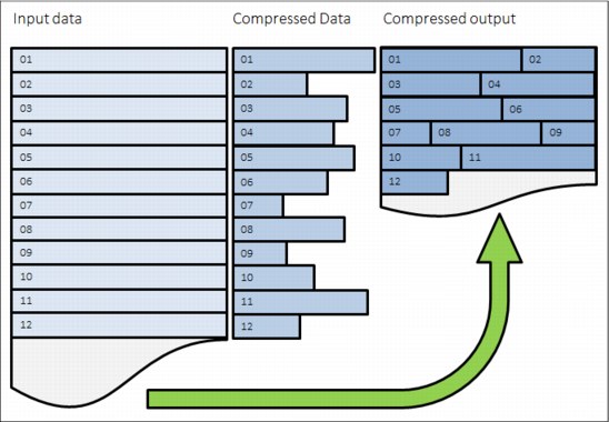
Figure 9-27 Traditional data compression in storage systems
Random Access Compression Engine
The IBM patented RACE implements an inverted approach when compared to traditional approaches to compression. RACE uses variable-size chunks for the input, and produces fixed-size chunks for the output.
This method enables an efficient and consistent way to index the compressed data because it is stored in fixed-size containers (Figure 9-28).

Figure 9-28 Random Access Compression
Location-based compression
Both compression utilities and traditional storage systems compression compress data by finding repetitions of bytes within the chunk that is being compressed. The compression ratio of this chunk depends on how many repetitions can be detected within it. The number of repetitions is affected by how much the bytes stored in the chunk are related to each other. The relation between bytes is driven by the format of the object. For example, an office document might contain textual information and an embedded drawing.
Because the chunking of the file is arbitrary, it has no concept of how the data is laid out within the document. Therefore, a compressed chunk can be a mixture of the textual information and part of the drawing. This process yields a lower compression ratio because the different data types mixed together cause a suboptimal dictionary of repetitions. Which means that fewer repetitions can be detected, because a repetition of bytes in a text object is unlikely to be found in a drawing.
This traditional approach to data compression is also called location-based compression. The data repetition detection is based on the location of data within the same chunk.
Predecide mechanism
Some data chunks have a higher compression ratio than others. Compressing some of the chunks saves little space, but still requires resources, such as processor (CPU) and memory. To avoid spending resources on incompressible data, and to provide the ability to use a different, more effective compression algorithm.
The chunks that are below a given compression ratio are skipped by the compression engine, saving CPU time and memory processing. Chunks that are not compressed with the main compression algorithm, but that still can be compressed well with the other, are marked and processed accordingly. The result might vary because predecide does not check the entire block, only a sample of it.
Figure 9-29 shows how the detection mechanism works.

Figure 9-29 Detection mechanism
Temporal compression
RACE offers a technology leap beyond location-based compression, called temporal compression. When host writes arrive to RACE, they are compressed and fill up fixed size chunks, also named as compressed blocks. Multiple compressed writes can be aggregated into a single compressed block. A dictionary of the detected repetitions is stored within the compressed block.
When applications write new data or update existing data, it is typically sent from the host to the storage system as a series of writes. Because these writes are likely to originate from the same application and be of the same data type, more repetitions are usually detected by the compression algorithm. This type of data compression is called temporal compression because the data repetition detection is based on the time the data was written into the same compressed block.
Temporal compression adds the time dimension that is not available to other compression algorithms. It offers a higher compression ratio because the compressed data in a block represents a more homogeneous set of input data.
Figure 9-30 shows how three writes sent one after the other by a host end up in different chunks. They get compressed in different chunks because their location in the volume is not adjacent. This process yields a lower compression ratio because the same data must be compressed non-natively by using three separate dictionaries.

Figure 9-30 Location-based compression
When the same three writes are sent through RACE, as shown on Figure 9-31, the writes are compressed together by using a single dictionary. This process yields a higher compression ratio than location-based compression (Figure 9-31).

Figure 9-31 Temporal compression
9.4.4 Random Access Compression Engine in IBM Spectrum Virtualize stack
RACE technology is implemented into the Storwize thin provisioning layer and is an organic part of the stack. Compression is transparently integrated with existing system management design. All of the IBM Storwize V5000 Gen2 advanced features are supported on compressed volumes. You can create, delete, migrate, map (assign), and unmap (unassign) a compressed volume as though it were a fully allocated volume.
In addition, you can use Real-time Compression along with Easy Tier on the same volumes. This compression method provides non disruptive conversion between compressed and decompressed volumes. This conversion provides a uniform user-experience and eliminates the need for special procedures when dealing with compressed volumes.
9.4.5 Data write flow
When a host sends a write request to the IBM Storwize V5000 Gen2, it reaches the upper cache layer. The host is immediately sent an acknowledgment of its I/Os.
When the upper cache layer destages to the RACE, the I/Os are sent to the thin-provisioning layer. They are then sent to RACE, and if necessary, to the original host write or writes. The metadata that holds the index of the compressed volume is updated if needed, and is compressed as well.
9.4.6 Data read flow
When a host sends a read request to the IBM Storwize V5000 Gen2 for compressed data, it is forwarded directly to the Real-time Compression component:
•If the Real-time Compression component contains the requested data, IBM Spectrum Virtualize cache replies to the host with the requested data without having to read the data from the lower-level cache or disk.
•If the Real-time Compression component does not contain the requested data, the request is forwarded to the Storwize IBM Spectrum Virtualize lower-level cache.
•If the lower-level cache contains the requested data, it is sent up the stack and returned to the host without accessing the storage.
•If the lower-level cache does not contain the requested data, it sends a read request to the storage for the requested data.
9.4.7 Compression of existing data
In addition to compressing data in real time, you can also compress existing data sets (convert volume to compressed). To do so, you must change the capacity savings settings of the volume:
1. Right-click a particular volume and select Modify Capacity Settings, as shown in Figure 9-32 on page 475.

Figure 9-32 Modifying Capacity Settings

Figure 9-33 Selecting Capacity Setting
3. After the copies are fully synchronized, the original volume copy is deleted automatically. As a result, you have compressed data on the existing volume. This process is non disruptive, so the data remains online and accessible by applications and users.
With virtualization of external storage systems, the ability to compress already stored data significantly enhances and accelerates the benefit to users. It enables them to see a tremendous return on their IBM Storwize V5000 Gen2 investment.
On initial purchase of a IBM Storwize V5000 Gen2 with Real-time Compression, customers can defer their purchase of new storage. As new storage needs to be acquired, IT purchases a lower amount of the required storage before compression.
|
Important: Remember that IBM Storwize V5000 Gen2 will reserve some of its resources like CPU cores and RAM after you create just one compressed volume or volume copy. This setting can affect your system performance if you do not plan accordingly in advance.
|
9.4.8 Configuring compressed volumes
To use compression on the IBM Storwize V5000 Gen2, licensing is required. With the IBM Storwize V5000 Gen2, Real-time Compression is licensed by enclosure. Every enclosure that works with compression needs to be licensed. There are two ways of creating a compressed volume: Basic and Custom.
To create a compressed volume using Basic option, complete the following steps:
1. Navigate to Volumes → Volumes and click Create Volumes.
3. Click Create to finish the compressed volume creation.

Figure 9-34 Creating Basic compressed volume
To create a compressed volume using the Custom option, complete the following steps:
1. Navigate to Volumes → Volumes and click Create Volumes.
2. Select the Custom tab and complete the required information.

Figure 9-35 Creating Advanced compressed volume
If the volume being created through the Custom tab is the first compressed volume in the environment, a warning message displays, as shown in Figure 9-36.
Figure 9-36 First compressed volume warning
9.4.9 Comprestimator
The built-in Comprestimator is a command-line utility that can be used to estimate an expected compression rate for a specific volume. Comprestimator uses advanced mathematical and statistical algorithms to perform the sampling and analysis process in a short and efficient way. The utility also displays its accuracy level by showing the maximum error range of the results achieved based on the formulas that it uses. The following commands are available:
•The analyzevdisk command provides an option to analyze a single volume:
– Usage: analyzevdisk <volume ID>
– Example: analyzevdisk 0
This command can be canceled by running analyzevdisk <volume ID> -cancel.
•The lsvdiskanalysis command provides a list and the status of the volumes. Some of them can be analyzed already, some of them not yet. The command can either be used for all volumes on the system or per volume, similar to lsvdisk (Example 9-11).
Example 9-11 Example of the command run over one volume with ID 0
IBM_2078:ITSO Gen2:superuser>lsvdiskanalysis 0
id 0
name SQL_Data0
state estimated
started_time 151012104343
analysis_time 151012104353
capacity 300.00GB
thin_size 290.85GB
thin_savings 9.15GB
thin_savings_ratio 3.05
compressed_size 141.58GB
compression_savings 149.26GB
compression_savings_ratio 51.32
total_savings 158.42GB
total_savings_ratio 52.80
accuracy 4.97
The state parameter can have the following values:
– idle. Was never estimated and not currently scheduled.
– scheduled. Volume is queued for estimation, and will be processed based on lowest volume ID first.
– active. Volume is being analyzed.
– canceling. Volume was requested to cancel an active analysis, but the analysis was not canceled yet.
– estimated. Volume was analyzed and results show the expected savings of thin provisioning and compression.
– sparse. Volume was analyzed but Comprestimator could not find enough nonzero samples to establish a good estimation.
– compression_savings_ratio. The compression saving ratio is the estimated amount of space that can be saved on the storage in the frame of this specific volume expressed as a percentage.
•The analyzevdiskbysystem command provides an option to run Comprestimator on all volumes within the system. The analyzing process is nondisruptive and should not affect the system significantly. Analysis speed might vary due to the fullness of the volume, but should not take more than a few minutes per volume. This command can be canceled by running the analyzevdiskbysystem -cancel command.
•The lsvdiskanalysisprogress command shows the progress of the Comprestimator analysis, as shown in Example 9-12.
Example 9-12 Comprestimator progress
id vdisk_count pending_analysis estimated_completion_time
0 45 12 151012154400
..................Content has been hidden....................
You can't read the all page of ebook, please click here login for view all page.