CHAPTER 2

PARADATA FOR NONRESPONSE ERROR INVESTIGATION

FRAUKE KREUTER

University of Maryland and IAB/LMU

KRISTEN OLSON

University of Nebraska-Lincoln

2.1 INTRODUCTION

Nonresponse is a ubiquitous feature of almost all surveys, no matter which mode is used for data collection (Dillman et al., 2002) whether the sample units are households or establishments (Willimack et al., 2002) or whether the survey is mandatory or not (Navarro et al., 2012). Nonresponse leads to loss in efficiency and increases in survey costs if a target sample size of respondents is needed. Nonresponse can also lead to bias in the resulting estimates if the mechanism that leads to nonresponse is related to the survey variables (Groves, 2006). Confronted with this fact, survey researchers search for strategies to reduce nonresponse rates and to reduce nonresponse bias or at least to assess the magnitude of any nonresponse bias in the resulting data. Paradata can be used to support all of these tasks, either prior to the data collection to develop best strategies based on past experiences, during data collection using paradata from the ongoing process, or post hoc when empirically examining the risk of nonresponse bias in survey estimates or when developing weights or other forms of nonresponse adjustment. This chapter will start with a description of the different sources of paradata relevant for nonresponse error investigation, followed by a discussion about the use of paradata to improve data collection efficiency, examples of the use of paradata for nonresponse bias assessment and reduction, and some data management issues that arise when working with paradata.

2.2 SOURCES AND NATURE OF PARADATA FOR NONRESPONSE ERROR INVESTIGATION

Paradata available for nonresponse error investigation can come from a variety of different sources, depending on the mode of data collection, the data collection software used, and the standard practice at the data collection agency. Just like paradata for measurement error or other error sources, paradata used for nonresponse error purposes are a by-product of the data collection process or, in the case of interviewer observations, can be collected during the data collection process. A key characteristic that makes a given set of paradata suitable for nonresponse error investigation is their availability for all sample units, respondents and nonrespondents. We will come back to this point in Section 2.3.

Available paradata for nonresponse error investigation vary by mode. For face-to-face and telephone surveys, such paradata can be grouped into three main categories: data reflecting each recruitment attempt (often called “call history” data), interviewer observations, and measures of the interviewer–householder interactions. In principle, such data are available for responding and nonresponding sampling units, although measures of the interviewer–householder interaction and some observations of household members might only be available for contacted persons. For mail and web surveys, call history data are available (where “call” could be the mail invitation to participate in the survey or an email reminder), but paradata collected by interviewers such as interviewer observations and measures of the interviewer–householder interaction are obviously missing for these modes.

2.2.1 Call History Data

Many survey data collection firms keep records of each recruitment attempt to a sampled unit (a case). Such records are now common in both Computer-Assisted Telephone Interviews (CATI) and Computer-Assisted Personal Interviews (CAPI), and similar records can be kept in mail and web surveys. The datasets usually report the date and time a recruitment attempt was made and the outcome of each attempt. Each of these attempts is referred to as a call even if it is done in-person as part of a face-to-face survey or in writing as part of a mail or web survey. Outcomes can include a completed interview, noncontacts, refusals, ineligibility, or outcomes that indicate unknown eligibility. The American Association for Public Opinion Research (AAPOR) has developed a set of mode-specific disposition codes for a wide range of call and case outcomes (AAPOR, 2011). A discussion of adapting disposition codes to the cross-national context can be found in Blom (2008).

A call record dataset has multiple observations for each sampled case, one corresponding to each call attempt. Table 2.1 shows an excerpt of a call record with minimal information kept at each call attempt. Each call attempt to each sampled case, identified with the case ID column, is a row of the dataset. The columns are the date, time, and outcome of each call attempt. For example, case number 10011 had three call attempts (call ID), made on June 1, 2, and 5, 2012 (Date), each at different times of the day. The first call attempt had an outcome code of 3130, which corresponded to a “no answer” outcome (the company follows the AAPOR (2011) standard definitions for outcome codes whenever possible), the second attempt had an outcome of 2111, corresponding to a household-level refusal, and the final call attempt yielded an interview with an outcome code of 1000. Case ID 10012 had two call attempts, one with a telephone answering device (3140) and one that identified that the household had no eligible respondent (4700). Case ID 10013 had only one call attempt in which it was identified as a business (4510). Case ID 10014 had four call attempts, three of which were not answered (3130), and the final that yielded a completed interview (1000). Since each organization may use a different set of call outcome codes, it is critical to have a crosswalk between the outcome code and the actual outcome prior to beginning data collection.

Table 2.1 Example Call Records for Four Cases with IDs 10011–10014

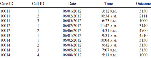
This call record file is different from a final disposition file which (ideally) summarizes the outcome of all calls to a case at the end of the data collection period. Final disposition files have only one row per observation. In some sample management systems, final disposition files are automatically updated using the last outcome from the call record file. In other sample management systems or data collection organizations, final disposition files are maintained separately from the call record and are manually updated as cases are contacted, interviewed, designated as final refusals, ineligibles, and so on. Notably—and a challenge for beginning users of paradata files—final disposition files and call record files often disagree. For instance, a final status may indicate “noncontact,” but the call record files indicate that the case was in fact contacted. Often in this instance, the final disposition file has recorded the outcome of the last call attempt (e.g., a noncontact), but does not summarize the outcome of the case over all of the call attempts made to it. Another challenge for paradata users occurs when the final disposition file indicates that an interview was completed (and there are data in the interview file), but the attempt with the interview does not appear in the call record. This situation often occurs when the final disposition file and the call records are maintained separately. We return to these data management issues in Section 2.6.

How call records are created varies by mode. In face-to-face surveys, interviewers record the date, time, and outcome in a sample management system which may or may not also record when the call record itself was created. In telephone surveys, call scheduling, or sample management systems will often automatically keep track of each call and create a digital record of the calling time; interviewers then supplement the information with the outcome of the call. Mail surveys are not computerized, so any call record paradata must be created and maintained by the research organization. Finally, many web survey software programs record when emails are sent out and when the web survey is completed, but not all will record intermediate outcomes such as undeliverable emails, accessing the web survey without completing it, or clarification emails sent to the survey organization from the respondent.

Figure 2.1 shows a paper and pencil version of a call record form for a face-to-face survey. This form, called a contact form in the European Social Survey (ESS) in 2010, presents the call attempts in sequential order in a table. The table where the interviewer records each individual “visits” to the case is part of a larger contact form that includes the respondent and interviewer IDs. These paper and pencil forms must be data entered at a later time to be used for analysis.

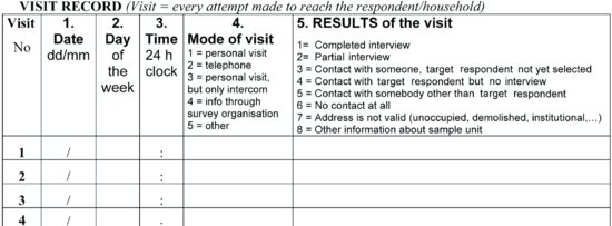
In the case of the ESS, the call record data include call-level characteristics, such as the mode of the attempt (telephone, in-person, etc.). Other surveys might include information on whether an answering machine message was left (in telephone surveys), whether the interviewer left a “sorry I missed you” card (in face-to-face surveys), or whether the case was offered incentives, among other information. For example, U.S. Census Bureau interviewers can choose from a list of 23 such techniques to indicate the strategies they used at each call using the Census Bureau's contact history instrument (CHI; see Figure 2.2).

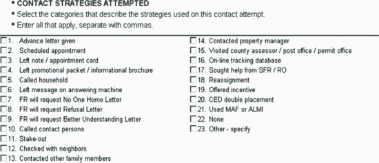
The CHI data are entered on a laptop that the interviewer uses for in-person data collection. Some firms have interviewers collect call record data for face-to-face surveys on paper to make recordings easier when interviewers approach the household. Other firms use a portable handheld computer to collect data at the respondent's doorstep during the recruitment process.1 The handheld device automatically captures time and date of call, and the data are transmitted nightly to the central office. Modern devices allow not only capture of a call's day and time but also latitude and longitude through global positioning software and thus can also be used to monitor or control the work of interviewers and listers (García et al., 2007).

The automatic capturing of date and time information in face-to-face surveys is a big advantage compared to other systems that require the interviewer to enter this information. In particular, at the doorstep, interviewers are busy (and should be) getting the potential respondents to participate in the survey. Also, automatic capturing of call records is consistent with paradata being a true by-product of the data collection process. However, just like paper and pencil entries or entries into laptops, the use of handheld devices can also lead to missed call attempt data if interviewers forget to record a visit when they drive by a house and see that nobody is at home from a distance (Biemer et al., 2013). Chapter 14 continues this discussion of measurement error in call record data.

2.2.2 Interviewer Observations

In addition to call record data, some survey organizations charge interviewers with making observations about the housing unit or the sampled person themselves. This information is most easily collected in face-to-face surveys. Observations of housing units, for example, typically include an assessment of whether the unit is in a multi-unit structure or a building that uses an intercom system. These pieces of information reflect access impediments, for which interviewers might try to use the telephone to contact a respondent prior to the next visit or leave a note at the doorstep. These sorts of observations have been made in several U.S. surveys including the American National Election Studies (ANES), the National Survey of Family Growth (NSFG), the Survey of Consumer Finances (SCF), the Residential Energy Consumption Survey (RECS), and the National Survey of Drug Use and Health (NSDUH), as well as non-U.S. surveys, including the British Crime Survey (BCS), the British Survey of Social Attitudes (BSSA), and the ESS, to name just a few. Observations about items that are related to the questionnaire items themselves can also be useful for nonresponse error evaluation, such as the presence of political signs in the lawn or windows of the housing unit in the ANES or the presence of bars on the windows or burglar alarms in the BCS or the German DEFECT survey (see below). Just like call record data, interviewer observations on housing units can be collected in face-to-face surveys for all sampled units, including noncontacted units.

Potentially more useful for purposes of nonresponse error investigation are observations on individual members of a housing unit. These kinds of observations, typically only available for sample units in which a member of the housing unit has been contacted, may be on demographic characteristics of a household member or on characteristics that are highly correlated with key survey variables. In an ideal case, these interviewer observations have no measurement error, and they capture exactly what the respondent would have reported about those same characteristics (if these were also reported without error). Observations of demographic characteristics, such as age (Matsuo et al., 2010; Sinibaldi, 2010), sex (Matsuo et al., 2010), race (Smith, 1997; Burns et al., 2001; Smith, 2001; Lynn, 2003; Saperstein, 2006), income (Kennickell, 2000; Burns et al., 2001), and the presence of non-English speakers (Bates et al., 2008; National Center for Health Statistics, 2009) are made in the ESS, the General Social Survey in the United States, the U.S. SCF, the BCS, and the National Health Interview Survey. Although most of these observations require in-person interviewers for collection, gender has been collected in CATI surveys based on vocal characteristics of the household informant, although this observation has not been systematically collected and analyzed for both respondents and nonrespondents (McCulloch, 2012).

Some surveys like the ESS, the Los Angeles Family and Neighborhood Study (LAFANS), the SCF, the NSFG, the BCS, and the Health and Retirement Study (HRS) ask interviewers to make observations about the sampled neighborhood. The level of detail with which these data are collected varies greatly across these surveys. Often, the interviewer is asked to make several observations about the state of the neighborhood surrounding the selected household and to record the presence or absence of certain housing unit (or household) features. These data can be collected once—at the first visit to a sampled unit in the neighborhood, for example—or collected multiple times over the course of a long data collection period.

The observation of certain features can pose a challenge to the interviewers, and measurement errors are not uncommon. Interviewer observations can be collected relatively easily in face-to-face surveys, but they are virtually impossible to obtain (without incurring huge costs) in mail or web surveys. Innovative data collection approaches such as Nielsen's Life360 project integrate surveys with smartphones, asking respondents to document their surroundings by taking a photograph while also completing a survey on a mobile device (Lai et al., 2010). Earlier efforts to capture visual images for the neighborhoods of all sample units were made in the DEFECT study (Schnell and Kreuter, 2000), where photographs of all street segments were taken during the housing unit listing process, and in the Project on Human Development in Chicago Neighborhoods, where trained observers took videos from all neighborhoods in which the survey was conducted (Earls et al., 1997; Raudenbush and Sampson, 1999). Although not paradata per se, similar images from online sources such as Google Earth could provide rich data about neighborhoods of sampled housing units in modes other than face-to-face surveys. Additionally, travel surveys are increasingly moving away from diaries and moving toward using global positioning devices to capture travel behaviors (Wolf et al., 2001; Asakura and Hato, 2009).

2.2.3 Measures of the Interviewer–Householder Interaction

A key element in convincing sample units to participate in the survey is the actual interaction between the interviewer and household members. Face-to-face interviewers' success depends in part on the impression they make on the sample unit. Likewise telephone interviewers' success is due, at least in part, to what they communicate about themselves. This necessarily includes the sound of their voices, the manner and content of their speech, and how they interact with potential respondents. If the interaction between an interviewer and householder is recorded, each of these properties can be turned into measurements and paradata for analysis purposes. For example, characteristics of interactions such as telephone interviewers' speech rate and pitch, measured through acoustic analyses of audio-recorded interviewer introductions, have been shown to be associated with survey response rates (Sharf and Lehman, 1984; Oksenberg and Cannell, 1988; Groves et al., 2008; Benki et al., 2011; Conrad et al., 2013).

Long before actual recordings of these interactions were first analyzed for acoustic properties (either on the phone or through the CAPI computer in face-to-face surveys), survey researchers were interested in capturing other parts of the doorstep interaction (Morton-Williams, 1993; Groves and Couper, 1998). In particular, they were interested in the actual reasons sampled units give for nonparticipation. In many cases, interviewers record such reasons in the call records (also called contact protocol forms, interviewer observations, or contact observations), although audio recordings have been used to identify the content of this interaction (Morton-Williams, 1993; Campanelli et al., 1997; Couper and Groves, 2002). Many survey organizations also use contact observations to be informed about the interaction so that they can prepare a returning interviewer for the next visit or send persuasion letters. Several surveys conducted by the U.S. Census Bureau require interviewers to capture some of the doorstep statements in the CHI. An alternative type of contact observation is the interviewer's subjective assessment of the householder's reluctance or willingness to participate on future contacts. NSFG, for example, collects an interviewer's estimates of the likelihood of an active household participating after 7 weeks of data collection in a given quarter (Lepkowski et al., 2010). While these indicators are often summarized under the label “doorstep interactions”, they can be captured just as easily on a telephone survey (Eckman et al., forthcoming).

Any of these doorstep interactions may be recorded on the first contact with the sampled household or on every contact with the household. The resulting data structure can pose unique challenges when modeling paradata.

We have examined where paradata on respondents and nonrespondents can be collected and how this varies by mode. The exact nature of those data and a decision on what variables should be formed out of those data depends on the purpose of analysis, on the hypotheses one has in a given context about the nonresponse mechanism, and on the survey content itself. Unfortunately, it is often easier to study nonresponse using paradata in interviewer-administered—and especially in-person—surveys than in self-administered surveys. The next section will give some background to help guide the decisions about what to collect for what purpose.

2.3 NONRESPONSE RATES AND NONRESPONSE BIAS

There are two aspects of nonresponse bias about which survey practitioners worry—nonresponse rates and the difference between respondents and nonrespondents on a survey statistic of interest. In its most simple form, the nonresponse rate is the ratio of missing respondents (M) divided by the total number of cases in the sample (N), assuming for simplicity that all sampled cases are eligible to respond to the survey. A high nonresponse rate means a reduction in the number of actual survey responses and thus poses a threat to the precision of statistical estimates—standard errors and respectively confidence intervals get smaller with increased sample size. A survey with a high nonresponse rate can however still lead to an unbiased estimate if there is no difference between respondents and nonrespondents on a survey statistic of interest, or said another way, if the process that leads to participation in the survey is unrelated to the survey statistic of interest.

The two equations for nonresponse bias of an unadjusted respondent mean presented below clarify this:

(2.1)

If the difference between the average value for respondents on a survey variable (R) is identical to the average value of all missing cases on that same variable (M) then the second term in the estimation of the bias (Bias(R)) in Equation 2.1 is zero. Thus, even if the nonresponse rate (M/N) is high there will not be any nonresponse bias for this survey statistic. Unfortunately, knowing the difference between respondents and nonrespondents on a survey variable of interest is often impossible. After all, if the values of Y are known for both respondents and nonrespondents, there is no need to conduct a survey. Some paradata we discuss in this chapter carry the hope that they are good proxy variables for key survey statistics and can provide an estimate for the difference between R and M. We also note that a nonresponse bias assessment is always done with respect to a particular outcome variable. It is likely that a survey shows nonresponse bias on one variable, but not on another (Groves and Peytcheva, 2008).

Another useful nonresponse bias equation is given by Bethlehem (2002) and is often referred to as the stochastic model of nonresponse bias. Here, sampled units explicitly have a nonzero probability of participating in the survey, also called response propensity, represented by ρ.

(2.2)

The covariance term between the survey variable and the response propensity σyρ will be greater than zero if the survey variable itself is the reason someone participates in the survey.2 This situation is often referred to as nonignorable nonresponse or a unit not missing at random (Little and Rubin, 2002). The covariance is also positive when a third variable jointly affects the participation decision and the outcome variables. This situation is sometimes called ignorable nonresponse or a unit missing at random. Knowing which variables might affect both the participation decision and the outcome variables is therefore crucial to understanding the nonresponse bias of survey statistics. In many surveys, no variables are observed for nonrespondents, and therefore it is difficult to empirically measure any relationship between potential third variables and the participation decision (let alone the unobserved survey variables for nonrespondents).

A sampled unit's response propensity cannot be directly observed. We can only estimate the propensity from information that we obtained on both respondents and nonrespondents. Traditional weighting methods for nonresponse adjustment obtain estimates of response rates for particular subgroups; these subgroup response rates are estimates of response propensities in which all members of that subgroup have the same response propensity. When multiple variables are available on both respondents and nonrespondents, a common method for estimating response propensities uses a logistic regression model to predict the dichotomous outcome of survey participation versus nonparticipation as a function of these auxiliary variables. Predicted probabilities for each sampled unit estimated from this model constitute estimates of response propensities. Chapter 12 will show examples of such a model.

Paradata can play an important role in these analyses examining nonresponse bias and in predicting survey participation. Paradata can be observed for both respondents and nonrespondents, thus meeting the first criterion of being available for analyses. Their relationship to survey variables of interest can be examined for responding cases, thus providing an empirical estimate of the covariance term in Equation 2.2. Useful paradata will likely differ across surveys because the participation decision is sometimes dependent on the survey topic or sponsor (Groves et al., 2000), and proxy measures of key survey variables will thus naturally vary across surveys and survey topics (Kreuter et al., 2010b). Within the same survey, some paradata will be strong predictors of survey participation but vary in their association with the important survey variables (Kreuter and Olson, 2011). The guidance from the statistical formulas suggest that theoretical support is needed to determine which paradata could be proxy measures of those jointly influential variables or what may predict survey participation.

Three things should be remembered from this section: (1) the nonresponse rate does not directly inform us about the nonresponse bias of a given survey statistic, (2) if paradata are proxy variables of the survey outcome, they can provide estimates of the difference between nonrespondents and respondents on that survey variable, and when this information is combined with the nonresponse rate, then an estimate of nonresponse bias for that survey statistic can be obtained; and (3) to estimate response propensities, information on both respondents and nonrespondents are needed; paradata can be available for both respondents and nonrespondents.

2.3.1 Studying Nonresponse with Paradata

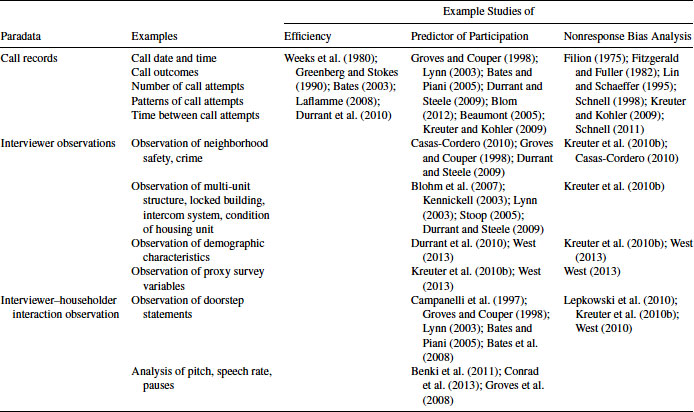
Studies of nonresponse using paradata have focused on three main areas: (1) methods to improve the efficiency of data collection, (2) predictors of survey participation, contact, and cooperation, and (3) assessment of nonresponse bias in survey estimates. These examinations may be done concurrently with data collection or in a post hoc analysis. The types of paradata used for each type of investigation vary, with interviewer observations (in combination with frame and other auxiliary data) used more frequently for predictors of survey participation, call record data used to examine efficiency, and nonresponse bias diagnoses using both observational data and call record data. Table 2.2 summarizes these uses of each type of paradata and identifies a few exemplar studies of how these paradata have been used for purposes of efficiency, as a predictor of survey participation, contact or cooperation, or for nonresponse bias analyses.

Table 2.2 Type of Paradata Used by Purpose

2.3.2 Call Records

Data from call records have received the most empirical attention as a potential source of identifying methods to increase efficiency of data collection and to explain survey participation, with somewhat more limited attention paid to issues related to nonresponse bias. Call records are used both concurrently and for post hoc analyses. One of the primary uses of call record data for efficiency purposes is to determine and optimize call schedules in CATI, and occasionally CAPI, surveys. Generally, post hoc analyses have revealed that call attempts made during weekday evenings and weekends yield higher contact rates than calls made during weekdays (Weeks et al., 1980, 1987; Hoagland et al., 1988; Greenberg and Stokes, 1990; Groves and Couper, 1998; Odom and Kalsbeek, 1999; Bates, 2003; Laflamme, 2008; Durrant et al., 2010), and that a “cooling off” period between an initial refusal and a refusal conversion effort can be helpful for increasing participation (Tripplett et al., 2001; Beullens et al., 2010). On the other hand, calling to identify ineligible cases such as businesses and nonworking numbers is more efficiently conducted during the day on weekdays (Hansen, 2008).

Results from these post hoc analyses can be programmed into a CATI call scheduler to identify the days and times at which to allocate certain cases to interviewers. For most survey organizations, the main purpose of keeping call record data is to monitor response rates, to know which cases have not received a minimum number of contact attempts, and to remove consistent refusals from the calling or mailing/emailing queue. Call records accumulated during data collection can be analyzed and used concurrently with data collection itself. In fact, most CATI software systems have a “call window” or “time slice” feature to help the researcher ensure that sampled cases are called during different time periods and different days of the week, drawing on previous call attempts as recorded in the call records. In some surveys, interviewers are encouraged to mimic such behavior and asked to vary the times at which they call on sampled units. Contact data that the interviewer keeps can help guide her efforts. Web and mail surveys are less sensitive to the day and time issue, but call records are still useful as an indicator of when prior recruitment attempts are no longer effective.

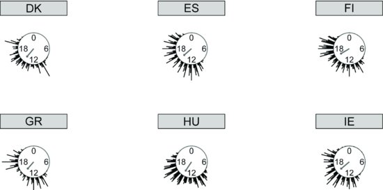
“Best times to call” are population dependent, and in cross-national surveys, country-specific “cultures” need to be taken into account (see Stoop et al., 2010 for the ESS). When data from face-to-face surveys are used to model “optimal call windows,” one also needs to be aware that post hoc observational data include interviewer-specific preferences (Purdon et al., 1999). That is, unlike in CATI surveys sampled cases in face-to-face surveys are not randomly assigned to call windows (see Chapters 12 and 7 for a discussion of this problem). Figure 2.3 shows frequencies of calls by time of day for selected countries in the ESS. Each circle represents a 24-h clock, and the lines coming off of the circle represent the relative frequency of calls made at that time. Longer lines are times at which calls are more likely to be made. This figure shows that afternoons are much less popular calling times in Greece (GR) than in Hungary (HU) or Spain (ES).

Examining the relationship between field effort and survey participation is one of the most common uses of call history data. Longer field periods yield higher response rates as the number of contact attempts increases and timing of call attempts becomes increasingly varied (Groves and Couper, 1998), but the effectiveness of repeated similar recruitment attempts diminishes over time (Olson and Groves, 2012). This information can be examined concurrently with data collection itself. It is common for survey organizations to monitor the daily and cumulative response rate over the course of data collection using information obtained from the call records. Survey organizations often also use call records after the data are collected to examine several “what if” scenarios, to see, for example, how response rates or costs would have changed had fewer calls been made (Kalsbeek et al., 1994; Curtin et al., 2000; Montaquila et al., 2008).

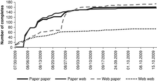
Daily monitoring can be done in both interviewer-administered and self-administered surveys. Figure 2.4 shows an example from the Quality of Life in a Changing Nebraska Survey, a web and mail survey of Nebraska residents. The x-axis shows the date in the field period and the y-axis shows the cumulative number of completed questionnaires. Each line corresponds to a different experimental mode condition. The graph clearly shows that the conditions with a web component yielded earlier returns than the mail surveys, as expected, but the mail surveys quickly outpaced the web surveys in the number of completes. The effect of the reminder mailing (sent out on August 19) is also clearly visible, especially in the condition that switched from a web mode to a mail mode at this time.

In general, post hoc analyses show that sampled units who require more call attempts are more difficult to contact or more reluctant to participate (Campanelli et al., 1997; Groves and Couper, 1998; Lin et al., 1999; Olson, 2006; Blom, 2012). Although most models of survey participation use logistic or probit models to predict survey participation, direct use of the number of call attempts in these post hoc models has given rise to endogeneity concerns. The primary issue is that the number of contact attempts is, in many instances, determined by whether the case has been contacted or interviewed during the field period. After all, interviewed cases receive no more follow-up attempts. Different modeling forms have been used as a result. The most commonly used model is a discrete time hazard model, in which the outcome is the conditional probability of an interview on a given call, given no contact or participation on prior calls (Kennickell, 1999; Groves and Heeringa, 2006; Durrant and Steele, 2009; West and Groves, 2011; Olson and Groves, 2012). See Chapter 12 by Durrant and colleagues for a thorough discussion and example of these models. Active use of propensity models concurrent with data collection is discussed in Chapter 7 by Wagner and Chapter 6 by Kirgis and Lepkowski in the context of responsive designs.

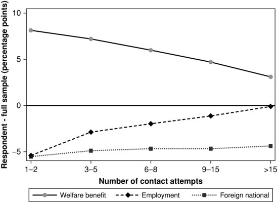
Call record data can also be used for nonresponse bias analyses, although these analyses are most often done after data collection finishes. In such investigations, the number of call attempts to obtain a completed interview is hypothesized to be (linearly) related to both response propensity (a negative relationship) and to important survey characteristics (either positively or negatively), that is, there is a “continuum of resistance” (Filion, 1975; Fitzgerald and Fuller, 1982; Lin and Schaeffer, 1995; Bates and Creighton, 2000; Lahaut et al., 2003; Olson, 2013). Alternatively, these analyses have been used to be diagnostic of whether there is a covariance between the number of contact attempts and important survey variables, with the goal to have insight into the covariance term in the numerator of Equation 2.2. Figure 2.5 shows one example of using call record data to diagnose nonresponse bias over the course of data collection (Kreuter et al., 2010a). These data come from the Panel Study of Labor Market and Social Security (PASS) conducted at the German Institute for Employment Research (Trappmann et al., 2010). In this particular example nonresponse bias could be assessed using call record data and administrative data available for both respondents and nonrespondents. The three estimates of interest are the proportion of persons who received a particular type of unemployment benefit, whether or not the individual was employed, and whether or not the individual was not a German citizen. The x-axis represents the total number of call attempts made to a sampled person, from 1–2 call attempts to more than 15 call attempts. The y-axis represents the percent relative difference between the estimate calculated as each call attempt group is cumulated into the estimate and the full sample estimate. For example, the three to five call attempts group includes both those who were contacted after one or two call attempts and those who were contacted with three to five attempts. If the line approaches zero, then nonresponse bias of the survey estimate is reduced with additional contact attempts. For welfare benefits and employment status we can see that this is the case and nonresponse bias is reduced, although the magnitude of the reduction varies over the two statistics. For the indicator of being a foreign citizen, there is little reduction in nonresponse bias of the estimate with additional contact attempts.

An alternative version of this approach are models in which the number of call attempts and call outcomes are used to categorize respondents and nonrespondents into groups of “easy” and “difficult” cases (Lin and Schaeffer, 1995; Laflamme and Jean. Some models disaggregate effort exerted to the case into the patterns of outcomes to different cases such as the proportion of noncontacts out of all calls made, rather than simply number of call attempts (Kreuter and Kohler, 2009).

Montaquila et al. (2008) simulate the effect of various scenarios that limit the use of refusal conversion procedures and the number of call attempts on survey response rates and estimates in two surveys. In these simulations, responding cases who required these extra efforts (e.g., refusal conversion and more than eight screener call attempts) are simulated to be “nonrespondents,” and excluded from calculation of the survey estimates (as in the “what if” scenario described above). Although these simulations show dramatic results on the response rates, the survey estimates show very small differences from the full sample estimate, with the median absolute relative difference under six scenarios never more than 2.4% different from the full sample estimate.

2.3.3 Interviewer Observations

Data resulting from interviewer observations of neighborhoods and sampled housing units has been used primarily for post hoc analyses of correlates of survey participation. For example, interviewer observations of neighborhoods have been used in post hoc analyses to examine the role of social disorganization in survey participation. Social disorganization is an umbrella term that includes a variety of other concepts, among them sometimes population density and crime themselves (Casas-Cordero, 2010), that may affect helping behavior and increase distrust (Wilson, 1985; Franck, 1980). Faced with a survey request, the reduction in helping behavior or the perception of potential harm may translate into refusal (Groves and Couper, 1998). Interviewer observations about an area's safety have been found to be significantly associated with both contactability and cooperation in the United Kingdom (Durrant and Steele, 2009) and in the United States (Lepkowski et al., 2010). Interviewer observations of characteristics of housing units have been used to identify access impediments as predictors of both contact and cooperation in in-person surveys. Observations of whether the sampled unit is in a multi-unit structure versus a single family home, is in a locked building, or has other access impediments have been shown to predict a household's contactability (Campanelli et al., 1997; Groves and Couper, 1998; Kennickell, 2003; Lynn, 2003; Stoop, 2005; Blohm et al., 2007; Sinibaldi, 2008; Maitland et al., 2009; Lepkowski et al., 2010), and the condition of the housing unit relative to others in the area predict both contact and cooperation (Lynn, 2003; Sinibaldi, 2008; Durrant and Steele, 2009). Neighborhood and housing unit characteristics can be easily incorporated into field monitoring in combination with information from call records. For example, variation in response, contact, and cooperation rates for housing units with access impediments versus those without access impediments could be monitored, with a field management goal of minimizing the difference in response rates between these two groups. This kind of monitoring by subgroups is not limited to paradata and can be done very effectively for all data available on a sampling frame. However, in the absence of (useful) frame information, paradata can be very valuable if collected electronically and processed with the call record data.

Observations about demographic characteristics of sampled members can be predictive of survey participation (Groves and Couper, 1998; Stoop, 2005; West, 2013) and can be used to evaluate potential nonresponse bias if they are related to key survey variables of interest. However, to our knowledge, the majority of the work on demographic characteristics and survey participation come from surveys in which this information is available on the frame (Tambor et al., 1993; Lin et al., 1999), from a previous survey (Peytchev et al., 2006), from administrative sources (Schouten et al., 2009), or from looking at variation within the respondent pool (Safir and Tan, 2009) rather than from interviewer observations. Exceptions in which interviewers observe gender and age of the contacted householder include the ESS and the UK Census Link Study (Kreuter et al., 2007; Matsuo et al., 2010; Durrant et al., 2010; West, 2013). As with housing unit or area observations, information about demographic characteristics of sampled persons could be used in monitoring cooperation rates during the field period; since these observations require contact with the household, monitoring variation in contact rates or overall response rates is not possible with this type of interviewer observation.

Observations about proxy measures of important survey variables are, with a few exceptions, a relatively new addition to the set of paradata available for study. Examples of these observations that have been implemented in field data collections include whether or not an alarm system is installed at the house in a survey on fear of crime (Schnell and Kreuter, 2000; Eifler et al., 2009). Some observations are more “guesses” than observations themselves, for example, whether the sampled person is in an active sexual relationship in a fertility survey (Groves et al., 2007; West, 2013), the relative income level of the housing unit for a financial survey (Goodman, 1947), or whether the sampled person is on welfare benefits in a survey on labor market participation (West et al., 2012). Depending on the survey topic one can imagine very different types of observations. For example, in health surveys, the observation of smoking status, body mass, or health limitations may be fruitful for diagnosing nonresponse bias (Maitland et al., 2009; Sinibaldi, 2010). The U.S. Census Bureau is currently exploring indicators along those lines. Other large scale surveys such as PIAAC-Germany experiment with interviewer observations of householders' educational status, which is in the context of PIAAC a proxy variable of a key survey variable.

These types of observations that proxy for survey variables are not yet routinely collected in contemporary surveys, and have only rarely be collected in the survey context for respondents and nonrespondents. As such, recent examinations of these measures focus on post hoc analyses to assess their usefulness in predicting survey participation and important survey variables. These post hoc analyses have shown that although these observational data are not identical to the reports collected from the respondent themselves, they are significantly associated with survey participation and predict important survey variables (West, 2013).

2.3.4 Observations of Interviewer–Householder Interactions

What householders say “on the doorstep” to an interviewer is highly associated with survey cooperation rates (Campanelli et al., 1997; Couper, 1997; Groves and Couper, 1998; Peytchev and Olson, 2007; Bates et al., 2008; Taylor, 2008; Groves et al., 2009; Safir and Tan, 2009). In post hoc analyses of survey participation, studies have shown that householders who make statements such as “I'm not interested” or “I'm too busy” have lower cooperation rates, whereas householders who ask questions have no different or higher cooperation rates than persons who do not make these statements (Morton-Williams, 1993; Campanelli et al., 1997; Couper and Groves, 2002; Olson et al., 2006; Maitland et al., 2009; Dahlhamer and Simile, 2009). As with observations of demographic or proxy survey characteristics, observations of the interviewer–householder interaction require contact with the household and thus can only be used to predict cooperation rates.

These statements can be used concurrently during data collection to tailor follow-up recruitment attempts, such as sending persuasion letters for refusal conversion (Olson et al., 2011) or in tailored refusal aversion efforts (Groves and McGonagle, 2001; Schnell and Trappmann, 2007). Most of these uses happen during data collection and are often undocumented. As such, little is known about what makes certain tailoring strategies more successful or whether one can derive algorithms to predict when given strategies should be implemented.

Contact observations can also be related to the topic of the survey and thus diagnostic of nonresponse bias, such as refusal due to health-related reasons in a health study (Dahlhamer and Simile, 2009) or refusal due to lack of interest in politics in an election study (Peytchev and Olson, 2007). For example, Maitland et al. (2009) found that statements made to the interviewer on the doorstep about not wanting to participate because of health-related reasons were more strongly associated with important survey variables in the National Health Interview Survey than any other contact observation. This finding suggests that recording statements that are survey topic related could be used for diagnosing nonresponse bias, not just as a correlate of survey cooperation.

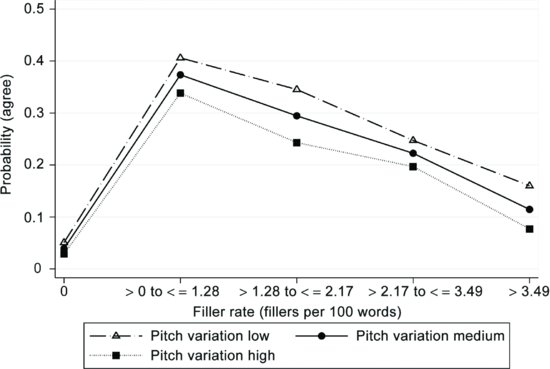
Acoustic measurements of the speech of survey interviewers during recruitment have received recent attention as predictors of survey participation. Although older studies show positive associations between interviewer-level response rates and acoustic vocal properties (Oksenberg and Cannell, 1988), more recent studies show mixed associations between interviewer-level response rates and acoustic measurements (van der Vaart et al., 2006; Groves et al., 2008). One reason for these disparate findings may be related to nonlinearities in the relationship between acoustic measurements and survey outcomes. For example, Conrad et al. (2013) showed a curvilinear relationship between agreement to participate and the level of disfluency in the interviewers' speech across several phone surveys. Using data from Conrad et al. (2013), Figure 2.6 shows that agreement rates (plotted on the y-axis) are lowest when the interviewers spoke without any fillers (e.g.,“uhm” and “ahms”, plotted on the x-axis), often called robotic speech, and highest with a moderate number of fillers per 100 words. An interviewer's pitch also affects agreement rates—here interviewers with low pitch variation in their voice (the dashed line) were on average more successful in recruiting respondents than those with high pitch variation (the dotted line).

To our knowledge, no study to date has looked at the association between these vocal characteristics and nonresponse bias or as a means to systematically improve efficiency of data collection.

2.4 PARADATA AND RESPONSIVE DESIGNS

Responsive designs use paradata to increase the efficiency of survey data collections, estimate response propensities, and evaluate nonresponse bias of survey estimates. As such, all of the types of paradata described above can be—and have been—used as inputs into responsive designs. As described by Groves and Heeringa (2006), responsive designs can use paradata to define “phases” of data collection in which different recruitment protocols are used to monitor “phase capacity” in which the continuation of a current recruitment protocol no longer yields meaningful changes in survey estimates and estimate response propensities from models using paradata to target efforts during the field period. The goal of these efforts is to be responsive to anticipated uncertainties and to adjust the process based on replicable statistical models. In this effort, paradata are used to create progress indicators that can be monitored in real time (see Chapter 9 in this volume for monitoring examples). Chapters 6, 7, and 10 in this volume describe different aspects of the role that paradata plays in responsive designs.

2.5 PARADATA AND NONRESPONSE ADJUSTMENT

Nonresponse bias of a sample estimate occurs when the variables that affect survey participation also are associated with the important survey outcome variables. Thus, effective nonresponse adjustment variables predict both the probability of participating in a survey and the survey variables themselves (Little, 1986; Bethlehem, 2002; Kalton and Flores-Cervantes, 2003; Little and Vartivarian, 2003, 2005; Groves, 2006). For sample-based nonresponse adjustments such as weighting class adjustments or response propensity adjustments, these adjustment variables must be available for both respondents and nonrespondents (Kalton, 1983). The paradata discussed above fit the data availability criterion and generally fit the predictive of survey participation criterion. Where they fall short—or where empirical evidence is lacking—is in predicting important survey variables of interest (Olson, 2013).

How to incorporate paradata into unit nonresponse adjustments is either straightforward or very complicated. One straightforward method involves response propensity models, usually logistic regression models, in which the response indicator is the dependent variable and variables that are expected to predict survey participation, including paradata, are the predictors. The predicted response propensities from these models are then used to create weights (Kalton and Flores-Cervantes, 2003). If the functional form is less clear, or the set of potential predictors prohibitively large, classification models like CHAID or CART might be more suitable. Weights are created from the inverse of the response rates of each group identified in the classification model, consistent with creating weights when paradata are not available.

Alternatively, paradata can be used in “callback models” of various functional forms, but often using explicit probability or latent class models to describe changes in survey estimates across increased levels of effort (Drew and Fuller, 1980; Alho, 1990; Colombo, 1992; Potthoff et al., 1993; Anido and Valdes, 2000; Wood et al., 2006; Biemer and Link, 2006; Biemer and Wang, 2007; Biemer, 2009). These models can be complicated for many data users, requiring knowledge of probability distributions and perhaps requiring specialty software packages such as MPlus or packages that support Bayesian analyses. Another limitation of these more complicated models is that they do not always yield adjustments that can be easily transported from univariate statistics such as means and proportions to multivariate statistics such as correlations or regression coefficients.

In sum, postsurvey adjustment for nonresponse with paradata views paradata in one of the two ways. First, paradata may be an additional input into a set of methods such as weighting class adjustments or response propensity models that a survey organization already employs. Alternatively, paradata may pose an opportunity to develop new methodologies for postsurvey adjustment. Olson (2013) describes a variety of these uses of paradata in postsurvey adjustment models. As paradata collection becomes routine, survey researchers and statisticians should actively evaluate the use of these paradata in both traditional and newly developed adjustment methods.

2.6 ISSUES IN PRACTICE

Although applications of paradata in the nonresponse error context are seemingly straightforward, many practical problems may be encountered when working with paradata, especially call record data. Researchers not used to these data typically struggle with the format, structure and logic of the dataset. The following issues often arise during a first attempt to analyze such data.

Long and Wide Format

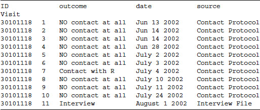
Call record data are available for each contact attempt to each sample unit. This means that there are unequal numbers of observations available for each sample unit. Usually call record data are provided in “long” format, where each row in the dataset is one call attempt, and the attempts made to one sample unit span over several rows (see Table 2.1 and Figure 2.7). In Figure 2.7, ID 30101118 received 11 call attempts, each represented by a row of the dataset. For most analyses this format is quite useful, and we recommend using it. If data are provided in wide format (where each call attempt and the outcome is written in one single row) a transformation to long format is advisable (Kohler and Kreuter (2012), Chapter 11).

Outcome Codes

Figure 2.3 also shows a typical data problem when working with call record data. The case displayed in Figure 2.3 had 10 recorded contact attempts, and was merged with the interview data. Comparing time and date of the contact attempts with time and date the interview was made, one can see that the interview occurred after the last visit in the call record file—that is, the actual interview was not recorded in the call records and there were actually 11 call attempts made to this case. Likewise, final outcome codes assigned by the field work organization often do not match the last outcome recorded in the call record data (e.g., if a refusal case shows several contact attempts with no contacts after the initial refusal, they often are assigned to be a final noncontact rather than a final refusal, see also Blom et al. (2010)). These final outcomes may be recorded in a separate case-level dataset (with one observation per case) or as a final “call attempt” in a call record file, in which the case is “coded out” of the data collection queue. Furthermore, outcome codes are often collected at a level of detail that surpasses the response, (first) contact and cooperation indicators that are needed for most nonresponse analyses (see the outcome codes in Table 2.1). Analysts must make decisions about how to collapse these details for their purposes (see Abraham et al., 2006, for discussion of how different decisions about collapsing outcome codes affect nonresponse analyses).

Structure

Call record data and interviewer observations are usually hierarchical data. That is, the unit of analysis (individual calls) is nested within a higher level unit (sample cases). Likewise, cases are nested within interviewers and, often, within primary sampling units. In face-to-face surveys, such data can have a fully nested structure if cases are assigned to a unique interviewer. In CATI surveys, sample units are usually called by several interviewers. Depending on the research goal, analysis of call record data therefore needs to either treat interviewers as time varying covariates or make a decision as to which interviewer is seen as responsible for a case outcome (for examples of these decisions see West and Olson, 2010). Furthermore, this nesting leads to a lack of independence of observations across calls within sampled units and across sampled units within interviewers. Analysts may choose to aggregate across call attempts for the same individual or to use modeling forms such as discrete time hazard models or multilevel models to adjust for this lack of independence. See Chapter 12 by Durrant and colleagues for a detailed discussion of these statistical models.

Time and Date Information

Processing the rich information on time and dates of call attempts can be quite tedious if data are not available in the right format. Creating an indicator for the time since the last contact attempt requires counting the number of days, and hours (or minutes) that have passed. Fortunately, many software packages have the so-called time and date functions (Kohler and Kreuter (2012), Chapter 5). They typically convert any dates into the number of days passed since, for example, January 1, 1960. Once two dates are converted this way, variables can simply be subtracted from each other to calculate the number of days.

These data management issues frequently occur when analyzing paradata for nonresponse error. Other analytic issues that can arise include how to treat cases with unknown eligibility and how to handle missing data in interviewer observations, both topics that require further empirical investigation.

2.7 SUMMARY AND TAKE HOME MESSAGES

In this chapter, we have examined three types of paradata that can be used to evaluate nonresponse in sample surveys—call history data, interviewer observations of the sampled unit, and measures of the interviewer–householder interaction. These paradata can be collected in surveys of any mode, but are most frequently and fruitfully collected in interviewer-administered surveys. Post hoc analyses of these types of paradata are most often conducted, but they are increasingly being used concurrently with data collection itself for purposes of monitoring and tracking field progress and—potentially—nonresponse error indicators.

When deciding on the collection or formation of paradata for nonresponse error investigation, it is important to be aware of the purpose for which those data will be used. If an increase in efficiency is the goal, different paradata might be useful or necessary than in the investigation of nonresponse bias.

The design of new types of paradata and empirical investigation of existing paradata in new ways are the next steps in this area of paradata for survey researchers and practitioners. Particularly promising is the development of new forms of paradata that proxy for important survey variables. With the collection of new types of data should also come investigations into the quality of these data, and the conditions and analyses for which they are useful.

It is also important to emphasize that survey practitioners and field managers have long been users of certain types of paradata—primarily those from call records—but other forms of paradata have been less systematically used during data collection. Although more organizations are implementing responsive designs and developing “paradata dashboards' (Sirkis, 2012; Craig and Hogue, 2012; Reifschneider and Harris, 2012), use of paradata for design and management of surveys remains far from commonplace. We recommend that survey organizations that do not currently routinely collect and/or analyze paradata start with simpler pieces—daily analysis of call outcomes in call records by subgroups defined by frame information or analysis of productive times and days to call a particular population of interest—and then branch into more extensive development of paradata that requires additional data collection such as interviewer observations. It is only through regular analysis and examination of these paradata that their usefulness for field management becomes apparent.

REFERENCES

AAPOR (2011). Standard Definitions: Final Dispositions of Case Codes and Outcome Rates for Surveys. 7th edition. The American Association for Public Opinion Research.

Abraham, K., Maitland, A., and Bianchi, S. (2006). Nonresponse in the American Time Use Survey: Who is Missing from the Data an How Much Does it Matter? Public Opinion Quarterly, 70(5):676–703.

Alho, J.M. (1990). Adjusting for Nonresponse Bias Using Logistic Regression. Biometrika, 77(3):617–624.

Anido, C. and Valdes, T. (2000). An Iterative Estimating Procedure for Probit-type Nonresponse Models in Surveys with Call Backs. Sociedad de Estadistica e Investigacion Operativa, 9(1):233–253.

Asakura, Y. and Hato, E. (2009). Tracking Individual Travel Behaviour Using Mobile Phones: Recent Technological Development. In Kitamura R., Yoshii T., and Yamamoto T., editors, The Expanding Sphere of Travel Behaviour Research. Selected Papers from the 11th International Conference on Travel Behaviour Research. International Association for Travel Behaviour Research, page 207--233. Emerald Group, Bingley, UK.

Bates, N. (2003). Contact Histories in Personal Visit Surveys: The Survey of Income and Program Participation (SIPP) Methods Panel. Proceedings of the Section on Survey Research Methods, American Statistical Association, pages 7--14.

Bates, N. and Creighton, K. (2000). The Last Five Percent: What Can We Learn from Difficult/Late Interviews? Proceedings of the Section on Government Statistics and Section on Social Statistics, American Statistical Association, pages 120--125.

Bates, N., Dahlhamer, J., and Singer, E. (2008). Privacy Concerns, Too Busy, or Just Not Interested: Using Doorstep Concerns to Predict Survey Nonresponse. Journal of Official Statistics, 24(4):591–612.

Bates, N. and Piani, A. (2005). Participation in the National Health Interview Survey: Exploring Reasons for Reluctance Using Contact History Process Data. Proceedings of the Federal Committee on Statistical Methodology (FCSM) Research Conference.

Beaumont, J.-F. (2005). On the Use of Data Collection Process Information for the Treatment of Unit Nonresponse Through Weight Adjustment. Survey Methodology, 31(2):227–231.

Benki, J., Broome, J., Conrad, F., Groves, R., and Kreuter, F. (2011). Effects of Speech Rate, Pitch, and Pausing on Survey Participation Decisions. Paper presented at the American Association for Public Opinion Research Annual Meeting, Phoenix, AZ.

Bethlehem, J. (2002). Weighting Nonresponse Adjustments Based on Auxiliary Information. In Groves, R.M., Dillman, D.A., Eltinge, J.L., and Little, R.J.A., editors, Survey Nonresponse, pages 275–287. Wiley and Sons, Inc., New York.

Beullens, K., Billiet, J., and Loosveldt, G. (2010). The Effect of the Elapsed Time between the Initial Refusal and Conversion Contact on Conversion Success: Evidence from the Second Round of the European Social Survey. Quality & Quantity, 44(6):1053–1065.

Biemer, P.P. (2009). Incorporating Level of Effort Paradata in Nonresponse Adjustments. Paper presented at the JPSM Distinguished Lecture Series, College Park, May 8, 2009.

Biemer, P.P. and Wang, K. (2007). Using Callback Models to Adjust for Nonignorable Nonresponse in Face-to-Face Surveys. Proceedings of the ASA, Survey Research Methods Section, pages 2889–2896.

Biemer, P.P., Wang, K., and Chen, P. (2013). Using Level of Effort Paradata in Nonresponse Adjustments with Application to Field Surveys. Journal of the Royal Statistical Society, Series A.

Biemer, P.P. and Link, M.W. (2006). A Latent Call-Back Model for Nonresponse. Paper presented at the 17th International Workshop on Household Survey Nonresponse, Omaha, NE.

Blohm, M., Hox, J., and Koch, A. (2007). The Influence of Interviewers' Contact Behavior on the Contact and Cooperation Rate in Face-to-Face Household Surveys. International Journal of Public Opinion Research, 19(1):97–111.

Blom, A. (2008). Measuring Nonresponse Cross-Nationally. ISER Working Paper Series. No. 2008-01.

Blom, A., Jackle, A., and Lynn, P. (2010). The Use of Contact Data in Understanding Cross-national Differences in Unit Nonresponse. In Harkness J.A., Braun M., Edwards B., Johnson T.P., Lyberg L.E., Mohler P.Ph., Pennell B.-E., and Smith T.W., editors, Survey Methods in Multinational, Multiregional, and Multicultural Contexts, pages 335–354. Wiley and Sons, Inc., Hoboken, NJ.

Blom, A.G. (2012). Explaining Cross-country Differences in Survey Contact Rates: Application of Decomposition Methods. Journal of the Royal Statistical Society: Series A (Statistics in Society), 175(1):217–242.

Burns, N., Kinder, D.R., Rosenstone, S.J., Sapiro, V., and American National Election Studies (ANES) (2001). American National Election Study, 2000: Pre- and Post-Election Survey. University of Michigan, Center for Political Studies.

Campanelli, P., Sturgis, P., and Purdon, S. (1997). Can You Hear Me Knocking: An Investigation into the Impact of Interviewers on Survey Response Rates. Technical report, The Survey Methods Centre at SCPR, London.

Casas-Cordero, C. (2010). Neighborhood Characteristics and Participation in Household Surveys. PhD thesis, University of Maryland, College Park. http://hdl.handle.net/ 1903/11255.

Colombo, R. (1992). Using Call-Backs to Adjust for Non-response Bias, pages 269–277. Elsevier, North Holland.

Conrad, F.G., Broome, J.S., Benkí, J.R., Kreuter, F., Groves, R.M., Vannette, D., and McClain, C. (2013). Interviewer Speech and the Success of Survey Invitations. Journal of the Royal Statistical Society, Series A, Special Issue on The Use of Paradata in Social Survey Research, 176(1):191--210.

Couper, M.P. (1997). Survey Introductions and Data Quality. Public Opinion Quarterly, 61(2):317–338.

Couper, M.P. and Groves, R.M. (2002). Introductory Interactions in Telephone Surveys and Nonresponse. In Maynard, D.W., editor, Standardization and Tacit Knowledge; Interaction and Practice in the Survey Interview, pages 161–177. Wiley and Sons, Inc., New York.

Craig, T. and Hogue, C. (2012). The Implementation of Dashboards in Governments Division Surveys. Paper presented at the Federal Committee on Statistical Methodology Conference, Washington, DC.

Curtin, R., Presser, S., and Singer, E. (2000). The Effects of Response Rate Changes on the Index of Consumer Sentiment. Public Opinion Quarterly, 64(4):413–428.

Dahlhamer, J. and Simile, C.M. (2009). Subunit Nonresponse in the National Health Interview Survey (NHIS): An Exploration Using Paradata. Proceedings of the Government Statistics Section, American Statistical Association, pages 262–276.

Dillman, D.A., Eltinge, J.L., Groves, R.M., and Little, R.J.A. (2002). Survey Nonresponse in Design, Data Collection, and Analysis. In Groves, R.M., Dillman, D.A., Eltinge, J.L., and Little, R.J.A., editors, Survey Nonresponse, pages 3–26. Wiley and Sons, Inc., New York.

Drew, J. and Fuller, W. (1980). Modeling Nonresponse in Surveys with Callbacks. In Proceedings of the Section on Survey Research Methods, American Statistical Association, pages 639--642.

Durrant, G.B. and Steele, F. (2009). Multilevel Modelling of Refusal and Non-contact in Household Surveys: Evidence from six UK Government Surveys. Journal of the Royal Statistical Society, Series A, 172(2):361–381.

Durrant, G.B., Groves, R.M., Staetsky, L., and Steele, F. (2010). Effects of Interviewer Attitudes and Behaviors on Refusal in Household Surveys. Public Opinion Quarterly, 74(1):1–36.

Earls, F.J., Brooks-Gunn, J., Raudenbush, S.W., and Sampson, R.J. (1997). Project on Human Development in Chicago Neighborhoods: Community Survey, 1994–1995. Technical report, Inter-university Consortium for Political and Social Research, Ann Arbor, MI.

Eckman S., Sinibaldi, J., and Möntmann-Hertz, A. (forthcoming) Can Interviewers Effectively Rate the Likelihood of Cases to Cooperate? Public Opinion Quarterly.

Eifler, S., Thume, D., and Schnell, R. (2009). Unterschiede zwischen Subjektiven und Objektiven Messungen von Zeichen öffentlicher Unordnung (“Signs of Incivility”). In Weichbold, M., Bacher, J., and Wolf, C., editors, Umfrageforschung: Herausforderungen und Grenzen (Österreichische Zeitschrift für Soziologie Sonderhelft 9), pages 415–441. VS Verlag für Sozialwissenschaften, Wiesbaden.

Filion, F. (1975). Estimating Bias Due to Nonresponse in Surveys. Public Opinion Quarterly, 39(4):482–492.

Fitzgerald, R. and Fuller, L. (1982). I Can Hear You Knocking But You Can't Come In: The Effects of Reluctant Respondents and Refusers on Sample Surveys. Sociological Methods & Research, 11(1):3–32.

Franck, K.A. (1980). Friends and Strangers: The Social Experience of Living in Urban and Non-urban Settings. Journal of Social Issues, 36(3):52–71.

García, A., Larriuz, M., Vogel, D., Dávila, A., McEniry, M., and Palloni, A. (2007). The Use of GPS and GIS Technologies in the Fieldwork. Paper presented at the 41st International Field Directors & Technologies Meeting, Santa Monica, CA, May 21–23, 2007.

Goodman, R. (1947). Sampling for the 1947 Survey of Consumer Finances. Journal of the ASA, 42(239):439–448.

Greenberg, B. and Stokes, S. (1990). Developing an Optimal Call Scheduling Strategy for a Telephone Survey. Journal of Official Statistics, 6(4):421–435.

Groves, R.M., Wagner, J., and Peytcheva, E. (2007). Use of Interviewer Judgments about Attributes of Selected Respondents in Post-Survey Adjustment for Unit Nonresponse: An Illustration with the National Survey of Family Growth. Proceedings of the Survey Research Methods Section, ASA, pages 3428–3431.

Groves, R.M., Mosher, W., Lepkowski, J., and Kirgis, N. (2009). Planning and Development of the Continuous National Survey of Family Growth. National Center for Health Statistics, Vital Health Statistics, Series 1, 1(48).

Groves, R.M., O'Hare, B., Gould-Smith, D., Benki, J., and Maher, P. (2008). Telephone Interviewer Voice Characteristics and the Survey Participation Decision. In Lepkowski, J., Tucker, C., Brick, J., De Leeuw, E., Japec, L., Lavrakas, P. Link, M., and Sangster, R., editors, Advances in Telephone Survey Methodology, pages 385–400. Wiley and Sons, Inc., New York.

Groves, R.M. and Peytcheva, E. (2008). The Impact of Nonresponse Rates on Nonresponse Bias: A Meta-Analysis. Public Opinion Quarterly, 72(2):167–189.

Groves, R.M., Singer, E., and Corning, A. (2000). Leverage-Salience Theory of Survey Participation: Description and an Illustration. Public Opinion Quarterly, 64(3):299–308.

Groves, R.M. (2006). Nonresponse Rates and Nonresponse Bias in Household Surveys. Public Opinion Quarterly, 70(5):646–675.

Groves, R.M. and Couper, M. (1998). Nonresponse in Household Interview Surveys. Wiley and Sons, Inc., New York.

Groves, R.M. and Heeringa, S.G. (2006). Responsive Design for Household Surveys: Tools for Actively Controlling Survey Nonresponse and Costs. Journal of the Royal Statistical Society, Series A: Statistics in Society, 169(3):439–457.

Groves, R.M. and McGonagle, K.A. (2001). A Theory-Guided Interviewer Training Protocol Regarding Survey Participation. Journal of Official Statistics, 17(2):249–266.

Hansen, S.E. (2008). CATI Sample Management Systems. In Lepkowski, J., Tucker, C., Brick, J., De Leeuw, E., Japec, L., Lavrakas, P., Link, M., and Sangster, R., editors, Advances in Telephone Survey Methodology, pages 340–358. Wiley and Sons, Inc., New Jersey.

Hoagland, R.J., Warde, W.D., and Payton, M.E. (1988). Investigation of the Optimum Time to Conduct Telephone Surveys. Proceedings of the Survey Research Methods Section, American Statistical Association, pages 755–760.

Kalsbeek, W.D., Botman, S.L., Massey, J.T., and Liu, P.-W. (1994). Cost-Efficiency and the Number of Allowable Call Attempts in the National Health Interview Survey. Journal of Official Statistics, 10(2):133–152.

Kalton, G. (1983). Compensating for Missing Survey Data. Technical report, Survey Research Center, University of Michigan, Ann Arbor, Michigan.

Kalton, G. and Flores-Cervantes, I. (2003). Weighting Methods. Journal of Official Statistics, 19(2):81–97.

Kennickell, A.B. (1999). Analysis of Nonresponse Effects in the 1995 Survey of Consumer Finances. Journal of Official Statistics, 15(2):283–303.

Kennickell, A.B. (2000). Asymmetric Information, Interviewer Behavior, and Unit Nonresponse. Proceedings of the Section on Survey Research. Methods Section, American Statistical Association, pages 238--243.

Kennickell, A.B. (2003). Reordering the Darkness: Application of Effort and Unit Nonresponse in the Survey of Consumer Finances. Proceedings of the Section on Survey Research Methods, American Statistical Association, 2119--2126.

Kohler, U. and Kreuter, F. (2012). Data Analysis Using Stata. Stata Press. College Station, TX.

Kreuter, F. and Kohler, U. (2009). Analyzing Contact Sequences in Call Record Data. Potential and Limitations of Sequence Indicators for Nonresponse Adjustments in the European Social Survey. Journal of Official Statistics, 25(2):203–226.

Kreuter, F., Lemay, M., and Casas-Cordero, C. (2007). Using Proxy Measures of Survey Outcomes in Post-Survey Adjustments: Examples from the European Social Survey (ESS). Proceedings of the American Statistical Association, Survey Research Methods Section, pages 3142–3149.

Kreuter, F., Müller, G., and Trappmann, M. (2010a). Nonresponse and Measurement Error in Employment Research. Making use of Administrative Data. Public Opinion Quarterly, 74(5):880–906.

Kreuter, F. and Olson, K. (2011). Multiple Auxiliary Variables in Nonresponse Adjustment. Sociological Methods and Research, 40(2):311–322.

Kreuter, F., Olson, K., Wagner, J., Yan, T., Ezzati-Rice, T., Casas-Cordero, C., Lemay, M., Peytchev, A., Groves, R., and Raghunathan, T. (2010b). Using Proxy Measures and other Correlates of Survey Outcomes to Adjust for Non-response: Examples from Multiple Surveys. Journal Of the Royal Statistical Society, Series A, 173(2):389–407.

Laflamme, F. (2008). Data Collection Research using Paradata at Statistics Canada. Proceedings of Statistics Canada Symposium 2008.

Laflamme, F. and St-Jean, H. (2011). Proposed Indicators to Assess Interviewer Performance in CATI Surveys. Proceedings of the Survey Research Methods of the ASA, Joint Statistical Meetings, Miami, Florida, August 2011.

Lahaut, V.M., Jansen, H.A.M., van de Mheen, D., Garretsen, H.F., Verdurmen, J.E.E., and van Dijk, A. (2003). Estimating Non-Response Bias in a Survey on Alcohol Consumption: Comparison of Response Waves. Alcohol & Alcoholism, 38(2):128–134.

Lai, J.W., Vanno, L., Link, M., Pearson, J., Makowska, H., Benezra, K., and Green, M. (2010). Life360: Usability of Mobile Devices for Time Use Surveys. Survey Practice, February.

Lepkowski, J.M., Mosher, W.D., Davis, K.E., Groves, R.M., and Van Hoewyk, J. (2010). The 2006-2010 National Survey of Family Growth: Sample Design and Analysis of a Continuous Survey. National Center for Health Statistics. Vital Health Statistics, Series 2, (150).

Lin, I.-F. and Schaeffer, N.C. (1995). Using Survey Participants to Estimate the Impact of Nonparticipation. Public Opinion Quarterly, 59(2):236–258.

Lin, I.-F., Schaeffer, N.C., and Seltzer, J.A. (1999). Causes and Effects of Nonparticipation in a Child Support Survey. Journal of Official Statistics, 15(2):143–166.

Little, R.J.A. and Vartivarian, S. (2003). On Weighting the Rates in Non-response Weights. Statistics in Medicine, 22(9):1589–1599.

Little, R.J.A. (1986). Survey Nonresponse Adjustments for Estimates of Means. International Statistical Review, 54(2):139–157.

Little, R.J.A. and Rubin, D.B. (2002). Statistical Analysis with Missing Data. 2nd edition. Wiley and Sons, Inc., New York.

Little, R.J.A. and Vartivarian, S. (2005). Does Weighting for Nonresponse Increase the Variance of Survey Means? Survey Methodology, 31(2):161–168.

Lynn, P. (2003). PEDAKSI: Methodology for Collecting Data about Survey Non-Respondents. Quality & Quantity, 37(3):239–261.

Maitland, A., Casas-Cordero, C., and Kreuter, F. (2009). An Evaluation of Nonresponse Bias Using Paradata from a Health Survey. Proceedings of Government Statistics Section, American Statistical Association, pages 370–378.

Matsuo, H., Billiet, J., and Loosveldt, G. (2010). Response-based Quality Assessment of ESS Round 4: Results for 30 Countries Based on Contact Files. European Social Survey, University of Leuven.

McCulloch, S.K. (2012). Effects of Acoustic Perception of Gender on Nonsampling Errors in Telephone Surveys. Dissertation. University of Maryland. http://hdl.handle.net/1903/13391

Montaquila, J.M., Brick, J.M., Hagedorn, M.C., Kennedy, C., and Keeter, S. (2008). Aspects of Nonresponse Bias in RDD Telephone Surveys. In Lepkowski, J.M., Tucker, C., Brick, J.M., De Leeuw, E.D., Japec, L., Lavrakas, P.J., Link, M.W., and Sangster, R.L., editors, Advances in Telephone Survey Methodology, pages 561--586. Wiley and Sons, Inc., New Jersey.

Morton-Williams, J. (1993). Interviewer Approaches. University Press, Cambridge.

National Center for Health Statistics (2009). National Health and Nutrition Examination Survey: Interviewer Procedures Manual. Technical report, National Center for Health Statistics. http://www.cdc.gov/nchs/data/nhanes/nhanes_09_10/MECInterviewers.pdf.

Navarro, A., King, K.E., and Starsinic, M. (2012). Comparison of the 2003 American Community Survey Voluntary versus Mandatory Estimates. Technical report, U.S. Census Bureau. http://www.census.gov/acs/www/Downloads/library/2011/2011_Navarro_01.pdf.

Odom, D.M. and Kalsbeek, W.D. (1999). Further Analysis of Telephone Call History Data from the Behavioral Risk Factor Surveillance System. Proceedings of the ASA, Survey Research Methods Section, pages 398–403.

Oksenberg, L. and Cannell, C.F. (1988). Effects of Interviewer Vocal Characteristics on Nonresponse. In Groves, R.M., Biemer, P., Lyberg, L., Massey, J.T., Nicholls II, W.L., and Waksberg J., editors, Telephone Survey Methodology, pages 257--269. Wiley and Sons, Inc., New York.

Olson, K (2013). Paradata for Nonresponse Adjustment. The Annals of the American Academy of Political and Social Science 645 (1):142--170.

Olson, K. (2006). Survey Participation, Nonresponse Bias, Measurement Error Bias, and Total Bias. Public Opinion Quarterly, 70(5):737–758.

Olson, K. and Groves, R.M. (2012). An Examination of Within-Person Variation in Response Propensity over the Data Collection Field Period. Journal of Official Statistics, 28(1):29–51.

Olson, K., Lepkowski, J.M., and Garabrant, D.H. (2011). An Experimental Examination of the Content of Persuasion Letters on Nonresponse Rates and Survey Estimates in a Nonresponse Follow-Up Study. Survey Research Methods, 5(1):21–26.

Olson, K., Sinibaldi, J., Lepkowski, J.M., and Garabrant, D. (2006). Analysis of a New Form of Contact Observations. Poster presented at the American Association of Public Opinion Research Annual Meeting, May 2006.

Peytchev, A., Couper, M.P., McCabe, S.E., and Crawford, S.D. (2006). Web Survey Design. Public Opinion Quarterly, 70(4):596–607.

Peytchev, A. and Olson, K. (2007). Using Interviewer Observations to Improve Nonresponse Adjustments: NES 2004. Proceedings of the Survey Research Methods Section, American Statistical Association, pages 3364–3371.

Potthoff, R.F., Manton, K.G., and Woodbury, M.A. (1993). Correcting for Nonavailability Bias in Surveys by Weighting Based on Number of Callbacks. Journal of the American Statistical Association, 88(424):1197–1207.

Purdon, S., Campanelli, P., and Sturgis, P. (1999). Interviewers Calling Strategies on Face- to- Face Interview Surveys. Journal of Official Statistics, 15(2):199–216.

Raudenbush, S.W. and Sampson, R.J. (1999). Ecometrics: Toward a Science of Assessing Ecological Settings, with Application to the Systematic Social Observation of Neighborhoods. Sociological Methodology, 29:1–41.

Reifschneider, M. and Harris, S. (2012). Development of a SAS Dashboard to Support Administrative Data Collection Processes. Paper presented at the Federal Committee on Statistical Methodology Conference, Washington, DC.

Safir, A. and Tan, L. (2009). Using Contact Attempt History Data to Determine the Optimal Number of Contact Attempts. In American Association for Public Opinion Research.

Saperstein, A. (2006). Double-Checking the Race Box: Examining Inconsistency Between Survey Measures of Observed and Self-Reported Race. Social Forces, 85(1):57–74.

Schnell, R. (1998). Besuchs- und Berichtsverhalten der Interviewer. In Statistisches Bundesamt, editor, Interviewereinsatz und -Qualifikation, pages 156–170.

Schnell, R. (2011). Survey-Interviews: Methoden standardisierter Befragungen. VS-, Wiesbaden.

Schnell, R. and Kreuter, F. (2000). Das DEFECT-Projekt: Sampling-Errors und Nonsampling-Errors in komplexen Bevölkerungsstichproben. ZUMA-Nachrichten, 47:89–101.

Schnell, R. and Trappmann, M. (2007). The Effect of a Refusal Avoidance Training (RAT) on Final Disposition Codes in the “Panel Study Labour Market and Social Security”. Paper presented at the Second International Conference of the European Survey Research Association.

Schouten, B., Cobben, F., and Bethlehem, J. (2009). Indicators for the Representativeness of Survey Response. Survey Methodology, 35(1):101–113.

Sharf, D.J. and Lehman, M.E. (1984). Relationship between the Speech Characteristics and Effectiveness of Telephone Interviewers. Journal of Phonetics, 12(3):219–228.

Sinibaldi, J. (2008). Exploratory Analysis of Currently Available NatCen Paradata for use in Responsive Design. Technical report, NatCen, UK. Department: Survey Methods Unit (SMU).

Sinibaldi, J. (2010). Analysis of 2010 NatSAL Dress Rehearsal Interviewer Observation Data. Technical report. NatCen, UK. Department: Survey Methods Unit (SMU).

Sirkis, R. (2012). Comparing Estimates and Item Nonresponse Rates of Interviewers Using Statistical Process Control Techniques. Paper presented at the Federal Committee on Statistical Methodology Conference, Washington, DC.

Smith, T.W. (1997). Measuring Race by Observation and Self-Identification. GSS Methodological Report 89, National Opinion Research Center, University of Chicago.

Smith, T.W. (2001). Aspects of Measuring Race: Race by Observation vs. Self-Reporting and Multiple Mentions of Race and Ethnicity. GSS Methodological Report, 93.

Stoop, I.A. (2005). The Hunt for the Last Respondent. Social and Cultural Planning Office of the Netherlands, The Hague.

Tambor, E.S., Chase, G.A., Faden, R.R., Geller, G., Hofman, K.J., and Holtzman, N.A. (1993). Improving Response Rates through Incentive and Follow-up: The Effect on a Survey of Physicians' Knowledge about Genetics. American Journal of Public Health, 83:1599–1603.

Taylor, B. (2008). The 2006 National Health Interview Survey (NHIS) Paradata File: Overview and Applications. Proceedings of Survey Research Methods Section of the American Statistical Association, pages 1909–1913.

Trappmann, M., Gundert, S., Wenzig, C., and Gebhardt, D. (2010). PASS—A Household Panel Survey for Research on Unemployment and Poverty. Schmollers Jahrbuch (Journal of Applied Social Science Studies), 130(4):609–622.

Tripplett, T., Scheib, J., and Blair, J. (2001). How Long Should You Wait Before Attempting to Convert a Telephone Refusal? In Proceedings of the Annual Meeting of the American Statistical Association, Survey Research Methods Section.

van der Vaart, W., Ongena, Y., Hoogendoorn, A., and Dijkstra, W. (2006). Do Interviewers' Voice Characteristics Influence Cooperation Rates in Telephone Surveys? International Journal of Public Opinion Research, 18(4):488–499.

Weeks, M., Kulka, R., and Pierson, S. (1987). Optimal Call Scheduling for a Telephone Survey. Public Opinion Quarterly, 51(4):540–549.

Weeks, M.F., Jones, B.L., Folsom, R.E., and Jr. Benrud, C.H. (1980). Optimal Times to Contact Sample Households. Public Opinion Quarterly, 44(1):101–114.

West, B.T. (2010). A Practical Technique for Improving the Accuracy of Interviewer Observations: Evidence from the National Survey of Family Growth. NSFG Working Paper 10-013, Survey Research Center, University of Michigan-Ann Arbor.

West, B.T. and Groves, R. (2011). The PAIP Score: A Propensity-Adjusted Interviewer Performance Indicator. Proceedings of the Survey Research Methods Section of the American Statistical Association, Paper presented at AAPOR 2011, pages 5631–5645.

West, B.T., Kreuter, F., and Trappmann, M. (2012). Observational Strategies Associated with Increased Accuracy of Interviewer Observations in Employment Research. Presented at the Annual Meeting of the American Association for Public Opinion Research, Orlando, FL, May 18, 2012.

West, B.T. and Olson, K. (2010). How Much of Interviewer Variance is Really Nonresponse Error Variance? Public Opinion Quarterly, 74(5):1004–1026.

West, B.T. (2013). An Examination of the Quality and Utility of Interviewer Observations in the National Survey of Family Growth. Journal of the Royal Statistical Society: Series A (Statistics in Society), 176(1):211–225.

Willimack, D., Nichols, E., and Sudman, S. (2002). Understanding Unit and Item Nonresponse in Business Surveys. In Groves R.M., Dillman, D., Eltinge, J.L., and Little R.J.A. editors. Survey Nonresponse, pages 213–228. Wiley and Sons, Inc., New York.

Wilson, T.C. (1985). Settlement Type and Interpersonal Estrangement: A Test of Theories of Wirth and Gans. Social Forces, 64(139–150):1.

Wolf, J., Guensler, R., and Bachman, W. (2001). Elimination of the Travel Diary: Experiment to Derive trip Purpose from Global Positioning System Travel Data. Transportation Research Record: Journal of the Transportation Research Board, 1768:125–134.

Wood, A.M., White, I.R., and Hotopf, M. (2006). Using Number of Failed Contact Attempts to Adjust for Non-ignorable Non-response. Journal of the Royal Statistical Society, A: Statistics in Society, 169(3):525–542.

1. http://www.samhsa.gov/data/NSDUH/2k10NSDUH/2k10Results.htm.

2. For example, being a “car user” can be both a survey variable and the reason someone participates in a survey. If is the percentage of car users and after hearing the introduction of the survey in which the sampled unit is told “we are conducting a survey of car users,” a householder thinks “I am not a car user, therefore I do not want to participate,” then the reason for nonparticipation and the survey variable of interest are the same.