
CHAPTER 13
BAYESIAN PENALIZED SPLINE MODELS FOR STATISTICAL PROCESS MONITORING OF SURVEY PARADATA QUALITY INDICATORS
13.1 INTRODUCTION
Survey agencies are increasingly using paradata to monitor their data-collection processes. With direct visual inspection and plotting of process variables over time, it may be difficult to distinguish ordinary random fluctuations from systematic change and long-term trends. Traditional methods for statistical process monitoring (e.g., the Shewhart control chart) typically assume that that the process mean is stable over time, and these methods may be ill-suited to a variable whose mean is adrift. In this chapter, I present flexible semiparametric models for paradata series that allow the process mean to vary. The mean function is approximated by a natural spline with a penalty for roughness that is estimated from the data. I describe efficient Markov chain Monte Carlo strategies for simulating random draws of model parameters from the high-dimensional posterior distribution and produce graphical summaries for process monitoring. I illustrate these methods on monthly paradata series from the National Crime Victimization Survey.
13.1.1 Processes Under Control and Out of Control
Many survey agencies are now collecting large amounts of information that describe the data-collection process. Process data, also known as paradata (Couper, 1998), include variables such as the number and times of callback attempts, interview length, proxy indicators of data quality, measures of cost, and detailed observations about nonresponding units. In some cases, the high volume of paradata being collected outpaces survey managers' ability to understand and use it. Paradata systems are intended to help managers monitor the performance of field staff, to describe the effects of interventions on data quality, to alert managers to unexpected developments that that may require remedial action, and to develop enhanced statistical procedures for nonresponse adjustment. Attempts are being made to incorporate paradata into responsive designs that make real-time decisions about the handling of unresolved cases (Groves and Heeringa, 2006), and into systems for quality improvement that synthesize various sources of nonsampling error into assessments of total survey quality (Biemer, 2010).
This chapter is motivated by a simple question: How does one monitor a process variable as it evolves over time? Simple visual inspection of the data values can be subjective and sometimes even misleading. By mere inspection, it is difficult to distinguish ordinary random fluctuations from changes that are truly unusual.
The literature on statistical process control (SPC) presents an array of computational and graphical methods for monitoring variables over time (see Wheeler and Chambers, 1992; Montgomery, 1996). SPC tools, which were originally developed in the context of manufacturing, are now making inroads into survey agencies (Chapter 9, this volume). The most basic and widely used tool of SPC is the Shewhart control chart (Shewhart, 1931). The chart is essentially a plot of ![]() , a characteristic observed at time t, versus t, with limits indicating the bounds of normal variation (e.g., plus or minus three standard errors). These bounds are consistent with a simple model, typically
, a characteristic observed at time t, versus t, with limits indicating the bounds of normal variation (e.g., plus or minus three standard errors). These bounds are consistent with a simple model, typically
![]()
where the ![]() 's are assumed to be independent and normally distributed with mean zero and constant variance. This model is appropriate in manufacturing settings where the process mean μ is intended to be constant over time. Such a process is said to be “under control.” The Shewhart control chart and popular rules of thumb are designed to help managers detect when the process has gone “out of control” and requires further investigation.
's are assumed to be independent and normally distributed with mean zero and constant variance. This model is appropriate in manufacturing settings where the process mean μ is intended to be constant over time. Such a process is said to be “under control.” The Shewhart control chart and popular rules of thumb are designed to help managers detect when the process has gone “out of control” and requires further investigation.
Two key assumptions of the Shewhart control chart—constancy of mean and independence of successive observations—are commonly violated in survey settings. In practice, the distinction between them is somewhat artificial. If a run of successive measurements lie above the typical previous values, it could be viewed as evidence of a mean drift or, alternatively, as a cluster of observations with positive and positively correlated residual errors. More elaborate methods have appeared in the SPC literature that describe temporal correlation in terms of traditional time-series models (del Castillo, 2002). Whether departures from the Shewhart model are regarded as changes in the mean or as autocorrelation, it appears that out-of-control processes may be very common in survey applications, as the following example demonstrates.
13.1.2 Motivating Example
Since 1973, the National Crime Victimization Survey (NCVS), previously called the National Crime Survey, has been measuring personal and household victimizations through a nationally representative sample of residential addresses. The NCVS is sponsored by the Bureau of Justice Statistics and administered by the U.S. Census Bureau. During an NCVS interview, the respondent is first asked a series of questions from a screener instrument to determine whether she or he was victimized by crime during the preceding 6-month period. If a crime is reported, the interview continues with a detailed incident report that ascertains the type, time and location of the crime, relationship between victim and offender, whether the crime was reported to police, and so on. Basic demographic information (age, race, gender, and income) is also collected to estimate victimization counts and rates within subpopulations.
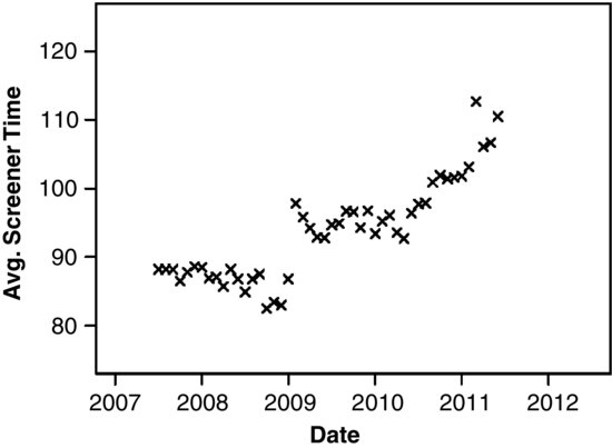
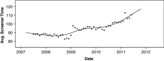
Each month, the Census Bureau gathers data from NCVS field operations and synthesizes them into variables that serve as indicators of data quality. One variable regarded as a key quality indicator is the duration of the screener interview. If the interviewer conducts the screener too quickly or in a careless fashion, some victimizations may go unreported, causing the estimated victimization rates to be artificially low. Figure 13.1 shows a plot of the average screener time reported monthly from July, 2007 (when Computer-Assisted Personal Interviewing (CAPI) became the standard data collection mode) to June, 2011. The series exhibits a slight decline through 2007 and 2008, a sharp increase early in 2009, a leveling off until mid-2010, and a steady increase thereafter.
FIGURE 13.1 Average time of screener interview in seconds for the National Crime Victimization Survey from July, 2007 to June, 2011.
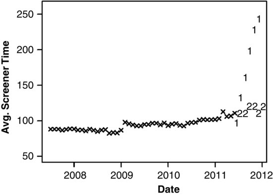
Midway through 2011, an intervention was begun to retrain the Census field to improve the quality of the NCVS interviews. One of the expected outcomes of this so-called Refresher Training was an increase in the average screener interview time. Refresher Training was introduced in a staggered fashion. Teams of interviewers were randomly assigned to two cohorts of roughly equal size. Cohort 1 received Refresher Training beginning in July 2011, and Cohort 2 received the same training in early 2012. Differences between the two cohorts during the last two quarters of 2011 may be used to estimate the effects of the training. A plot of the average screener times through the training period is shown in Figure 13.2, with observations for the cohorts denoted by plotting symbols “1” and “2.” As one might expect, Cohort 2 continues on a trajectory consistent with the series prior to July 2011, but Cohort 1 exhibits a sharp increase. After Cohort 2 receives the training during the first quarter of 2012, the two streams of data should (at least approximately) coalesce back into a single series.
FIGURE 13.2 Average time of screener interview in seconds for the National Crime Victimization Survey from July, 2007 to present, with classification by Refresher Training cohort (1 = training begun in July 2011, 2 = training deferred to 2012).
Given a data quality indicator series like the one shown in Figure 13.1, one can imagine many questions that may be posed by survey managers. For example:
- The value for this month seems unusually high. Given the trends and variability seen in the past, is this month's value outside of the range of what should be considered normal?
- This variable appears to have been stable (neither increasing nor decreasing) for the last 2 years, but the most recent measurements show a decline. Is this downward trend real, or could it be noise?
- December can be a difficult month for interviewing. How does the estimated mean value for December (averaged over multiple years) compare to the estimated mean value for January? Are they significantly different?
And given a branching series like the one shown in Figure 13.2, one could ask:
- What is the difference between the cohorts at a given month?
- What is the average difference between the cohorts over the past several months?
- After a specified number of months, have the two series joined back together? At what time is the difference between them no longer statistically significant?
To address questions like these, I propose a class of models based on penalized splines. These models will enable us to draw inferences about the mean of a process at any given time, the average of the process over a period of time, and the instantaneous change (slope) of the mean at any given time. The models also provide forecasts and prediction intervals for future observations. These models are intended to help managers monitor the performance of field staff, to describe the effects of interventions on the data collection process, and to quickly alert managers to unexpected developments that that may require remedial action.
13.1.3 Looking Ahead
In Section 13.2, I will review some key features of splines and describe their application to data series like the ones shown in Figures 13.1 and 13.2. In Section 13.3, I show how to fit smooth spline curves by characterizing them as linear mixed models and estimating the parameters by maximum likelihood (ML). ML gives reasonable estimates for the underlying trend, but the potentially unusual shape of the likelihood function makes the standard likelihood-based measures of uncertainty unreliable. In Section 13.4, I apply Markov chain Monte Carlo to simulate Bayesian estimates and intervals for a variety of interesting summaries. Computational details are provided in the Appendix.
The penalized splines in this chapter are intended to serve as a first generation of descriptive models for NCVS data-quality indicators. Looking ahead, we intend to expand these models to include effects of geography (e.g., Census Bureau Regional Offices) and interviewers as part of a more comprehensive paradata monitoring system. Those extensions are briefly mentioned in Section 13.5.
13.2 OVERVIEW OF SPLINES
13.2.1 Definition
Consider a data series ![]() ,
, ![]() , where
, where ![]() is a real-valued characteristic recorded at time
is a real-valued characteristic recorded at time ![]() . Let us suppose that
. Let us suppose that
where ![]() is an unknown function, and the residual errors are assumed to be independent and normally distributed with constant variance,
is an unknown function, and the residual errors are assumed to be independent and normally distributed with constant variance, ![]() . We believe that
. We believe that ![]() is continuous and fairly smooth, but the overall shape or form of this function is not specified in advance. Models of this form are described as semiparametric regression, local regression, or varying-coefficient models, and strategies for fitting them are described by Fan and Gijbels (1996); Green and Silverman (1994); Hastie and Tibshirani (1990); Wand and Jones (1995) and others. Many of these strategies are based on splines.
is continuous and fairly smooth, but the overall shape or form of this function is not specified in advance. Models of this form are described as semiparametric regression, local regression, or varying-coefficient models, and strategies for fitting them are described by Fan and Gijbels (1996); Green and Silverman (1994); Hastie and Tibshirani (1990); Wand and Jones (1995) and others. Many of these strategies are based on splines.
To formulate a spline, the span of the recorded times ![]() is partitioned into
is partitioned into ![]() intervals,
intervals,
![]()
and the interval cutpoints ![]() are called knots. Within each of the
are called knots. Within each of the ![]() intervals the function f is approximated by a polynomial of degree
intervals the function f is approximated by a polynomial of degree ![]() , and the polynomials are constrained so that f and its first
, and the polynomials are constrained so that f and its first ![]() derivatives agree at the knots.
derivatives agree at the knots.
An artificial bivariate dataset with spline fits of varying degrees is shown in Figure 13.3.
FIGURE 13.3 Artificial bivariate dataset with spline fits of varying degrees: (a) linear, (b) quadratic, (c) cubic, and (d) natural quadratic.
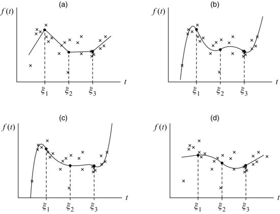
Each of these splines has ![]() knots. The spline shown in Figure 13.3a is a piecewise linear function, and the abrupt changes in slope give it a jagged appearance. The quadratic spline shown in Figure 13.3b is smoother because it is comprised of quadratic pieces whose slopes agree at the knots. The cubic spline in Figure 13.3c has continuous slope and curvature and looks even smoother. Ruppert et al. (2003) indicate that quadratic and cubic splines, while more aesthetically pleasing, may not perform much better than linear splines for estimating
knots. The spline shown in Figure 13.3a is a piecewise linear function, and the abrupt changes in slope give it a jagged appearance. The quadratic spline shown in Figure 13.3b is smoother because it is comprised of quadratic pieces whose slopes agree at the knots. The cubic spline in Figure 13.3c has continuous slope and curvature and looks even smoother. Ruppert et al. (2003) indicate that quadratic and cubic splines, while more aesthetically pleasing, may not perform much better than linear splines for estimating ![]() . If the model is used solely for prediction, linear splines may be smooth enough. For inferences about rates of change, however, splines of degree
. If the model is used solely for prediction, linear splines may be smooth enough. For inferences about rates of change, however, splines of degree ![]() are recommended, because a linear spline's instantaneous shifts in slope make estimates of
are recommended, because a linear spline's instantaneous shifts in slope make estimates of ![]() noisy.
noisy.
Quadratic, cubic and higher-degree splines may not provide reasonable estimates of ![]() for outlying values of t. In the curves shown in Figures 13.3b and c, it is apparent that the observations near the beginning and end of the series exert high leverage. The fitted curve swings sharply toward these initial and final observations and then continues on an implausible trajectory outside the range of the observed data, making predictions in those regions unstable. Figure 13.3d shows a quadratic spline that is constrained to be linear outside the boundary knots (i.e., where
for outlying values of t. In the curves shown in Figures 13.3b and c, it is apparent that the observations near the beginning and end of the series exert high leverage. The fitted curve swings sharply toward these initial and final observations and then continues on an implausible trajectory outside the range of the observed data, making predictions in those regions unstable. Figure 13.3d shows a quadratic spline that is constrained to be linear outside the boundary knots (i.e., where ![]() and
and ![]() ). Splines that are forced to be linear beyond the boundary knots are called natural splines. The natural quadratic spline shown in Figure 13.3d achieves a nice balance between smoothness and stability of forecasts.
). Splines that are forced to be linear beyond the boundary knots are called natural splines. The natural quadratic spline shown in Figure 13.3d achieves a nice balance between smoothness and stability of forecasts.
13.2.2 Basis Functions
One attractive feature of splines is that they can be cast within a framework of linear regression. For the linear spline shown in Figure 13.3a, the model was defined as
![]()
where
![]()
and ![]() ,
, ![]() ,
, ![]() ,
, ![]() , and
, and ![]() were estimated by ordinary least squares (OLS). In this model,
were estimated by ordinary least squares (OLS). In this model, ![]() and
and ![]() represent the intercept and slope of
represent the intercept and slope of ![]() for
for ![]() , and
, and ![]() is the change in slope at
is the change in slope at ![]() for
for ![]() .
.
More generally, a spline of degree ![]() with knots at
with knots at ![]() can be written as
can be written as
(13.2) ![]()
where
![]()
The set of ![]() functions
functions
![]()
is called the truncated power basis. Any ![]() th degree spline with knots at
th degree spline with knots at ![]() can be expressed as a linear combination of these functions. Given a series of observations
can be expressed as a linear combination of these functions. Given a series of observations ![]() , we can fit a spline model by computing the basis functions from the
, we can fit a spline model by computing the basis functions from the ![]() 's and regressing the
's and regressing the ![]() 's on those functions.
's on those functions.
The truncated power basis is easy to understand and implement, but it has some disadvantages. These basis functions tend to be highly correlated, and naive methods for performing least-squares computations on them may be poorly conditioned. Other sets of basis functions (e.g., B-splines) provide certain computational advantages, but their definition is more obscure. For most regression software programs in use today, multicollinearity is not a major concern, because internal routines will orthogonalize the regressors automatically.
We can modify a truncated power basis to force f to be linear beyond the boundary knots. Consider the quadratic spline
(13.3) ![]()
The first derivative of this function is
![]()
and the second derivative (which exists everywhere except the knots) is
![]()
where ![]() is an indicator function equal to one if its argument is true and zero otherwise. To require
is an indicator function equal to one if its argument is true and zero otherwise. To require ![]() for
for ![]() and
and ![]() , we need to set
, we need to set ![]() and
and ![]() . Substituting
. Substituting ![]() and
and ![]() into Equation (13.3), we see that the natural quadratic spline can be expressed as a linear combination of
into Equation (13.3), we see that the natural quadratic spline can be expressed as a linear combination of ![]() basis functions,
basis functions,
(13.4) ![]()
13.2.3 Parameters of Interest
Another attractive feature of spline models is that many interesting features of the fitted curve can be expressed as linear functions of regression coefficients. Statistical inferences about these features can be accomplished by computing estimates and measures of uncertainty for the unknown coefficients.
Consider a regression model based on the natural quadratic spline Equation 13.4. To compute the predicted value of the process at any time t, we simply plug that value of t and estimates for the β's and u's into the right-hand side of Equation 13.4.
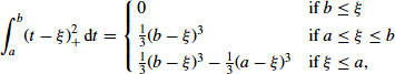
The average value of the process over the period of time from ![]() to
to ![]() is
is
![]()
as shown in Figure 13.4a. For the natural quadratic spline Equation 13.4, this process average becomes
![]()
where
which is a linear combination of the β's and u's.
FIGURE 13.4 Summaries of a natural quadratic spline: (a) average of the function from ![]() to
to ![]() , (b) first derivative of the function, and (c) average of the first derivative from
, (b) first derivative of the function, and (c) average of the first derivative from ![]() to
to ![]() .
.
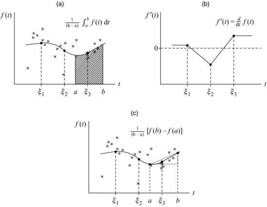
The first derivative of the natural quadratic spline function is
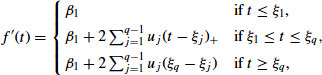
which again is a linear combination β's and u's. This derivative, as shown in Figure 13.4b, is piecewise linear between the interior knots and piecewise constant outside the boundary knots. To detect whether the process is trending upward or downward at any time t, we would compute confidence limits for ![]() to see if the interval covers zero.
to see if the interval covers zero.
It may also be of interest to determine whether the process has been trending upward or downward over a period of time. The average first derivative from ![]() to
to ![]() is
is
![]()
as shown in Figure 13.4c. Once again, this is a linear combination of β's and u's.
13.2.4 Branching Splines
Splines can also be used to describe a data series like the one shown in Figure 13.2 which branches into multiple series. Consider a natural quadratic spline with knots placed at ![]() . Suppose that it branches in the following manner. For
. Suppose that it branches in the following manner. For ![]() , we have a single function
, we have a single function ![]() . At
. At ![]() , the function splits into quadratic splines
, the function splits into quadratic splines ![]() and
and ![]() which are continuous with
which are continuous with ![]() and whose first derivatives are also continuous with
and whose first derivatives are also continuous with ![]() . Finally, suppose that
. Finally, suppose that ![]() ,
, ![]() , and
, and ![]() are linear outside the boundary knots
are linear outside the boundary knots ![]() and
and ![]() . This natural quadratic branching spline may be expressed as
. This natural quadratic branching spline may be expressed as
(13.5) 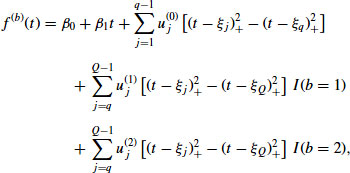
where ![]() denotes the branch. A spline with these properties is shown in Figure 13.5a.
denotes the branch. A spline with these properties is shown in Figure 13.5a.
FIGURE 13.5 (a) Natural quadratic spline which splits into two branches. (b) Average difference between branches from ![]() to
to ![]() .
.
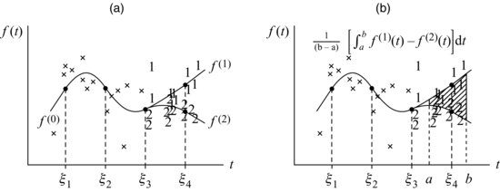
With a branching spline, we may be primarily interested in the difference between ![]() and
and ![]() . At any point
. At any point ![]() , we may compute confidence limits for
, we may compute confidence limits for ![]() to determine if this quantity is significantly different from zero. We may also be interested in the average difference over an interval from
to determine if this quantity is significantly different from zero. We may also be interested in the average difference over an interval from ![]() and
and ![]() ,
,
![]()
as shown in Figure 13.5b.
In a branching spline regression model, the assumption that residuals have constant variance may need to be modified. For the NCVS Refresher Training experiment described in Section 13.1.2, interviewers were assigned to two cohorts of roughly the same size. Let ![]() denote an observation at time
denote an observation at time ![]() , where
, where ![]() for the period before the experiment began,
for the period before the experiment began, ![]() for Cohort 1, and
for Cohort 1, and ![]() for Cohort 2. The sample sizes associated with
for Cohort 2. The sample sizes associated with ![]() and
and ![]() are about half of the sample size associated with
are about half of the sample size associated with ![]() . Therefore, in this example it is reasonable to suppose that
. Therefore, in this example it is reasonable to suppose that
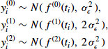
for some unknown ![]() . More generally, we may assume
. More generally, we may assume ![]() , where the
, where the ![]() 's are known constants.
's are known constants.
13.2.5 Knot Density and Roughness
The performance of a spline is affected by the number and location of the knots. If knots are too sparse, the fitted curve may fail to capture important trends in the data. Placing knots at frequent, regular intervals produce a flexible model that can accommodate virtually any kind of trend. However, if the model has a large number of knots and the coefficents are estimated by OLS, the function may be overfitted; the estimated curve will exhibit too many short-term increases and decreases in response to random noise. Although there are no hard and fast rules choosing the number of knots, Ruppert et al. (2003, p. 126) suggest that a reasonable default number is
![]()
For a monthly series less than 12 years in length, this rule suggests using one knot for every 4 months (three per year). Because certain results from NCVS are compiled and reviewed on a quarterly basis, it seems reasonable for us to place knots at the beginning of every quarter.
Returning to the NCVS screener time data shown in Figure 13.1, we placed knots at the beginning of each quarter (![]() ) and fit a natural quadratic spline by OLS. The result is shown in Figure 13.6, with an expanded time axis for greater clarity. The estimated function is wiggly, with numerous brief upswings and dips that probably reflect random variation, not actual trends.
) and fit a natural quadratic spline by OLS. The result is shown in Figure 13.6, with an expanded time axis for greater clarity. The estimated function is wiggly, with numerous brief upswings and dips that probably reflect random variation, not actual trends.
FIGURE 13.6 Average time of screener interview for the National Crime Victimization Survey, with a natural quadratic spline fit by OLS.

The curve shown in Figure 13.6 could be made smoother by eliminating some of the knots. For example, one could imagine a stepwise procedure that removes from the model Equation 13.4 the basis functions for u's that are not significantly different from zero. However, stepwise procedures have some serious drawbacks. When the basis functions are highly multicollinear, small fluctuations in the data and small changes in stepwise decision rules could lead to substantially different models. Moreover, with stepwise methods it is difficult to obtain honest confidence intervals that reflect the randomness in the outcome of the variable-selection procedure.
Instead of eliminating knots by setting some of the u's to zero, suppose that we retain all of the knots and shrink all of the u's partway toward zero. This is accomplished by changing the fitting criterion. An OLS procedure estimates the β's and u's by minimizing the residual sum of squares
![]()
If we modify this criterion by adding to RSS a roughness penalty, a term that increases as the curve becomes more wiggly, the resulting ![]() is called a penalized spline. The literature on penalized splines is quite extensive, and a good overview is provided by Ruppert et al. (2003, Chapter 5). One way to implement a roughness penalty is to apply a probability distribution to the u-coefficients, transforming the spline into a linear mixed model. This is the subject of Section 13.3.
is called a penalized spline. The literature on penalized splines is quite extensive, and a good overview is provided by Ruppert et al. (2003, Chapter 5). One way to implement a roughness penalty is to apply a probability distribution to the u-coefficients, transforming the spline into a linear mixed model. This is the subject of Section 13.3.
13.3 PENALIZED SPLINES AS LINEAR MIXED MODELS
13.3.1 Model Formulation
Suppose we construct a spline with a truncated power basis as in Equations 13.2, 13.4, or 13.5. And suppose we regard the u-coefficients as independent and normally distributed,
(13.6) ![]()
This assumption transforms the regression spline into a linear mixed model with two variance components, ![]() and
and ![]() , which can both be estimated from the data. The random-effect distribution Equation 13.6 plays the role of a roughness penalty. The practical impact is that the estimated u's will be shrunk toward zero, with the degree of shrinkage determined by the relative sizes of the variance components. For example, consider the natural quadratic spline Equation 13.4. Maximum shrinkage
, which can both be estimated from the data. The random-effect distribution Equation 13.6 plays the role of a roughness penalty. The practical impact is that the estimated u's will be shrunk toward zero, with the degree of shrinkage determined by the relative sizes of the variance components. For example, consider the natural quadratic spline Equation 13.4. Maximum shrinkage ![]() will set the u's to zero, producing an OLS straight line fit to the observed data, whereas no shrinkage
will set the u's to zero, producing an OLS straight line fit to the observed data, whereas no shrinkage ![]() leads to a situation like that shown in Figure 13.6 where the u's and β's are simultaneously estimated by OLS. The mixed-model penalized spline produces a compromise between these two extremes.
leads to a situation like that shown in Figure 13.6 where the u's and β's are simultaneously estimated by OLS. The mixed-model penalized spline produces a compromise between these two extremes.
The linear mixed model can be expressed in matrix form as follows. Define the vector of observations ![]() and residual errors
and residual errors ![]() . Collect the basis functions corresponding to the β's into an
. Collect the basis functions corresponding to the β's into an ![]() matrix
matrix ![]() , and the basis functions corresponding to the u's into an
, and the basis functions corresponding to the u's into an ![]() matrix
matrix ![]() . For example, with the natural quadratic spline Equation 13.4, the matrices are
. For example, with the natural quadratic spline Equation 13.4, the matrices are
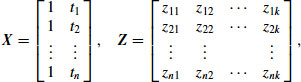
where
![]()
for ![]() . The model becomes
. The model becomes
where ![]() and
and ![]() , where
, where ![]() denotes the
denotes the ![]() identity matrix, and
identity matrix, and ![]() denotes an
denotes an ![]() diagonal matrix of known constants
diagonal matrix of known constants
![]()
In many cases we will take ![]() , but the more general diagonal form of
, but the more general diagonal form of ![]() is needed to accommodate situations like the branching spline described in Section 13.2.4 where the measurements for the branches
is needed to accommodate situations like the branching spline described in Section 13.2.4 where the measurements for the branches ![]() and
and ![]() have higher variance than the measurements for
have higher variance than the measurements for ![]() .
.
The parameters to be estimated in this model are the fixed coefficients ![]() and the variance components
and the variance components ![]() . It will be computationally convenient to work with the ratio
. It will be computationally convenient to work with the ratio ![]() which is called a smoothing parameter, because it determines the degree of smoothness in the fitted function. As
which is called a smoothing parameter, because it determines the degree of smoothness in the fitted function. As ![]() , the estimated f approaches an OLS spline as shown in Figure 13.6, and as
, the estimated f approaches an OLS spline as shown in Figure 13.6, and as ![]() , it approaches an OLS straight line fit to the entire data series.
, it approaches an OLS straight line fit to the entire data series.
13.3.2 Estimating Parameters
Commercially available software packages (e.g., Proc MIXED in SAS) are capable of fitting normal linear mixed models. For our purposes, we have developed custom routines which take advantage of the particular covariance structure of this model and which may be extended in the future to more complicated situations for which no software is readily available (e.g., models with interviewer effects).
Model Equation 13.7 implies that
where ![]() , and where
, and where ![]() denotes the unknown parameters. Note that
denotes the unknown parameters. Note that ![]() depends on
depends on ![]() but not
but not ![]() or
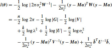
or ![]() . The likelihood function associated with Equation 13.8 is
. The likelihood function associated with Equation 13.8 is
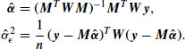
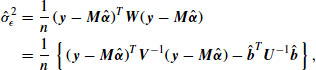
For any fixed value of ![]() , this function is maximized at the generalized least squares (GLS) estimates
, this function is maximized at the generalized least squares (GLS) estimates
Substituting these estimates into ![]() produces a function of the single variable
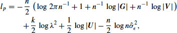
produces a function of the single variable ![]() whose maximizer will maximize the loglikelihood. This new function, which is called the profile loglikelihood, is
whose maximizer will maximize the loglikelihood. This new function, which is called the profile loglikelihood, is
(13.12) ![]()
where ![]() is an additive constant that may be ignored. The maximizer of
is an additive constant that may be ignored. The maximizer of ![]() cannot be written in closed form but must be computed by an iterative method. In Appendix A.1, we describe an extension of the EM algorithm which is very stable, has a low per-iteration cost, and converges reliably to a (possibly local) maximum.
cannot be written in closed form but must be computed by an iterative method. In Appendix A.1, we describe an extension of the EM algorithm which is very stable, has a low per-iteration cost, and converges reliably to a (possibly local) maximum.
13.3.3 Estimating the Function
Once the estimated parameters ![]() are available, we can estimate the curve as follows. The spline function at time t can be written as
are available, we can estimate the curve as follows. The spline function at time t can be written as
(13.13) ![]()
where ![]()
![]() and
and ![]()
![]() are known vectors of basis functions that depend on t. For example, in the natural quadratic spline model Equation 13.4, the vectors are
are known vectors of basis functions that depend on t. For example, in the natural quadratic spline model Equation 13.4, the vectors are
![]()
Formally, we may view ![]() as the conditional mean given the random effects
as the conditional mean given the random effects ![]() and parameters
and parameters ![]() ,
,
![]()
and inferences about ![]() require us to simultaneously estimate
require us to simultaneously estimate ![]() and predict
and predict ![]() . The linear mixed model Equation 13.7 implies that
. The linear mixed model Equation 13.7 implies that ![]() and
and ![]() have a joint normal distribution,
have a joint normal distribution,
![]()
The implied conditional distribution for ![]() given
given ![]() is normal with mean vector and covariance matrix
is normal with mean vector and covariance matrix
(13.15) ![]()
where ![]() . Substituting the ML estimate
. Substituting the ML estimate ![]() for the unknown
for the unknown ![]() into Equation 14 produces an estimated best linear unbiased predictor (EBLUP) for
into Equation 14 produces an estimated best linear unbiased predictor (EBLUP) for ![]() ,
,
![]()
which can also be interpreted as an empirical Bayes (EB) estimator. The corresponding EB estimate for ![]() is
is
![]()
We used this procedure to fit a natural quadratic spline model to the NCVS screener times shown in Figure 13.1. Taking ![]() as the starting value, the EM algorithm converged in 237 iterations (convergence criterion
as the starting value, the EM algorithm converged in 237 iterations (convergence criterion ![]() ) to a final estimate of
) to a final estimate of ![]() . Plugging this value into Equations 10 and 11, we obtained
. Plugging this value into Equations 10 and 11, we obtained

The fitted curve implied by these estimates is shown in Figure 13.7.
FIGURE 13.7 Average time of screener interview for the National Crime Victimization Survey, with a natural quadratic penalized spline fit by maximum likelihood.
This new curve tracks the data series well, but is much less wiggly than the OLS curve.
13.3.4 Difficulties with Likelihood Inference
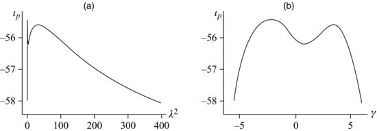
The ML procedure for estimating ![]() produces a reasonable answer for the NCVS screener time series. Upon close examination, however, some difficulties come to light. A plot of the profile loglikelihood function
produces a reasonable answer for the NCVS screener time series. Upon close examination, however, some difficulties come to light. A plot of the profile loglikelihood function ![]() over a range of
over a range of ![]() values is shown in Figure 13.8a. This function is unusually shaped; it has a sharp spike located near
values is shown in Figure 13.8a. This function is unusually shaped; it has a sharp spike located near ![]() , another peak for larger values of
, another peak for larger values of ![]() , and a very long tail on the right-hand side. The picture becomes clearer if we transform
, and a very long tail on the right-hand side. The picture becomes clearer if we transform ![]() to the log scale, and in Figure 13.8b we replotted
to the log scale, and in Figure 13.8b we replotted ![]() a function of
a function of ![]() . One peak is located at
. One peak is located at ![]() , the estimate that we obtained from EM. But a second peak occurs at
, the estimate that we obtained from EM. But a second peak occurs at ![]() , and if we had run the EM algorithm with a larger starting value, we would have converged to that second answer. The profile loglikelihood at the first solution is higher, so
, and if we had run the EM algorithm with a larger starting value, we would have converged to that second answer. The profile loglikelihood at the first solution is higher, so ![]() is indeed the ML estimate. But the difference in
is indeed the ML estimate. But the difference in ![]() is so slight that it gives us almost no evidence to prefer either of the two solutions.
is so slight that it gives us almost no evidence to prefer either of the two solutions.
FIGURE 13.8 Profile loglikelihood function for natural quadratic penalized spline fit to average screener times, plotted (a) as a function of the smoothing parameter ![]() and (b) as a function of
and (b) as a function of ![]() .
.
In fact, this likelihood suggests that a wide range of ![]() values is consistent with the data. By a standard likelihood-ratio test, any value of
values is consistent with the data. By a standard likelihood-ratio test, any value of ![]() for which
for which ![]() cannot be rejected at the 0.05 level. By this criterion, an approximate 95% confidence interval for
cannot be rejected at the 0.05 level. By this criterion, an approximate 95% confidence interval for ![]() ranges from 0.00583 to 262. But the unusual shape of
ranges from 0.00583 to 262. But the unusual shape of ![]() in this example serves as a warning that the standard large-sample approximations used in likelihood inference are problematic. To develop reliable measures of uncertainty for the fitted function and related quantities, we now turn to Bayesian methods.
in this example serves as a warning that the standard large-sample approximations used in likelihood inference are problematic. To develop reliable measures of uncertainty for the fitted function and related quantities, we now turn to Bayesian methods.
13.4 BAYESIAN METHODS
13.4.1 Bayesian Inference for the Smoothing Parameter
Bayesian inference for linear mixed models has become commonplace since the advent of Markov chain Monte Carlo (MCMC) (Gelman et al., 2004). Perhaps the simplest strategy for Bayesian inference in this model would be to iteratively simulate random draws of ![]() by a Gibbs sampler that augments the observed data
by a Gibbs sampler that augments the observed data ![]() with simulated values for the random coefficients
with simulated values for the random coefficients ![]() at each cycle. We experimented with Gibbs samplers for the NCVS screener data series and found that they converged very slowly, prompting us to search for more efficient alternatives.
at each cycle. We experimented with Gibbs samplers for the NCVS screener data series and found that they converged very slowly, prompting us to search for more efficient alternatives.
The only real difficulty in this model comes from the smoothing parameter ![]() . Suppose we condition on
. Suppose we condition on ![]() and apply a standard noninformative prior distribution to
and apply a standard noninformative prior distribution to ![]() and
and ![]() ,
,
![]()
which supposes that ![]() and the elements of
and the elements of ![]() are uniformly distributed over the real line. Under this prior, the conditional posterior distribution for
are uniformly distributed over the real line. Under this prior, the conditional posterior distribution for ![]() given
given ![]() becomes the product of (a) a scaled inverted chisquare distribution for
becomes the product of (a) a scaled inverted chisquare distribution for ![]() and (b) a multivariate normal distribution for
and (b) a multivariate normal distribution for ![]() given
given ![]() . Formulas for these posterior distributions are provided in Appendices A.2 and A.3.
. Formulas for these posterior distributions are provided in Appendices A.2 and A.3.
Taking advantage of this tractability if ![]() were known, we developed a Metropolis–Hastings algorithm that simulates random draws of
were known, we developed a Metropolis–Hastings algorithm that simulates random draws of ![]() from its marginal posterior distribution. Details of this algorithm are given in Appendix A.2. We applied a very diffuse prior distribution, supposing that
from its marginal posterior distribution. Details of this algorithm are given in Appendix A.2. We applied a very diffuse prior distribution, supposing that ![]() for
for ![]() and
and ![]() . Taking the ML estimate as a starting value, we generated a sequence of 10,000 draws of
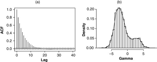
. Taking the ML estimate as a starting value, we generated a sequence of 10,000 draws of ![]() . The sample autocorrelation function (ACF) for this series is shown in Figure 13.9a. The autocorrelation becomes insignificant by lag 15, indicating that the Metroplis–Hastings procedure converges rapidly. (By contrast, for the Gibbs samplers that we examined, autocorrelations remained high even after several hundred cycles.) A histogram and density estimate for the 10,000 draws of
. The sample autocorrelation function (ACF) for this series is shown in Figure 13.9a. The autocorrelation becomes insignificant by lag 15, indicating that the Metroplis–Hastings procedure converges rapidly. (By contrast, for the Gibbs samplers that we examined, autocorrelations remained high even after several hundred cycles.) A histogram and density estimate for the 10,000 draws of ![]() are shown in Figure 13.9b. Comparing this histogram to the profile loglikelihood in Figure 13.8b, we notice that the posterior probability is now concentrated near the major mode of the likelihood function, and support for values near the minor mode has diminished.
are shown in Figure 13.9b. Comparing this histogram to the profile loglikelihood in Figure 13.8b, we notice that the posterior probability is now concentrated near the major mode of the likelihood function, and support for values near the minor mode has diminished.
FIGURE 13.9 (a) Sample for a sequence of 10,000 draws of ![]() from Metroplis–Hastings. (b) Histogram and density estimate for posterior draws of
from Metroplis–Hastings. (b) Histogram and density estimate for posterior draws of ![]() .
.
13.4.2 Bayesian Intervals and Predictions
Conditional upon the smoothing parameter, any linear combination of ![]() and
and ![]() has a Student's t posterior distribution. Using this fact, we obtained Bayesian estimates for
has a Student's t posterior distribution. Using this fact, we obtained Bayesian estimates for ![]() by a Rao–Blackwell method which computes the posterior mean for each simulated value of
by a Rao–Blackwell method which computes the posterior mean for each simulated value of ![]() and averages them over the simulated values. Posterior intervals for
and averages them over the simulated values. Posterior intervals for ![]() and prediction intervals for future observations can be obtained in a similar fashion; details are given in Appendix A.3.
and prediction intervals for future observations can be obtained in a similar fashion; details are given in Appendix A.3.
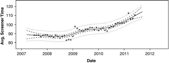
A plot of the Bayes estimate of ![]() for the NCVS screener time series is shown in Figure 13.10. The estimated function (solid line) is nearly indistinguishable from the ML curve shown in Figure 13.7. Along the Bayesian curve, we are also able to show 95% intervals for
for the NCVS screener time series is shown in Figure 13.10. The estimated function (solid line) is nearly indistinguishable from the ML curve shown in Figure 13.7. Along the Bayesian curve, we are also able to show 95% intervals for ![]() (dashed lines) and prediction intervals for future observations (dotted lines).
(dashed lines) and prediction intervals for future observations (dotted lines).
FIGURE 13.10 Simulated Bayes estimate of the mean function from the NCVS screener time series (solid line), with 95% intervals for the mean function (dashed lines) and 95% prediction intervals for future observations (dotted lines).
Because integrals and derivatives of ![]() are also linear combinations of
are also linear combinations of ![]() and
and ![]() , estimates and intervals for these quantities can be computed in a similar fashion. Estimates and intervals for the first derivative
, estimates and intervals for these quantities can be computed in a similar fashion. Estimates and intervals for the first derivative ![]() are shown in Figure 13.11.
are shown in Figure 13.11.
Figure 13.11 Simulated Bayes estimate of the first derivative of the mean function from the NCVS screener time series (solid line) with 95% intervals (dashed lines).
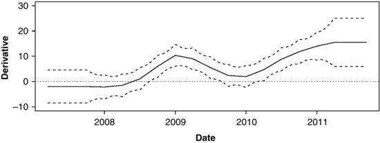
Convincing evidence of a trend is found wherever the interval does not cover zero. The gradual downward trend in the first year (prior to mid-2008) is not statistically significant. But the rapid increase at the beginning of 2009 is significant, and so is the sustained increase after mid-2010.
By changing the basis functions, the same procedures may be used to obtain Bayesian estimates and intervals for branching splines. An estimated branching spline for the two cohorts in the NCVS refresher training experiment in shown in Figure 13.12.
FIGURE 13.12 Bayes estimate for a branching spline fit to the screener times in the NCVS refresher training experiment.
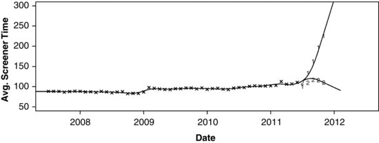
Knots are placed at the beginning of each quarter, and the branching knot is placed at July, 2011 when the experiment began. The divergence of the two cohorts is dramatic and obviously significant. The estimated difference between the two curves (Cohort 1 − Cohort 2) after July 2011 is plotted in Figure 13.13, along with 95% intervals.
FIGURE 13.13 Estimated difference between Cohorts 1 and 2 in the NCVS refresher training experiment (solid line) with 95% intervals (dashed lines).
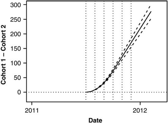
Because this model forces the two curves to agree at the branching knot, the estimated effect for July, 2011 is constrained to be zero. The estimated difference between the curves at the subsequent months are shown in Table 13.1, along with 95% intervals.
Table 13.1 Estimated Difference in Average Screener Interview Times Between Cohorts 1 and 2, with 95% Intervals
| Month | Estimate | 95% Interval |
| 7/11 | 0.00 | (0.00, 0.00) |
| 8/11 | 2.91 | (2.65, 3.17) |
| 9/11 | 11.63 | (10.60, 12.66) |
| 10/11 | 26.17 | (23.86, 28.49) |
| 11/11 | 46.53 | (42.42, 50.64) |
| 12/11 | 72.70 | (66.28, 79.13) |
13.5 EXTENSIONS
This chapter was intended to serve as an introduction to the use of penalized splines for describing and monitoring a paradata series. The models presented here are designed for a single variable recorded over time at regular or irregular intervals. The assumption of a normally distributed residual error might be appropriate for a continuous numeric variable such as the average NCVS screener times. For a numeric variable that is highly skewed, or for an outcome measure that represents a count, proportion or rate, it becomes advantageous to generalize our model Equation 13.1 to
![]()
where F is a parametric family of distributions with mean ![]() and dispersion parameter
and dispersion parameter ![]() , and then assume
, and then assume
![]()
where g is a known monotonic link function. In a future article, we will investigate these more general models where F includes the binomial, beta, Poisson, gamma, beta-binomial, and negative binomial families. One disadvantage of moving to a non-normal F is that some of the elegance and speed of the algorithms described in the Appendix are lost; ML becomes substantially more difficult, and in general we can no longer analytically integrate over the random coefficients or the dispersion parameter. Inference by MCMC is still possible, however, and strategies that are well known in the Bayesian literature (e.g., Gibbs samplers with embedded steps of Metropolis–Hastings) are straightforward to implement in principle, although in practice they require considerable care and fine tuning to work well.
In addition to using non-normal families, we are also extending the model to multilevel or nested datasets where, at each occasion, the outcome variable is recorded at multiple units of observation. Those observational units may be geographic regions (e.g., Regional Offices), managerial teams, interviewers, or all of the above. The mixed-effect regression formulation of our spline model generalizes in a straightforward way to hierarchical or nested data structures, although the algorithms for fitting these models are not well developed. Penalized spline models for nested observational units are described by Wu and Zhang (2006); Welham (2008); Brumback et al. (2008).
APPENDIX
A.1 Maximum-likelihood Estimation
Consider the linear mixed model
![]()
where ![]() and
and ![]() . Although we assume that
. Although we assume that ![]() and
and ![]() have full rank, the functions from a truncated power basis can make their columns nearly collinear, causing
have full rank, the functions from a truncated power basis can make their columns nearly collinear, causing ![]() and
and ![]() to be poorly conditioned. To help stabilize the computations, we begin by orthogonalizing
to be poorly conditioned. To help stabilize the computations, we begin by orthogonalizing ![]() and
and ![]() using a Gram–Schmidt procedure. That is, we decompose them as
using a Gram–Schmidt procedure. That is, we decompose them as ![]() and
and ![]() , where
, where ![]() and
and ![]() , and where
, and where ![]() and
and ![]() are upper triangular. The linear mixed model becomes
are upper triangular. The linear mixed model becomes
![]()
where ![]() ,
, ![]() , and
, and ![]() . Letting
. Letting ![]() and
and ![]() , we have
, we have
where ![]() .
.
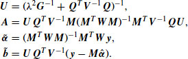
By the Sherman–Morrison–Woodbury formula and determinant lemma, we can write
![]()
where
![]()
These identities allow us to work with inverses and determinants of matrices that are ![]() rather than
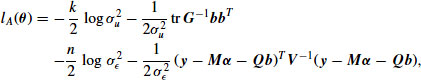
rather than ![]() . Applying these identities, the loglikelihood function for
. Applying these identities, the loglikelihood function for ![]() corresponding to Equation 13.16 may be written as
corresponding to Equation 13.16 may be written as
where ![]() . If
. If ![]() were known, we could immediately maximize
were known, we could immediately maximize ![]() with respect to the other parameters by GLS,
with respect to the other parameters by GLS,
Because ![]() and
and ![]() are functions of
are functions of ![]() , we can substitute
, we can substitute ![]() and
and ![]() into Equation 17, yielding the profile loglikelihood,
into Equation 17, yielding the profile loglikelihood,
which is a function of the single parameter ![]() . This profile loglikelihood tends to be better behaved (i.e., more nearly symmetric and quadratic) when viewed as a function of
. This profile loglikelihood tends to be better behaved (i.e., more nearly symmetric and quadratic) when viewed as a function of ![]() .
.
This function can be maximized in a variety of ways. One possibility is Newton--Raphson, which requires computation of the first two derivatives of ![]() with respect to
with respect to ![]() . Applying techniques of matrix calculus, the first derivative can be written as
. Applying techniques of matrix calculus, the first derivative can be written as
(13.19) ![]()
where
![]()
The second derivative can be expressed as
(13.20) 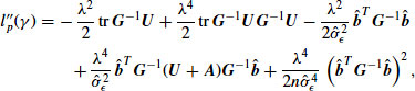
where
![]()
Newton--Raphson tends to work well when the starting value for ![]() is located in the vicinity of the maximizer
is located in the vicinity of the maximizer ![]() . In regions far from
. In regions far from ![]() , however,
, however, ![]() could be non-concave, causing the algorithm to fail.
could be non-concave, causing the algorithm to fail.
A more stable procedure for maximizing ![]() is motivated by an EM algorithm which treats the random effects as missing data. If
is motivated by an EM algorithm which treats the random effects as missing data. If ![]() could be observed, the augmented-data loglikelihood function would be
could be observed, the augmented-data loglikelihood function would be
![]()
which has a particularly simple form. Omitting additive constants, this function is
which is linear in ![]() and
and ![]() . Under an assumed value for
. Under an assumed value for ![]() , the expectation of
, the expectation of ![]() with respect to
with respect to ![]() is computed by replacing
is computed by replacing ![]() with
with ![]() and
and ![]() with
with ![]() . Consider a procedure in which we alternately (a) maximize
. Consider a procedure in which we alternately (a) maximize ![]() with respect to
with respect to ![]() and
and ![]() , fixing
, fixing ![]() at its current estimate, and (b) maximize the expected value of
at its current estimate, and (b) maximize the expected value of ![]() with respect to
with respect to ![]() , fixing
, fixing ![]() and
and ![]() at their current estimates. The resulting procedure is an extension of EM known as ECME (Liu and Rubin, 1995), and it has the same reliable convergence behavior as EM: each interaction is guaranteed to increase
at their current estimates. The resulting procedure is an extension of EM known as ECME (Liu and Rubin, 1995), and it has the same reliable convergence behavior as EM: each interaction is guaranteed to increase ![]() . One iteration of the algorithm may be expressed as follows. Given the starting estimate
. One iteration of the algorithm may be expressed as follows. Given the starting estimate ![]() , update the estimate by computing in the following order:
, update the estimate by computing in the following order:
(13.21) ![]()
(13.22) 
(13.23) ![]()
Between steps Equations 24 and 25, the loglikelihood at the starting estimate may be computed using Equation 18.
A.2 Posterior Simulation
To simulate values of parameters from a posterior distribution, we need to specify a prior density for ![]() . For our purposes, it is convenient to apply independent prior distributions to
. For our purposes, it is convenient to apply independent prior distributions to ![]() ,
, ![]() , and
, and ![]() . Suppose we apply an improper uniform prior density to
. Suppose we apply an improper uniform prior density to ![]() ,
,
(13.26) ![]()
a scaled inverted-chisquare distribution to ![]() ,
,
and a normal distribution to ![]() ,
,
(13.28) ![]()
where ![]() ,
, ![]() ,
, ![]() , and
, and ![]() are user-specified hyperparameters. In the typical situation where prior knowledge about
are user-specified hyperparameters. In the typical situation where prior knowledge about ![]() is vague, we may take the limiting form of Equation 13.27 as
is vague, we may take the limiting form of Equation 13.27 as ![]() and
and ![]() , which is equivalent to specifying an improper uniform density for
, which is equivalent to specifying an improper uniform density for ![]() over the real line. The implied joint prior density for
over the real line. The implied joint prior density for ![]() is
is
![]()
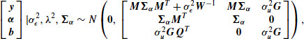
Combining this prior with the likelihood function Equation 13.9, the joint posterior density for ![]() becomes
becomes
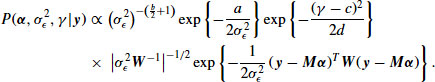
For a fixed value of ![]() , the conditional posterior distribution for
, the conditional posterior distribution for ![]() is
is
![]()
where
We may analytically integrate Equation 29 with respect to ![]() and
and ![]() , resulting in the marginal posterior density for
, resulting in the marginal posterior density for ![]() ,
,
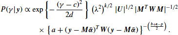
This is not a recognizable as any standard distribution, and the normalizing constant is unknown. However, it is possible to generate a sequence of random draws from ![]() by MCMC. Using a strategy suggested by Gelman et al. (2004), we implemented a Metropolis random walk as follows. Let
by MCMC. Using a strategy suggested by Gelman et al. (2004), we implemented a Metropolis random walk as follows. Let ![]() denote the simulated value at iteration
denote the simulated value at iteration ![]() . Draw a candidate value
. Draw a candidate value ![]() from a Student's t distribution with
from a Student's t distribution with ![]() degrees of freedom centered at
degrees of freedom centered at ![]() ,
,
![]()
where the scale is obtained by matching the second derivative of the Student's t density to that of the profile loglikelihood at the ML estimate ![]() ,
,
![]()
As a rule-of-thumb, Gelman et al. (2004) recommend taking ![]() . Compute the Metropolis acceptance ratio
. Compute the Metropolis acceptance ratio
![]()
which is possible because the unknown normalizing constant in Equation 30 cancels out. Then draw a uniform variate ![]() and take
and take
![]()
A.3 Bayesian Inference About the Mean Function
Consider the orthogonalized model
![]()
where ![]() and
and ![]() . In a typical Bayesian formulation of a linear mixed model, the “fixed effects”
. In a typical Bayesian formulation of a linear mixed model, the “fixed effects” ![]() are regarded as a random vector with a diffuse prior. If we specify a normal prior,
are regarded as a random vector with a diffuse prior. If we specify a normal prior,
![]()
and take the limit as ![]() , the result is an improper uniform prior density
, the result is an improper uniform prior density ![]() . Under this model, the response vector
. Under this model, the response vector ![]() and the coefficients
and the coefficients ![]() and
and ![]() have a joint normal distribution,
have a joint normal distribution,
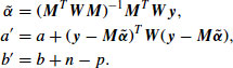
where ![]() . Using algebraic techniques described by Carlin (1990), one can show that, in the limit as
. Using algebraic techniques described by Carlin (1990), one can show that, in the limit as ![]() , the conditional posterior distribution of
, the conditional posterior distribution of ![]() given
given ![]() and the variance parameters is
and the variance parameters is
![]()
where ![]() ,
, ![]() ,
, ![]() , and
, and ![]() are functions of
are functions of ![]() and
and ![]() but not
but not ![]() ,
,
The joint posterior distribution of the untransformed coefficients ![]() and
and ![]() given the variance parameters follows by noting that
given the variance parameters follows by noting that
![]()
The mean function at an arbitrary time t can be written as
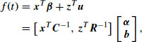
where ![]() and
and ![]() are vectors of basis functions that depend on t. Therefore, the conditional posterior distribution of
are vectors of basis functions that depend on t. Therefore, the conditional posterior distribution of ![]() given
given ![]() and the variance parameters is normal,
and the variance parameters is normal,
where
![]()
and
![]()
are functions of ![]() and
and ![]() but not
but not ![]() . Averaging the distribution Equation 13.31 over
. Averaging the distribution Equation 13.31 over ![]() , the posterior distribution for
, the posterior distribution for ![]() given
given ![]() and
and ![]() becomes a Student's t with
becomes a Student's t with ![]() degrees of freedom,
degrees of freedom,
![]()
where
![]()
Given a sequence of ![]() random (not necessarily independent) draws from the posterior distribution of
random (not necessarily independent) draws from the posterior distribution of ![]() , which can be generated as described in Appendix A.2,
, which can be generated as described in Appendix A.2,
![]()
a Rao–Blackwellized estimate of the posterior mean of ![]() is
is
(13.32) ![]()
and a Rao–Blackwellized estimate of the qth posterior quantile of ![]() is
is
(13.33) ![]()
where ![]() denotes the qth quantile of Student's t distribution with
denotes the qth quantile of Student's t distribution with ![]() degrees of freedom.
degrees of freedom.
By a similar argument, one can derive a Bayesian posterior prediction interval for an unseen future observation ![]() where
where ![]() . The posterior predictive distribution for
. The posterior predictive distribution for ![]() given
given ![]() and
and ![]() is
is
![]()
A Rao–Blackwellized estimate of the posterior predictive mean is
(13.34) ![]()
and a Rao–Blackwellized estimate of the qth posterior predictive quantile is
(13.35) ![]()
A.4 Disclaimer
This report is released to inform interested parties of ongoing research and to encourage discussion of work in progress. The views expressed are those of the author and not necessarily those of the U.S. Census Bureau. Correspondence should be address to Joseph L. Schafer, Center for Statistical Research and Methodology, U.S. Census Bureau, 4600 Silver Hill Rd., Washington, DC, 20233, or [email protected].
REFERENCES
Biemer, P. (2010). Total Survey Error: Design, Implementation and Evaluation. Pubic Opinion Quarterly, 74:817–848.
Brumback, B., Brumback, L., and Lindstrom, M. (2008). Penalized Spline Models for Longitudinal Data. In Fitzmaurice, G., editor, Longitudinal Data Analysis: A Handbook of Modern Statistical Methods, pages 291–316. Chapman and Hall.
Couper, M. (1998). Measuring Survey Quality in a CASIC Environment. Proceedings of the Survey Research Methods Section, ASA, pages 41–49.
del Castillo, E. (2002). Statistical Process Adjustment for Quality Control. John Wiley and Sons.
Fan, J. and Gijbels, I. (1996). Local Polynomial Modelling and its Applications. Chapman and Hall.
Gelman, A., Rubin, D., Carlin, J., and Stern, H. (2004). Bayesian Data Analysis. 2nd edition. Chapman and Hall/CRC Press.
Green, P. and Silverman, B. (1994). Nonparametric Regression and Generalized Linear Models: A Roughness Penalty Approach. Chapman and Hall.
Groves, R.M. and Heeringa, S.G. (2006). Responsive Design for Household Surveys: Tools for Actively Controlling Survey Nonresponse and Costs. Journal of the Royal Statistical Society, Series A, 169(3):439–457.
Hastie, T. and Tibshirani, R. (1990). Generalized Additive Models. Chapman and Hall.
Liu, C. and Rubin, D. (1995). Application of the ECME Algorithm and the Gibbs Sampler to General Linear Mixed Models. Proceedings of the17th International Biometric Conference, 1:97–107.
Montgomery, D. (1996). Introduction to Statistical Quality Control. 3rd edition. John Wiley and Sons.
Ruppert, D., Wand, M., and Carrol, R. (2003). Semiparametric Regression. Cambridge University Press.
Shewhart, W. (1931). Economic Control of Quality of Manufactured Product. van Nostrand Reinhold Co., Princeton, NJ.
Wand, M. and Jones, M. (1995). Kernel Smoothing. Chapman and Hall.
Welham, S. (2008). Smoothing Spline Models for Longitudinal Data. In Fitzmaurice, G., editor, Longitudinal Data Analysis: A Handbook of Modern Statistical Methods, pages 253–289. Chapman and Hall.
Wheeler, D. and Chambers, D. (1992). Understanding Statistical Process Control. 2nd edition. SPC Press.
Wu, H. and Zhang, J.-T. (2006). Nonparametric Regression Methods for Longitudinal Data Analysis. John Wiley and Sons.