CHAPTER 12

MODELING CALL RECORD DATA: EXAMPLES FROM CROSS-SECTIONAL AND LONGITUDINAL SURVEYS

GABRIELE B. DURRANT and JULIA D’ARRIGO

Southampton Statistical Sciences Research Institute (S3RI), University of Southampton, UK

GERRIT MÜLLER

Institute for Employment Research (IAB), Nuremberg

12.1 INTRODUCTION

One class of paradata is interviewer call record data, sometimes referred to as call history data (Sangster and Meekins, 2004; Bates et al., 2008; Lee et al., 2009; Durrant et al., 2010; Blom et al., 2010; Durrant et al., 2013). Call record data is collected in interviewer-administered surveys, including both face-to-face and telephone surveys. Such data contain, for example, information about the day and time of the call to a sample unit and the outcome of the call. Further characteristics of the call may be captured, such as voice characteristics and initial responses from the householder or observational data about the household in face-to-face surveys. Call data may be recorded automatically via a computerized system or via the interviewer. In recent years, many survey agencies have started to collect basic call history data on a routine basis. Survey researchers hope to employ such data to inform and improve responsive and adaptive survey designs (Groves and Heeringa, 2006; Laflamme et al., 2008), that is, to monitor the survey data collection process and to inform intervention strategies. For example, the information may be used to identify more difficult cases with regard to establishing contact or cooperation, and to flag sample members that require further follow-ups or a different calling strategy. Such data may also help to evaluate interviewer performance and to inform effective calling strategies and interviewer training longer-term. Other possibilities include improvement of the survey data quality, for example, for nonresponse bias adjustment and the evaluation of measurement error in survey estimates (see Chapters in this book). One advantage of paradata is that they are available for both respondents and nonrespondents and such data may therefore provide good candidates for nonresponse modeling to inform the reduction of nonresponse—an increasing problem in survey research (Baruch and Holtom, 2008; Bethlehem et al., 2011).

Most uses of call record data involve modeling of such data. However, the structure of call data can be complex. For example, calls may be nested within sample members (e.g., individuals or households), interviewers and areas, and are measured across several time points, leading to dependent observations. For cross-sectional surveys call data may be recorded at each call to a sample unit. For longitudinal surveys, a potentially complicating factor is that such data can be recorded for all calls at a particular wave and across waves, leading to a wealth of data. Such correlation, or clustering, needs to be taken into account when modeling call record data. Ignoring the clustering may provide an initial working model but may lead to incorrect standard errors and therefore to incorrect inferences (Goldstein, 2011).

The aim of this chapter is to introduce the reader to the analysis of call record data. The modeling approach advocated here is set in a multilevel modeling framework, with focus on the use of multilevel event history analysis to analyze different outcomes across calls. The chapter aims to explain the basic ideas of multilevel modeling, and to highlight some of the advantages. To demonstrate how such data may be used and modeled a number of example research questions are discussed. In this chapter, the use of call record data is illustrated with focus on the analysis of nonresponse outcomes, including both contact and refusal, using information from previous and current calls to predict future call outcomes. Call record data may be distinguished depending on the mode of the survey, that is, if telephone or face-to-face survey. In telephone surveys, where interviewers are normally allocated to sample units (e.g., households) at random and many interviewers may contact the same household, one may expect a limited influence of the interviewer on nonresponse due to average interviewer effect across all calls. However, an interviewer effect might still be expected at a particular call (West and Olson, 2010).

In face-to-face surveys, often employing a multistage sampling design, clustering due to both interviewers and areas (such as primary sampling units, PSUs) may occur. This chapter focuses on call record data for both face-to-face and telephone interview surveys. The implementation of the methods are illustrated using two example datasets, the UK Census link study dataset, including several UK face-to-face cross-sectional household surveys, and the German PASS longitudinal survey (Panel Study “Labour Market and Social Security”). For the latter example, the telephone component will be analyzed.

The remainder of the chapter is structured as follows. Section 12.2 describes type and structure of call record data. Different modeling approaches are presented in Section 12.3, outlining the multilevel modeling framework. In Section 12.4, the implementation of the methods is illustrated based on two examples. Concluding remarks are made in the final section.

12.2 CALL RECORD DATA

This section aims to introduce the reader to the different types and structures of call record data as well as possible variables that may be recorded. The specifics of the two example datasets, the UK Census link study and the PASS survey, will be discussed in Section 12.4. In interviewer-administered surveys, it is the interviewer who calls or visits sample members, often several times, with the aim of establishing contact, eligibility for the survey and subsequent cooperation. As already indicated, call record data for face-to-face and telephone surveys may be distinguished. For both types of surveys we will refer to interviewer calls, regardless if it is a visit to a household or a telephone call. If a contact has been made with a household at a particular call, this will be referred to as a contact-call. At every call, information about the call and the characteristics of the initial conversation, the person, household or immediate neighborhood may be recorded. At each call, the interviewer (or the computerized system) may record basic information about the date and time of the call and the outcome of the call. In addition, for telephone surveys, it is possible to record the initial responses of the householder and to extract, for example, voice characteristics and to code initial responses (Maynard and Schaeffer, 1997; Sturgis and Campanelli, 1998; Conrad et al., 2013).

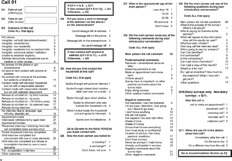
Researchers are also able to derive additional call record variables, such as number of days between calls. For face-to-face surveys, the interviewer may be asked to capture additional information about each call (e.g., if the call was made face-to-face or via a closed door/window or an intercom system), as well as additional information about the characteristics of the person talked to at the doorstep (e.g., gender, likely age, physical appearances, indicators of smoking or obesity), initial reactions of the person (e.g., type of questions asked or comments made), characteristics about the household (e.g., type of accommodation, presence of physical barriers, condition of the house, estimated value of house, likely household member composition), the immediate neighborhood (e.g., litter or graffiti present, residential or commercial area, how the interviewer feels walking alone in the area after dark). An example of a call record form for a face-to-face survey is given in Figure 12.1. We can see that the outcome of a call may distinguish many different types (Question 3). To simplify the analysis, however, survey researchers may focus on the distinction between contact/noncontact and between cooperation, refusal and other nonparticipation outcomes (for examples of such recoding see Section 12.3.2). For the purpose of nonresponse analysis, in particular if the aim is nonresponse bias correction, such paradata should be related not just to nonresponse outcomes but also to survey target variables (Little and Vartivarian, 2005; Wood and White, 2006; Kreuter et al., 2010). For example, if researchers are interested in the health status of the householder or the living conditions of children, the survey agency may aim to record information on the presence of smokers, indicators of obesity, presence of children, condition of the house and neighborhood. Such interviewer observations may be subject to measurement error and more recently, survey researchers have started to investigate the quality of such data and their potential uses for adjustments (West, 2011; Casas-Cordero and Kreuter, 2013; Sinibaldi et al., 2013).

Call record data may be recorded only once, for example, at the first visit to a household, or regularly at each call. The first type is referred to as time invariant information, the latter as time varying. Observations about persons, households and neighborhoods are referred to as interviewer observation variables and are usually recorded only once during a data collection period. (For a longitudinal survey, they may vary across waves). Time invariant information, such as interviewer observations, are usually measured at the individual or household level. Time varying information is measured at the call level (the lowest level in the hierarchy). The resulting structure of call record data can therefore be complex. For example, information may be recorded at the call level with measurements correlated across time points and at the individual and/or household level, with individuals clustered within households. For face-to-face surveys, households are usually also clustered within interviewers and areas. Sometimes such paradata are linked to other data sources, such as the survey data (either from respondents only or in case of a longitudinal study also from previous waves) but also to external sources, such as administrative or register data, Census data and information on interviewers (either available from administrative data, such as information collected routinely by the survey agency, derived information, for example based on previous interviewer performance, or from an interviewer survey), as well as area information (e.g., from administrative or Census records). Again such linked data may be available at different levels: for example, survey, administrative and interviewer observation data may be measured at the individual or household level; characteristics of the interviewer or area are measured at the interviewer and area level respectively. The complex structures of the paradata may need to be taken into account when analyzing such data.

12.3 MODELING APPROACHES

12.3.1 Analysis Approaches and the Use of Multilevel Modeling

Most of the previous work on call record data analysis focuses on the contact/ noncontact process, in particular on best times of contacting a household (Weeks et al., 1980, 1987; Kulka and Weeks, 1988; Greenberg and Stokes, 1990; Swires-Hennessy and Drake, 1992; Durrant et al., 2011; Lipps, 2012). Some work has been carried out to inform the cooperation and refusal process in surveys using call record data (Groves and Couper, 1996; Sturgis and Campanelli, 1998; Purdon et al., 1999; Sangster and Meekins, 2004; Bates et al., 2008; Durrant et al., 2013). More recent work in the area of call record and interviewer observation variables has focused on the use of such data for nonresponse adjustment which implicitly includes the specification of response propensity models (Wood and White, 2006; Peytchev and Olson, 2007; Kreuter and Kohler, 2009; Biemer et al., 2013; Kreuter et al., 2010; West, 2011).

Earlier work on call record data mostly used descriptive analysis and regression models that ignored the hierarchical structure of the data, such as the clustering of households within interviewers (Groves and Couper, 1996; Purdon et al., 1999; Sangster and Meekins, 2004; Groves and Heeringa, 2006; Bates et al., 2008) or the correlation of repeated events across calls. If multilevel models were employed mostly the final response outcome was modeled rather than the response process across calls (O’Muircheartaigh and Campanelli, 1999; Pickery et al., 2001; Durrant and Steele, 2009).

However, various sources of correlation can be identified for call record data. First, correlation may occur due to several measurements across time (i.e., here calls) and repeated outcomes per individual or household across calls. For example, a household may make several appointments or may postpone several times. The simplest way to handle repeated outcomes is to model each event separately, which may provide a workable strategy, for example, if the main interest is the outcome of one particular call only (e.g., the first call or the call at which cooperation was established). In general, however, such an approach is inefficient, since some of the factors influencing the outcome of a call may operate in the same way across all calls. In particular, results from modeling repeated events independently may be misleading, if there are unobserved characteristics that impact on the response outcomes across calls. A preferred approach is to model all such outcomes jointly. When call outcomes are repeatable, call record data have a two-level hierarchical structure with calls nested within sample units (here individuals or households). Such repeated events may then be analyzed using multilevel modeling, exhibiting a number of advantages. For example, a joint modeling approach allows the investigation of the effects of previous outcomes on the probability of later events of the same type. It also allows explicit testing whether explanatory variables that predict the occurrence of the first event also impact on subsequent events (Steele, 2005). Another common approach for the analysis of call record data is to use aggregate call data, for example, to include the total number of calls made in a model, rather than analysis across time (e.g., Bates et al., 2008). Using aggregate variables, instead of measurements across time points, however, can lead to interpretation problems, known as aggregation or ecological fallacies (Snijders and Bosker, 1999; Goldstein, 2011), since aggregate-level relationships cannot be used as estimates for corresponding lower level relationships.

Further sources of correlation may be due to the clustering of sample members within interviewers and areas. Ignoring such clustering may provide an initial working model, for example, if researchers are primarily interested in call-level influences. In general, however, such an approach will lead to underestimation of standard errors of regression coefficients, in particular of higher level variables (Snijders and Bosker, 1999; Goldstein, 2011), here of household, interviewer and area characteristics. If researchers are particularly interested in the effects of such variables single-level modeling may lead to incorrect inferences. An advantage of multilevel modeling is that it allows the incorporation of higher level (or contextual) variables into the models. In addition to such technical reasons, multilevel modeling allows the exploration of substantive questions that go beyond the scope of single-level models. For example, researchers may be particularly interested in the influence of the interviewer, for example, “how much variation is due to the interviewer as opposed to other influences?” The incorporation of a random effect to account for higher level clustering is then not a nuisance, but of substantive interest in itself.

Multilevel modeling is nowadays a standard approach for the analysis of clustered survey data and is also well established for the analysis of interviewer and area effects (Hox, 1994; O’Muircheartaigh and Campanelli, 1999; Pickery and Loosveldt, 2002, 2004; Schnell and Kreuter, 2005; Durrant and Steele, 2009; Lipps, 2009; Durrant et al., 2010). More recently, it has also been advocated for the investigation of call record data, exhibiting information at different levels and clustering of calls within higher level units (Lipps, 2009; Durrant et al., 2011, 2013). The following section presents a number of possible model specifications for the analysis of call record data and provides guidance on modeling strategy, estimation techniques and software packages. Further information on the basic ideas of multilevel modeling can be obtained from, for example, Snijders and Bosker (1999), Raudenbush and Bryk (2002), Hox (2010), Goldstein (2011), Rabe-Hesketh and Skrondal (2012). Useful online material is provided by the Centre for Multilevel Modeling (www.bristol.ac.uk/cmm). An introduction to the use of multilevel models for event history analysis can be found in Blossfeld and Rohwer (2002), Singer and Willett (2003), Steele (2005), and Goldstein (2011).

12.3.2 Specifications of Multilevel Discrete-Time Event History Models for the Analysis of Call Record Data

The particular model strongly depends on the research question and the data available. Here, different model specifications are introduced, and some of the model choices are highlighted. The methods are illustrated based on the analysis of nonresponse in surveys, modeling the process leading to a response outcome across calls (not the final response outcome). Most previous research aimed to model response at the end of the data collection process (Groves and Couper, 1998; O’Muircheartaigh and Campanelli, 1999; Durrant and Steele, 2009) and classical propensity score models of this type have been used for nonresponse adjustment (Bethlehem et al., 2011). The nonresponse process may be separated into a contact/noncontact and a cooperation/refusal stage (Groves and Couper, 1998; O’Muircheartaigh and Campanelli, 1999; Lynn and Clarke, 2002; Lynn et al., 2002; Lipps, 2009; Steele and Durrant, 2011), and this approach is employed here. Examples of interesting research questions might be “What are best times to achieve contact and/or cooperation?”, “Which type of call or calling strategy is more successful and leads more quickly to the desired response outcome?”, “Which interviewer characteristics and which doorstep approaches are more promising?”. For illustration purposes, we focus on calls within households (not within individuals), that is, on nonresponse defined at the household level. Examples from both telephone and face-to-face surveys are discussed. An additional nesting of households within interviewers is considered, which, in general, may be expected to be of greater importance for face-to-face surveys since the majority of cases are approached by the same interviewer throughout the data collection process. (This is the case for cross-sectional surveys and for one particular wave of a longitudinal survey.) When investigating several waves of a longitudinal survey interviewers may change over time and this may have implications for data analysis (see Lynn et al., 2011; Vassallo et al., 2013). For telephone surveys interviewers are randomly allocated to households and at every call a different interviewer may contact a household, leading to a potentially limited overall interviewer effect (Lynn et al., 2011; Vassallo et al., 2013), although an effect may still be expected and significant (West and Olson, 2010). Taking account of potential area effects in addition to interviewer effects, requiring a multilevel cross-classified modeling approach, is discussed elsewhere (see O’Muircheartaigh and Campanelli, 1999; Durrant et al., 2010; Goldstein, 2011; Durrant et al., 2011; Vassallo et al., 2013).

Let us define the dependent variable, , as the outcome of call t made to household i , and by interviewer j . The outcome of each call may be coded as a binary variable or as a categorical variable. Examples of a binary outcome are:

(12.1)

or

(12.2)

An example of a categorical outcome may be:

(12.3)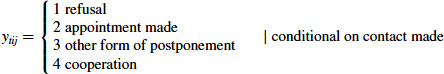

where other forms of postponement may include cancelled appointments or the interviewer withdrawing to try again later. To specify a model predicting a binary outcome as in Equations 12.1 or 12.2 a logistic model may be used. In case of a categorical outcome with more than two outcomes, a multinomial model may be estimated. Before carrying out any modeling it is advisable to explore the structure of the call record data using descriptive statistics. Researchers may investigate the possible outcomes at the first, the second, etc. call depending on different times of each call or previous call outcomes (see Weeks et al., 1987; Purdon et al., 1999; Lipps, 2009; Durrant et al., 2011, 2013). Various examples of different model specifications for the nonresponse analysis of call record data are now considered, modeling the outcome at one particular call, and across several calls for repeated and non-repeated events.

12.3.2.1 Modeling the Outcome at a Particular Call

Let us start with a simple (single-level) logistic model, modeling the binary outcome at a particular call t (time) (e.g., at the first call, , or at the call the householder cooperates or refuses) for each household i:

where is a vector of covariates with coefficients , and is the probability of the response outcome. Since we are analyzing only one particular call, the call and the household level do not need to be distinguished here. The set of covariates can contain information about the particular call (such as day and time of the call), information about the call history (if any) (e.g., total number of calls made to a household, outcome of the previous call), and covariates at the household-level to control for differences across households (e.g., single or couple households, type of accommodation, presence of children). An example of this model is discussed in Section 12.4.1 using the PASS survey data, modeling the call outcome at the first contact-call of wave 5.

Controlling in addition for the influence of the interviewer at the call, particularly important for face-to-face surveys, model (1) may be extended to a 2-level logistic model, taking account of the clustering of the call for household i within interviewer j:

where is a vector of covariates including both call and household characteristics. An advantage is that interviewer-level characteristics (e.g., years of experience, pay grade, socio-demographic characteristics, skills, attitudes, and behaviors) can now be incorporated into the model. The term is a random effect assumed to follow a normal distribution with variance , . This random effect may be used to determine, for example, how much variation in the response outcome can be attributed to the interviewer. The interpretation of the random effect is illustrated in Section 12.4.2.

12.3.2.2 Modeling the Outcome Across Calls (Discrete-Time Event History Analysis)

So far we have only introduced models that analyze the outcome at one particular call, for example, at the first call. However, researchers may be interested in analyzing the outcomes across several calls and the influence of (time varying) call-level variables. Such an approach, modeling the outcome across calls, makes use of discrete-time event history analysis (Steele et al., 1996; Singer and Willett, 2003; Steele, 2005). An advantage is that discrete-time models are essentially logistic regression models. Let us consider the example of modeling the number of calls until first contact, that is, the probability of contact at a particular call, given that no contact was made prior to that call. The first step in such an analysis is the required restructuring of the data. For the modeling of outcomes across several calls, where calls are nested within households the analysis file needs to contain a record for each call (i.e., one row in the dataset represents one call and these are nested within households). Each household may therefore contribute multiple records, up to a maximum of , with their sequence of calls terminating in first contact made or the interviewer giving up (so-called right-censored histories, i.e., the event of interest has not occurred during the considered time period).

The conditional probability of contact at call t given no contact before t—commonly referred to as the discrete-time hazard function—is defined as . The discrete-time hazard model may be written

where is a vector of covariates, with coefficients , including time-varying attributes of calls (e.g., time and day of contact attempt), (time varying) information about the call history, and time-invariant characteristics of households. The set of covariates may also include interaction terms between call-level variables and between call- and household-level characteristics, for example if researchers are interested in best times of contact for different types of households. The term is a function of the call number t, which allows the probability of contact to vary across calls (commonly referred to as the baseline logit-hazard). The form of needs to be specified by the analyst, for example by examining a plot of the hazard function (see Durrant et al., 2011). The most flexible definition is to fit as a step function, that is, where are dummy variables for calls with the maximum number of calls. In this example, since the hazard is approximately linear, a linear function is used by including the call number as an explanatory variable into the model. Groves and Heeringa (2006) provide an example of a simple application of such a time event history model analyzing cooperation versus nonparticipation. An extension of model 3 allowing for the clustering of households within interviewers, as for example the case in face-to-face surveys, is straightforward, including also a random interviewer effect . An example of such a model (i.e., of Model 3 allowing for the influence of the interviewer), is provided in Section 12.4.2, modeling time to first contact using the UK Census link study dataset. (A more comprehensive specification of this model, accounting for both interviewer and area effects, is discussed in Durrant et al. (2011)). It should be noted since the event “first contact” only occurs once to the household the model does not include a random effect for the household level (e.g., a term). We may, however, also wish to analyze repeated events occurring to a household across several calls. We now extend Model 3 to investigate such effects.

12.3.2.3 Modeling the Outcome Across Calls for Repeated Events (Discrete-Time Event History Analysis)

If response outcomes can occur several times across calls, repeated events need to be modeled. For example, the event of contact considering all calls (not just first contact) can occur more than once, and once contacted, a household may make several appointments, an interviewer may withdraw several times to come back at a later stage, or different household members may refuse to participate at different calls. A multilevel model with household random effects allows for the possibility that the events of interest may occur more than once to a household (Steele et al., 1996). For example, Chapter 7 considers best times of contact across all calls and such a model may be specified as:

where is a vector of covariates, and may include time-varying characteristics of the current call t, such as the time and day of the call, time-varying indicators of the household’s call history prior to t, and time-invariant characteristics of the household. Including interaction terms between call-level variables and household characteristics allows, for example, analysis of best times of contact for different types of households. The term is a function of the call number. Unobserved household characteristics are represented by the random effects, , assumed to follow a normal distribution.

Another example of a repeated events analysis is to model the process leading to cooperation or refusal, conditional on contact being made with a household. Model 4 may then be extended to allow for several response outcomes and, in particular for a face-to-face survey, also for the influence of the interviewer j. The dependent variable is then defined as in Section 12.3, allowing for four different response outcomes, requiring a multinomial model: refusal, appointment made, other forms of postponement (e.g., where the interviewer withdraws to come back another time or a broken appointment), and cooperation. Only contact-calls may be considered for this analysis. A multilevel multinomial logit model for the log-odds of nonparticipation outcome relative to outcome 4 (cooperation) may be written

where is a vector of covariates, including time-varying indicators of the household’s call history prior to t, characteristics of the current call such as the time and day of call t, time-invariant characteristics of the household, and potential interaction effects such as information about the interaction between householder and interviewer or interactions between call-level variables, is included as the number of the previous contact-call. Unobserved household and interviewer characteristics are represented by outcome-specific random effects, and respectively, which are each assumed to follow trivariate normal distributions to allow for potential correlation between different nonparticipation outcomes.

Applying this model to the UK Census link dataset (Section 12.4.2), Model 5 was considered in initial analysis, but due to some convergence problems in the software a slightly simplified model had to be considered. (The estimation problems of the household- and the interviewer-level variances and covariances were caused by the relatively small number of households with repeated outcomes of the same type). It was therefore decided to employ a simpler model with common, univariate random effects (, ) and outcome-specific coefficients ( and , with and fixed at 1 for identification):

where and . An example of this model is discussed in Section 12.4.2, using the UK Census link dataset. This model assumes that the odds of all nonparticipation outcomes are influenced by common sets of unmeasured household and interviewer characteristics (represented by and ), but the inclusion of and still allows their effects to differ across the three different survey outcomes (Further details of this model are provided in Durrant et al., 2013).

12.3.3 Modeling Strategy and Estimation of Models

To implement the models above in practice, it is important to consider the type of research question in mind and the type of data available. The following modeling strategy may be used: it is advisable to start with the null model not including any covariates, exploring the random effects structure, such as household and interviewer random effects. Researchers may even start with a single-level model and then enter one random effect at a time starting with the lowest level. Then, sets of covariates, one at a time, may be entered. For example, researches may first wish to control for the differences in households entering time-invariant explanatory variables before exploring the effects of time varying variables on the outcome of interest. Higher level variables, such as information on interviewers, may then be entered, for example, to see how much of the interviewer variation can be explained.

Different types of software may be used for the different models. The simple logistic regression model (Model 2) can be fitted using any standard software (e.g., SPSS, STATA, Splus, SAS). Multilevel logistic models can be fitted using either dedicated software for modeling multilevel models, such as MLwiN (see Browne, 2009; Rasbash et al., 2009), or, for example a specified function in a statistical package such as STATA (e.g., command “xtlogit”) (see Rabe-Hesketh and Skrondal, 2012). Depending on the software, different estimation methods may be available. For example, MLwiN offers both quasi-likelihood and Markov chain Monte Carlo (MCMC) estimation (Browne, 2009). STATA uses numerical quadrature. Overall, the MCMC option in MLwiN may provide the most flexible approach, and has been shown to produce improved estimates over quasi-likelihood methods in terms of unbiasedness (Browne and Draper, 2006). It also offers advantages in terms of running time for some types of models. Model 5′ can only be fitted in the software package aML based on maximum likelihood estimation (Lillard and Panis, 2003). The use of all three software packages (MLwiN, STATA and aML) are illustrated in the examples in Section 12.4. Reviews of software packages for modeling multilevel data can be obtained from the Centre for Multilevel Modeling website (www.bristol.ac.uk/cmm/learning/mmsoftware).

Evaluation of model fit and model complexity depends on the estimation method used. For example, a likelihood ratio test may be employed for maximum likelihood estimation procedures and the Deviance Information Criterion (DIC; (Spiegelhalter et al., 2002) for MCMC estimation, a Bayesian analogue of the likelihood-based Akaike information criterion which balances model fit and model complexity, where models with a smaller DIC indicate a better fit). One potential difficulty when using discrete-time event history analysis may be that the required restructuring of the data leads to an increase in the size of the dataset which in turn can lead to longer computation times for more complex models with random effects.

12.4 ILLUSTRATION OF CALL RECORD DATA ANALYSIS USING TWO EXAMPLE DATASETS

12.4.1 Analyzing Call Outcomes in the PASS Longitudinal Survey

12.4.1.1 Data and Methods

The PASS survey is a longitudinal household study for labor market, welfare state, and poverty research in Germany. Data have been collected annually since 2006/2007, applying a mixed-mode design of computer-assisted telephone interviewing (CATI) and computer-assisted personal interviewing (CAPI). PASS administers a household-level questionnaire to be answered by the head of household as well as a person-level questionnaire for each household member aged 15 years and older. The PASS survey collects detailed call record data at every wave, including for example time and day of each call, the outcome of the call, the mode, whether a call was a regular or a refusal conversion call, or part of the Turkish or Russian language field work and indicators of the various samples (population and recipient samples, refreshment samples). An advantage of the study is that household- and person-level survey information from all previous waves are available including also interviewer identifiers that enable linkage to information on interviewers. Further information on the survey sampling design, core questionnaire modules and data structure are provided in Schnell (2007), Rudolph and Trappmann (2007), Trappmann et al. (2010), and the PASS user guide (Bethmann and Gebhardt, 2011).

In this first example, we are interested in the probability of household cooperation at the first contact call. In particular, we aim to identify best calling times to achieve cooperation, taking account of previous wave call data, some aspects of the survey design and a vector of household- and person-level covariates. The research may inform survey practitioners on best calling strategies not just to achieve contact but in particular (immediate) cooperation and may inform about the usefulness of previous call data information. In the first instance, a simple logistic regression model is employed in line with Model 1, modeling the binary outcome of interest (household cooperation) at one particular call, here the first contact call, for each household. Call record data from the fifth wave of the telephone component is used, linked to call record data from the previous wave and to household and personal-level survey information, also from the previous wave, providing information on both respondents and nonrespondents to wave 5. The analysis sample consists of 4417 first contact-calls, that is, one call per household. Households that were never contacted are excluded from the analysis. The sample is further restricted to panel households that all have participated in the previous wave. For the analysis of best calling times we restrict the analysis sample to the telephone component since the automatic dialing routines in the centralized CATI facility ensure a quasi-random allocation of calls (and calling times) of interviewers to sample cases.

12.4.1.2 Results of Logistic Regression Model: Cooperation at First Contact

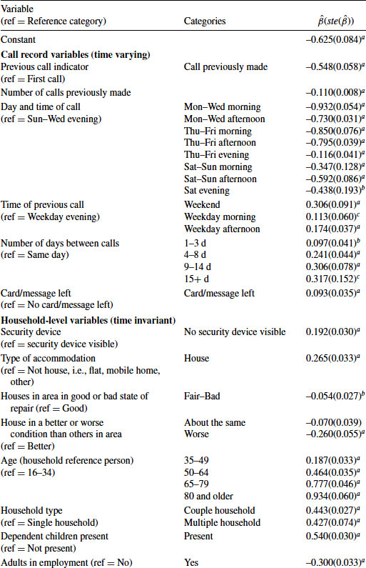
Table 12.1 presents estimated coefficients of the logistic regression model. The selection of demographic and socio-economic variables resembles covariates regularly included in models of panel attrition that aim to detect differential response propensities of relevant subgroups (Watson and Wooden, 2009; Uhrig, 2008; Kroh, 2010). The key findings are as follows:

Table 12.1 Estimated Coefficients (and Standard Errors) for Logistic Regression Model for Cooperation at First Contact (Model 1) Using the PASS Survey

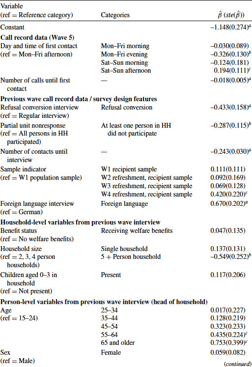
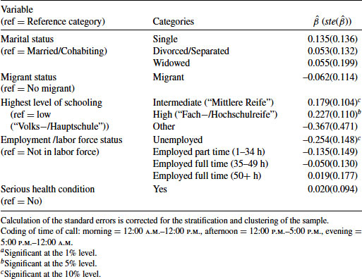
Compared to the reference time window, weekday evenings do not appear to be well suited to gain immediate cooperation. This can be shown to hold rather uniformly across all weekday evenings (based on additional analyses not presented here). There is also some evidence that weekend afternoons may be more suitable to achieve immediate cooperation, although the coefficient for that time window is only marginally significant. Again, based on more detailed analyses not shown here, this effect appears to be driven mainly by higher cooperation rates on Saturday afternoons, with immediate cooperation on Sunday afternoons being little different from weekday afternoons. In addition, the number of calls until first contact (i.e., previous noncontact calls) is predictive of immediate household cooperation. That is, sample cases that are difficult to reach also tend to be those that do not participate once successfully contacted, at least not at the first contact call. Using information generated from previous wave call data, we can see that all indicators for respondents’ willingness (or reluctance) to cooperate at the previous wave are highly predictive of current wave (non-) cooperation. For example, if the previous interview could be obtained only after refusal conversion efforts and, if one or more eligible household members did not give their person-level interview, then household cooperation at the current wave is much lower. The single strongest predictor of current wave non-cooperation at first contact is the number of contacts that were necessary to obtain the interview in the previous wave. With regard to the household and person characteristics, included as controls, we can see, for example, that immediate cooperation tends to be higher in smaller households (<5 household members), with a reference person aged 55+ years, with an intermediate to high level of schooling, and where the head of household is currently not unemployed. Overall, we find that most of the demographic and socio-economic variables were only weakly predictive of the cooperation decision, if at all.

The research findings may inform survey practitioners on how best to achieve (immediate) cooperation at a call without the need for follow-up calls, reducing effort and costs. In particular, the results show that previous call record information is indeed beneficial in predicting the outcome at the next wave. Further research is needed to investigate the usefulness of previous call record data to inform best calling strategies for particular cases.

When interpreting these findings, we should bear in mind that we are considering results for cooperation at one particular call only, here the first contact call. For cooperation at second, third, and higher contact calls, different relationships with the explanatory variables may hold. So far, we have looked at cooperation as a binary outcome, implicitly comparing cooperation to all other possible outcomes. Some of these outcomes, such as obtaining an appointment at first contact, may actually be quite favorable in terms of the final outcome. Further examples will now extend this type of analysis, investigating outcomes across all calls and allowing for a range of response outcomes at each call.

12.4.2 Analyzing Call Outcomes in the UK Census Nonresponse Link Study

12.4.2.1 Data and Methods

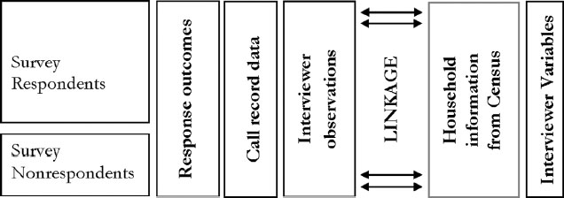
The UK Census link study is a rich dataset that links paradata of six UK face-to-face cross-sectional household surveys to UK Census records and information on interviewers, as illustrated in Figure 12.2. An advantage is that information on both responding and nonresponding households is available. The paradata contains detailed call record data, including the household response outcome, and interviewer observation variables. Two multilevel discrete-time event history models are fitted to the data modeling the outcome across calls. First, Model 3 is employed to analyze the number of calls until first contact controlling for interviewer effects. Of interest are, for example, best times of contact (also for different household types), and the influence of the interviewer and interviewer strategies on the contact process. The analysis sample contains 37,879 calls (only including calls until first contact or until the household was coded as a noncontact), 16,700 households (of which 1017 households were never contacted), nested within 565 interviewers.

In the second application, Model 5 (due to some convergence problems model 5′) is fitted to investigate the process leading to cooperation or refusal. Survey researchers might be interested in best times of persuading sample members to cooperate, effectiveness of interviewer doorstep approaches and the influence of the interviewer on the cooperation process. The analysis sample includes 38,816 contact-calls, nested within 15,782 households and 565 interviewers. It should be noted, since the data does not come from a controlled experiment but reflect observational data, causal effects cannot be inferred. (For further information on the specifics of the dataset see White et al. (2001); Freeth et al. (2002); Beerten and Freeth (2004). Comprehensive model interpretations can be found in Durrant et al. (2011, 2013) respectively).

12.4.2.2 Results of Discrete-Time Event History Model: Probability of First Contact

Table 12.2 presents the modeling results for the contact analysis. The model includes a range of household-level variables, from both interviewer observations and Census records, to control for differences across households. For example, we may expect, and this is shown in the model, that the probability of contact depends on physical impediments to the household, accommodation type, number of people in the household, employment status of household members and the presence of children. The influence of the time varying call record variables may be summarized as follows: The probability of contact is highest for the first call and decreases thereafter. The highly significant and negative coefficient on “number of previous calls” indicates that the decrease in the odds of contact is about 10% for each additional call net of all other variables in the model (10%=([1−exp(−0.110)]*100). We tested interaction effects between number of previous calls with all other variables in the model to investigate potential non-proportional effects of covariates, but did not find evidence that the effect of any variable differed across calls. On average, best times to contact a household are evening and weekend calls, confirming results from previous research (Weeks et al., 1980; Purdon et al., 1999). To investigate best contacting times for each type of household interaction effects between the time of the contact and household characteristics can be incorporated and this was carried out in Durrant et al. (2011), deriving predicted probabilities for different contact times and types of households. If the previous call was already on a weekday evening then establishing contact at the next call becomes increasingly less likely, indicating a potentially more difficult to contact household. The time of the previous call may be interacted with the time of the current call to inform survey agencies of best calling times depending on the call history. The effect of the number of days between calls suggests that leaving a few days between calls, ideally about 1 or 2 weeks, increases the probability of contact compared to returning on the same day. The model also indicates an increase in the probability of contact at the next call if a card or message was left, providing some support for this to be a good interviewer contacting strategy.

Table 12.2 Estimated Coefficients (and Standard Errors) for 2-Level Discrete-Time Event History Model, Modeling the Number of Calls Until First Contact (Model 3) and Allowing for Interviewer Effects (Using the Census Link Study Dataset)

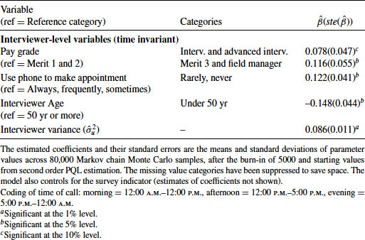
The significant interviewer variance () indicates variation between interviewers in their contact rates. Interpreting as the effect of a one standard deviation increase in the unobserved characteristics represented by the random interviewer effect we find that, after adjusting for covariates in the model, an interviewer whose unobserved characteristics place them at one standard deviation above the average has a 34% higher odds of making contact than an “average” interviewer. The inclusion of the interviewer characteristics reduces the between-interviewer variance from 0.11 for a model without these characteristics (results not shown) to 0.086 (for model in Table 12.2), explaining about 22% of the interviewer variance. The inclusion of interviewer-level variables helps to identify interviewer characteristics that may impact positively on the probability of contacting a household. Interviewers in higher pay grades (reflecting more experienced and more skillful interviewers) and older interviewers (above the age of 50 years) are more likely to establish contact. The latter effect may be explained by the potentially higher experience of older interviewers, they may appear more trustworthy or they may have fewer time-constraining commitments outside their job, such as looking after young children, allowing greater flexibility on calling times. Survey agencies are particularly interested in behavioral differences between interviewers and the influence of interviewer strategies on the probability of contact is therefore also explored. For example, interviewers, who always or frequently use the phone to establish contact, rather than visiting the household in person, perform worse than interviewers who rarely or never use the phone. This may be an indicator of interviewer effort, with interviewers putting in more effort and dedicating more time to each sample unit being more successful.

12.4.2.3 Results of Discrete-Time Event History Model (Repeated Events): Modeling the Probability of Cooperation or Refusal

The results of Model 5′, predicting possible response outcomes at the contact stage, are presented in Tables 12.3 and 12.4. The model includes time varying variables describing characteristics of the current call, controlling for the call history and a range of household characteristics (Table 12.3). We can see that with each additional contact refusals, appointments and postponements are less likely to occur (although the effect is not significant for refusal in the particular model here), possibly indicating that staying in contact with a household may impact positively on participation. On the other hand, the larger the number of intermediate noncontact calls, the lower is the likelihood of participation at the next call. Having made an appointment at the previous call, the current call is much less likely to result in refusal, postponement or another appointment, increasing the chances of cooperation. Good times to call to achieve cooperation are afternoons, with the lowest probabilities for evening calls, also supporting findings from the PASS analysis in Section 12.4.1. This result indicates that best times to establish cooperation may not be best times to establish contact (i.e., evenings and weekends). Evening calls, however, may still be necessary, if contact was not established at other times, and may be used to make an appointment—a strategy often adhered to by interviewers. The initial reaction from the householder at the doorstep is found to be a good indicator of cooperation. If, for example, the householder makes a negative comment or does not ask any questions the likelihood for all nonparticipation outcomes is significantly increased. Survey agencies may use the initial responses, such as a household making a negative comment, as an early indication for a more difficult case requiring potentially a revised contacting strategy, for example, sending a different interviewer or offering a higher incentive. Characteristics of the person talked to at the doorstep may also provide clues on likely participation rates and may inform possible contacting strategies at the next call. For example, younger householders are more likely to refuse, make an appointment for another time, or to postpone. Women are more likely to make appointments or to postpone.

Table 12.3 Estimated Coefficients (and Standard Errors) of Multilevel Multinomial Discrete-Time Event History Model for Cooperation Controlling for Household and Interviewer Characteristics (Model 5′)

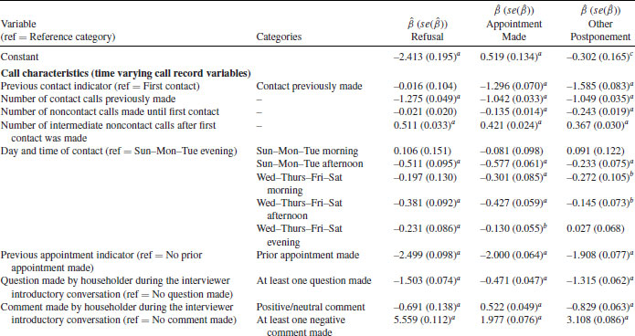
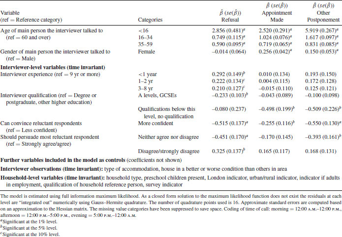
Table 12.4 Estimated Household and Interviewer Random Effect Parameters from the Multilevel Multinomial Logistic Discrete-Time Event History Model (Standard Errors in Parentheses) for Cooperation Across Controlling for Household and Interviewer Characteristics (Model 5′)

Parameter	Estimate (Standard Error)
Household common standard deviation	1.696 (0.091)a
Household random effect loadings
Refusal
Appointment made	0.857 (0.045)a
Other postponement	1.321 (0.063)a
Interviewer common standard deviation	0.699 (0.039)a
aSignificantly different from zero at the 1% level. bConstrained to equal 1.

Table 12.4 indicates significant household-level variation () due to unmeasured household characteristics, with evidence of differential household effects across the three nonparticipation outcomes (using a t-test the coefficients and on the household random effects are not equal to 1), with a stronger household effect for postponement and a weaker effect for appointments. We find significant between-interviewer variation (), indicating that interviewers have indeed a significant influence on response outcomes at a particular call. There was no evidence to suggest differential interviewer effects across the different nonparticipation outcomes (based on a likelihood ratio test the coefficients () on the interviewer random effects are assumed to be equal to 1), which implies that unmeasured interviewer characteristics have the same effect on the log-odds of each of the three nonparticipation outcomes. (For further details on the random effects interpretation see Durrant et al., 2013). Interviewer-level variables are entered into the model to explain part of the interviewer-level random effect. For example, as one may expect, interviewers with less than 1 year experience have higher refusal rates Table 12.3. Evidence for the importance of the attitude of interviewers is found. Interviewers that are more confident in their ability to convince reluctant respondents have significantly less refusals, appointments and postponements. Interviewers that disagree that they should persuade reluctant respondents are significantly more likely to experience a refusal. Models of this type may inform improvements to interviewer calling strategies, interviewer training and evaluation of interviewer performance. For example, interviewers may be trained to pick up important clues about the characteristics of the household or the future response behavior early on and to feed these back to field management. Areas may be identified where interviewers may be better trained in responding to initial reactions of the householder on the doorstep.

12.5 SUMMARY

This Chapter aimed to provide an overview over different modeling approaches for the analysis of call record data. Examples of research questions and available data in the context of nonresponse in both telephone and face-to-face surveys were discussed. Some considerations were given to cross-sectional and longitudinal surveys. The models presented allowed for the clustering of outcomes across calls and extensions incorporating the nesting of sample members within interviewers were considered, using multilevel discrete-time event history analysis. The models may inform effective and efficient interviewer calling strategies. They may provide guidance to survey practitioners on how to model call record data and to identify important factors influencing the nonresponse process. For example, researchers may aim to analyze best times of contact, also for particular type of sample members, best interviewer calling strategies at the doorstep and variations across interviewers. The results indicate that time-varying call record information, such as characteristics of the current call and the call history, play an important role in predicting the outcome of a call. The models may be used in responsive and adaptive survey designs to inform intervention decisions and best calling times and strategies.

ACKNOWLEDGMENTS

The research was funded by the UK Economic and Social Research Council (ESRC), “The Use of Paradata in Cross-Sectional and Longitudinal Surveys,” grant number: RES-062-23-2997. This work contains statistical data from ONS which is Crown copyright and reproduced with the permission of the controller of HMSO and Queen’s Printer for Scotland. The use of the ONS statistical data in this work does not imply the endorsement of the ONS in relation to the interpretation or analysis of the statistical data. This work uses research datasets which may not exactly reproduce National Statistics aggregates. This study uses the factually anonymous data of the PASS. Data access was provided via a Scientific Use File supplied by the Research Data Centre (FDZ) of the German Federal Employment Agency (BA) at the Institute for Employment Research (IAB).

REFERENCES

Baruch, Y. and Holtom, B. (2008). Survey Response Rate Levels and Trends in Organizational Research. Human Relations, 61(8):1139–1160.

Bates, N., Dahlhamer, J., and Singer, E. (2008). Privacy Concerns, Too Busy, or Just Not Interested: Using Doorstep Concerns to Predict Survey Nonresponse. Journal of Official Statistics, 24(4):591–612.

Beerten, R. and Freeth, S. (2004). Exploring Survey Nonresponse in the UK: the Census-Survey Nonresponse Link Study. Technical report, Office for National Statistics, Working Paper, London.

Bethlehem, J., Cobben, F., and Schouten, B. (2011). Handbook in Nonresponse in Household Surveys. Wiley and Sons, Inc.

Bethmann, A. and Gebhardt, D. (2011). User guide “Panel Study Labour Market and Social Security” (PASS), wave 3. FDZ-Datenreport 04/2011.

Biemer, P., Chen, P., and Wang, K. (2013). Using Level-of-Effort Paradata in Non-Response Adjustments with Application to Field Surveys. Journal of the Royal Statistical Society, Series A (Statistics in Society), Special issue on The Use of Paradata in Social Survey Research, 176(1):147–168.

Blom, A., Jackle, A., and Lynn, P. (2010). The Use of Contact Data in Understanding Cross-national Differences in Unit Nonresponse. In Harkness J.A., Braun M., Edwards B., Johnson T.P., Lyberg L.E., Mohler P.Ph., Pennell B.-E., Smith T.W., editors, Survey Methods in Multinational, Multiregional, and Multicultural Contexts, pages 335–354. Wiley and Sons, Inc., Hoboken, NJ.

Blossfeld, H. and Rohwer, G. (2002). Techniques in Event History Modeling: New Approaches to Casual Analysis. 2nd edition, Taylor and Francis.

Browne, W. (2009). MCMC Estimation in MLwiN v2.1. Centre for Multilevel Modeling.

Browne, W. and Draper, D. (2006). A Comparison of Bayesian and Likelihood-based Methods for Fitting Multilevel Models. Bayesian Analysis, 1:473–550.

Casas-Cordero, C., Kreuter, F., Wang Y., and Babey, S. (2013). Assessing the Measurement Error Properties of Interviewer Observations of Neighbourhood Characteristics, Journal of the Royal Statistical Society, Series A, Special issue on The Use of Paradata in Social Survey Research, 176(1):227–249.

Conrad, F.G., Broome, J.S., Benkí, J.R., Kreuter, F., Groves, R.M., Vannette, D., and McClain, C. (2013). Interviewer Speech and the Success of Survey Invitations, Journal of the Royal Statistical Society, Series A, Special issue on The Use of Paradata in Social Survey Research, 176(1):191–210.

Durrant, G., D’Arrigo, J., and Steele, F. (2011). Using Field Process Data to Predict Best Times of Contact Conditioning on Household and Interviewer Influences. Journal of the Royal Statistical Society, Series A, 174(4):1029–1049.

Durrant, G.B., D'Arrigo, J., and Steele, F. (2013). Analysing Interviewer Call Record Data by Using a Multilevel Discrete-Time Event History Modelling Approach, Journal of the Royal Statistical Society, Series A, Special issue on The Use of Paradata in Social Survey Research, 176(1): 251–269.

Durrant, G. and Steele, F. (2009). Multilevel Modelling of Refusal and Non-contact in Household Surveys: Evidence from Six UK Government Surveys. Journal of the Royal Statistical Society, Series A, 172(2):361–381.

Durrant, G.B., Groves, R.M., Staetsky, L., and Steele, F. (2010). Effects of Interviewer Attitudes and Behaviors on Refusal in Household Surveys. Public Opinion Quarterly, 74(1):1–36.

Freeth, S., Kane, C., and Cowie, A. (2002). Survey Interviewer Attitudes and Demographic Profile, Preliminary Results from the 2001 ONS Interviewer Attitudes Survey. Paper presented at the Government Statistical Service Methodology Conference London, July 8, 2002.

Goldstein, H. (2011). Multilevel Statistical Models. 4th edition, Wiley and Sons, Inc.

Greenberg, B. and Stokes, S. (1990). Developing an Optimal Call Scheduling Strategy for a Telephone Survey. Journal of Official Statistics, 6(4):421–435.

Groves, R.M. and Couper, M.P. (1996). Contact-Level Influences on Cooperation in Face-to-Face Surveys. Journal of Official Statistics, 12(1):63–83.

Groves, R.M. and Couper, M.P. (1998). Nonresponse in Household Interview Surveys. Wiley and Sons, Inc., New York.

Groves, R.M. and Heeringa, S.G. (2006). Responsive Design for Household Surveys: Tools for Actively Controlling Survey Nonresponse and Costs. Journal of the Royal Statistical Society, Series A: Statistics in Society, 169(3):439–457.

Hox, J. (1994). Hierarchical Regression Models for Interviewer and Respondent Effects. Sociological Methods and Research, 22(3):300–318.

Hox, J. (2010). Multilevel Analysis: Techniques and Applications. Quantitative Methodology Series.

Kreuter, F. and Kohler, U. (2009). Analyzing Contact Sequences in Call Record Data. Potential and Limitations of Sequence Indicators for Nonresponse Adjustments in the European Social Survey. Journal of Official Statistics, 25(2):203–226.

Kreuter, F., Olson, K., Wagner, J., Yan, T., Ezzati-Rice, T., Casas-Cordero, C., Lemay, M., Peytchev, A., Groves, R., and Raghunathan, T. (2010). Using Proxy Measures and other Correlates of Survey Outcomes to Adjust for Non-response: Examples from Multiple Surveys. Journal Of The Royal Statistical Society, Series A, 173(2):389–407.

Kroh, M. (2010). Documentation of Sample Sizes and Panel Attrition in the German Socio-Economic Panel (SOEP) (1984 until 2009). Data Documentation 50.

Kulka, R. and Weeks, M. (1988). Toward the Development of Optimal Calling Protocols for Telephone Surveys: A Conditional Probabilities Approach. Journal of Official Statistics, 4(4):319–332.

Laflamme, F., Maydan, M., and Miller, A. (2008). Using Paradata to Actively Manage the Survey Data Collection Process. Proceedings of the Survey Research Methods Section, American Statistical Association, pages 630–637.

Lee, S., Brown, E., Grant, D., Belin, T., and Brick, J. (2009). Exploring Nonresponse Bias in a Health Survey Using Neighborhood Characteristics. American Journal of Public Health, 99(10):1811–1817.

Lillard, L. and Panis, C. (2003). aML Multilevel Multiprocess Statistical Software, Version 2.0. EconWare.

Lipps, O. (2009). Cooperation in Centralised CATI Household Panel Surveys—A Contact-based Multilevel Analysis to Examine Interviewer, Respondent, and Fieldwork Process Effects. Journal of Official Statistics, 25(3):323–338.

Lipps, O. (2012). A Note on Improving Contact Times in Panel Surveys. Field Methods, 24(1):95–111.

Little, R.J.A. and Vartivarian, S. (2005). Does Weighting for Nonresponse Increase the Variance of Survey Means? Survey Methodology, 31(2):161–168.

Lynn, P. and Clarke, P. (2002). Separating Refusal Bias and Non-contact Bias: Evidence from UK National Surveys. Statistician, 51:319–333.

Lynn, P., Clarke, P., Martin, J., and Sturgis, P. (2002). The Effects of Extended Interviewer Efforts on Nonresponse Bias. In Groves, R., Dillman, D., Eltinge, J., and Little, R., editors, Survey Nonresponse, pages 135–147. Wiley and Sons, Inc., New York.

Lynn, P., Kaminska, O., and Goldstein, H. (2011). Panel Attrition: How Important is it to Keep the Same Interviewer? ISER Working paper Series.

Maynard, D. and Schaeffer, N. (1997). Keeping the Gate: Declinations of the Request to Participate in a Telephone Survey Interview. Sociological Methods and Research, 26:34–79.

O’Muircheartaigh, C. and Campanelli, P. (1999). A Multilevel Exploration of the Role of Interviewers in Survey Non-response. Journal of the Royal Statistical Society, Series A, 162(3):437–446.

Peytchev, A. and Olson, K. (2007). Using Interviewer Observations to Improve Nonresponse Adjustments: NES 2004. Proceedings of the Survey Research Methods Section, American Statistical Association, pages 3364–3371.

Pickery, J. and Loosveldt, G. (2002). A Multilevel Multinomial Analysis of Interviewer Effects on Various Components of Unit Nonresponse. Quality and Quantity, 36(4):427–437.

Pickery, J. and Loosveldt, G. (2004). A Simultaneous Analysis of Interviewer Effects on Various Data Quality Indicators with Identification of Exceptional Interviewers. Journal of Official Statistics, 20(1):77–89.

Pickery, J., Loosveldt, G., and Carton, A. (2001). The Effects of Interviewer and Respondent Characteristics on Response Behavior in Panel Surveys. Sociological Methods and Research, 29(4):509–523.

Purdon, S., Campanelli, P., and Sturgis, P. (1999). Interviewers Calling Strategies on Face- to- Face Interview Surveys. Journal of Official Statistics, 15(2):199–216.

Rabe-Hesketh, S. and Skrondal, A. (2012). Multilevel and Longitudinal Modeling using Stata, Volume I and II. Stata Press, College Station, 3rd edition, Texas.

Rasbash, J., Steele, F., Browne, W., and Goldstein, H. (2009). A User’s Guide to MLwiN v2.1. Centre for Multilevel Modeling.

Raudenbush, S.W. and Bryk, A. (2002). Hierarchical Linear Models: Applications and Data Analysis Methods. 2nd edition. Sage Publications. Newbury Park, CA.

Rudolph, H. and Trappmann, M. (2007). Design und Stichprobe des Panels, Arbeitmarkt und Soziale Sicherung (PASS). In Promberger, M., editor, Neue Daten für die Sozialforschung. IAB Nürnberg.

Sangster, R. and Meekins, B. (2004). Modeling the Likelihood of Interviews and Refusals: Using Call History Data to Improve Efficiency of Effort in a National RDD Survey. In Proceedings of the Section on Survey Research Methods of the American Statistical Association. http://www.bls.gov/osmr/abstract/st/st040090.htm.

Schnell, R. (2007). Alternative Verfahren zur Stichprobengewinnung für ein Haushaltspanelsurvey mit Schwerpunkt im Niedrigeinkommens- und Transferleistungsbezug; In Promberger, M., editor, Neue Daten für die Sozialstaatsforschung: Zur Konzeption der IAB-Panelerhebung “Arbeitsmarkt und Soziale Sicherung.” IAB, Nürnberg. pages 33–59.

Schnell, R. and Kreuter, F. (2005). Separating Interviewer and Sampling-Point Effects. Journal of Official Statistics, 21(3):389–410.

Singer, J. and Willett, J. (2003). Applied Longitudinal Data Analysis: Modeling Change and Event Occurrence. Oxford University Press.

Sinibaldi, J., Durrant, G.B., and Kreuter, F. (2013). Evaluating the Measurement Error of Interviewer Observed Paradata, Public Opinion Quarterly, Special issue: Topics in Survey Measurement and Public Opinion, 77(1):173–193.

Snijders, T. and Bosker, R. (1999). Multilevel Analysis. An Introduction to Basic and Advanced Multilevel Modeling. Sage Publications, Thousand Oaks, CA.

Spiegelhalter, D.J., Best, N., Carlin, B., and van der Linde, A. (2002). Bayesian Measures of Model Complexity and Fit (with Discussion). Journal of the Royal Statistical Society, Series B, 64:583–639.

Steele, F. (2005). Event History Analysis. NCRM Methods Review Papers, NCRM/004.

Steele, F., Diamond, I., and Amin, S. (1996). Immunization Uptake in Rural Bangladesh: a Multilevel Analysis. Journal of the Royal Statistical Society, Series A, 159:289–229.

Steele, F. and Durrant, G. (2011). Alternative Approaches to Multilevel Modeling of Survey Noncontact and Refusal. International Statistical Review, 79(1):70–91.

Sturgis, P. and Campanelli, P. (1998). The Scope for Reducing Refusals in Household Surveys: An Investigation based on Transcripts of Tape-recorded Doorstep Interactions. Journal of the Market Research Society, 40(2):121–139.

Swires-Hennessy, E. and Drake, M. (1992). The Optimum Time at which to Conduct Interviews. Journal of the Market Research Society, 34(1):61–72.

Trappmann, M., Gundert, S., Wenzig, C., and Gebhardt, D. (2010). PASS—A Household Panel Survey for Research on Unemployment and Poverty. Schmollers Jahrbuch (Journal of Applied Social Science Studies), 130(4):609–622.

Uhrig, N.S. (2008). The Nature and Causes of Attrition in the British Household Panel Survey. ISER Discussion, (5).

Vassallo, R, Durrant, G.B., Smith, P., and Goldstein, H. (2013). Interviewer Effects on Nonresponse Propensity in Longitudinal Surveys: A Multilevel Modeling Approach, under review.

Watson, N. and Wooden, M. (2009). Identifying Factors Affecting Longitudinal Survey Response. In Lynn, P., editor, Methodology of Longitudinal Surveys, pages 157–181. Wiley and Sons, Inc., Chichester.

Weeks, M.F., Kulka, R., and Pierson, S. (1987). Optimal Call Scheduling For A Telephone Survey. Public Opinion Quarterly, 51(4):540–549.

Weeks, M.F., Jones, B.L., Folsom, R.E., and Jr. Benrud, C.H. (1980). Optimal Times to Contact Sample Households. Public Opinion Quarterly, 44(1):101–114.

West, B.T. (2011). Measurement Error in Survey Paradata. Proceedings of the Survey Research Methods Section, American Statistical Association.

West, B.T. and Olson, K. (2010). How much of Interviewer Variance is Really Nonresponse Error Variance? Public Opinion Quarterly, 74(5):1004–1026.

White, A., Freeth, S., and Martin, J. (2001). Evaluation of Survey Data Quality using Matched Census-Survey Records. Paper presented at the International Conference on Quality in Official Statistics.

Wood, A.M., White, I.R., and Hotopf, M. (2006). Using Number of Failed Contact Attempts to Adjust for Non-ignorable Non-response. Journal of the Royal Statistical Society, Series A: Statistics in Society, 169(3):525–542.