
CHAPTER 6
DESIGN AND MANAGEMENT STRATEGIES FOR PARADATA-DRIVEN RESPONSIVE DESIGN: ILLUSTRATIONS FROM THE 2006--2010 NATIONAL SURVEY OF FAMILY GROWTH
6.1 INTRODUCTION
Survey design requirements have increased substantially over the last several decades. Today, scientists and policy makers require more extensive measures on larger samples, and to collect those measures on a more frequent basis from more specific segments of a population in greater geographic and demographic detail than ever before. At the same time, survey researchers have found that the environment for conducting surveys is one of increasing uncertainty regarding successful implementation.
Surveys on families and family growth, for example, clearly show the increasing demands, and uncertainties, of survey research. Family growth surveys have been conducted in the United States since 1955. The first such survey was conducted over the course of several months using paper and pencil methods and a population of Caucasian women aged 18--39 years who were currently married (Mosher and Bachrach, 1996). The most recently completed survey in the subsequent U.S. fertility survey series, the 2006–2010 National Survey of Family Growth (NSFG), obtained interviews from women and men 15--44 years of age regardless of race, ethnicity, or marital status (Groves et al., 2009). The 2006–2010 interviews were conducted in a continuous sequence of 16 national samples using computer-assisted personal interviews (CAPI) and self-administered systems, and had a sample size seven times larger than the 1955 survey.
With increased complexity and size comes increased cost and a search for more efficient data collection methods that either maintain or improve survey data quality. The science of survey methodology is deeply engaged in these issues, continually experimenting with new strategies and approaches to create more and better quality data with less effort and lower costs. Gains in efficiency and data quality are apparent. For example, in the NSFG series, Cycle 6 conducted in 2002–2003 produced roughly 12,500 completed interviews with women and men nationwide (Groves et al., 2004). Interviews were 60–80 min conducted using a CAPI questionnaire containing questions on sexual and fertility experiences of the respondent. More sensitive items (e.g., risk behaviors for HIV) were administered using audio computer-assisted self-interview (ACASI). Using a new design for 2006–2010 data collection, NSFG produced approximately 22,500 interviews 60–70 min in length and using the same computer-assisted data collection modes for approximately the same cost (Groves et al., 2009).
This striking increase in number of completed interviews was achieved through a number of methodological and operational advances. One key advance was an extensive use of paradata exploited via a new generation of design and management tools. A second advance was the conceptualization and implementation of design features that attempted to respond to survey conditions in real time, the so-called responsive designs (Groves and Heeringa, 2006). This advance used information about data collection field work to alter field and sampling protocols during survey data collection to achieve greater efficiency and improvements in data quality. A third key advance in the NSFG series was the use of web-based centralized management systems that built on previous investment and transition to computer-assisted interviewing (CAI). These systems added to the ability to collect, transmit, and analyze paradata during survey operations.
We examine in this chapter how these three advances were implemented in the 2006–2010 NSFG. The examination provides insights into the micro-dynamics of social data collection, showing how the advances facilitated interventions that increased efficiency and data quality. It also shows how the use of paradata for responsive design altered, in real time, the management of a large-scale continuous survey operation to improve survey outcomes. There are important lessons for all types of surveys as the techniques discussed here are translated into specific design features and strategies.
6.2 FROM REPEATED CROSS-SECTION TO CONTINUOUS DESIGN
In order to understand the design transformation in the NSFG, one must understand the NSFG Cycle 6 (2002–2003) design. Cycle 6 was conducted by the National Center for Health Statistics (NCHS). It collected data on pregnancy, childbearing, men and women’s health, and parenting from a national sample of women and men 15–44 years of age in the United States. The survey was based on a national stratified multistage probability sample, and was the first NSFG to include a sample of men. In addition, the sample oversampled Hispanic and African-American subgroups and teenagers 15–19 years of age. These oversamples were designed to provide a sufficient number of completed interviews for these groups in subsequent analysis (Lepkowski et al., 2006).
Field work was carried out by the University of Michigan's Institute for Social Research (ISR) under a contract with NCHS. More than 250 female interviewers conducted in-person, face-to-face interviews using laptop computers, including an ACASI portion of the interview in which the respondent read or listened to questions and entered responses directly into the laptop.
The sample units at the first and subsequent stages of selection were divided into replicate samples to facilitate management. Since it was not possible to train all interviewers at one time, sample releases corresponded to the completion of three interviewer training sessions. Each release was a replicate of the overall sample design.
Interviewers were responsible for collecting and uploading data throughout the 11-month study period as interviews were completed. Their work assignments included cases that needed to be screened to determine whether anyone 15–44 years of age resided at the address (the screener cases), selection for interview of one eligible person from each household with eligible persons, and interviewing sample persons selected for the interview (the main cases). They also collected and uploaded observations about contacts with sample households, about the persons in the sample and their households, and about the neighborhoods. Interviewers were supervised by a large staff of team leaders and supervisors divided into regional staff.
Data collection was halted after 10 months and a sample was selected of remaining incomplete, or nonresponding, addresses. A selection was also made of interviewers to continue work in the eleventh month, a second phase of data collection. Second phase interviewers had a considerably reduced number of addresses to contact and interview. In all, across the three releases and two phases of data collection, 12,571 interviews—7643 females and 4928 males—were completed, the largest NSFG sample to that date.
By 2006, when the NSFG was to be repeated, NCHS faced rising labor costs and a population increasingly difficult to contact and reluctant to participate. Substantially increased costs of data collection were anticipated.
Following the completion of the 2002–2003 data collection, study staff examined what design features could be altered to address operational problems encountered in Cycle 6 and reduce costs. Five sets of insights emerged that radically changed the NSFG design, both in terms of operational elements and in terms of the data collection culture. All of the insights used survey process or paradata, and all of the subsequent changes used paradata to manage the new design.
These sets of observations led to a change in management culture for the 2006–2010 NSFG. If data and paradata were to be collected daily, management would need a daily focus as well. Each day could involve review of interviews and paradata to assess survey performance. In addition, a commitment to responsive design meant that design changes could be made in real time and evaluated in search of efficiency gains during data collection. A share of the usual post-survey assessment of survey performance shifted to daily, weekly, quarterly, and annual review and evaluation, as well as discussion of changes that could be made to address observed problems. Finally, the second phase data collection for nonresponse could be viewed as an entirely different operation requiring interviewers, supervisors, and management to change data collection systems. Prolonged effort at obtaining one or a few interviews became the operational norm in the second phase, very different from the norm in the first phase. This shift in systems opened the door for interviewers, supervisors, and management to think more creatively as well about changing systems and culture about data collection in the first phase as well. These five sets of insights led to five key changes in design and execution that dramatically enhanced the efficiency of a large-scale data collection:
These design changes prompted overarching change in the culture of data collection; changes to staffing, changes in the way sample was allocated, changes to operational protocols, and changes in production monitoring and the use of paradata in responsive design. Peak-load staffing burdens were reduced through continuous operation with the use of a small, cross-trained project team, and predictable work flow. These changes led to more frequent contact between management and study director staff, and between management and data collection staff.
While the resulting 2006–2010 NSFG design could still be characterized as a national stratified multistage area probability sample of households and persons aged 15–44 years, there were significant differences in how the study was implemented. Each year of the 2006–2010 NSFG consisted of four replicate samples in a set of Primary Sampling Units (PSUs). Each replicate sample in a year was introduced at the beginning of a new quarter. The full annual data collection period lasted 48 weeks, with 4 weeks stoppage for end-of-year holidays and training of new interviewers. New interviewers were introduced as part of a rotation of the sample PSUs across years. At any one point the sample consists of 25 small and 8 large PSUs, with about 38 interviewers in total. This design also followed a new management plan for data collection:
- Each day a small number of completed interviews were transmitted from the field to headquarters, checked, edited, and placed in a cumulative “raw” dataset; new paradata were uploaded; and statistical forecast and monitoring models were re-estimated.
- Each week, the interviewer checked segment listings, screened selected households, and conducted interviews. Headquarter staff monitored sample, shifted focus of interviewers to different tasks to optimize efficiency, made final decisions on outstanding sample, shifted interviewers from one location to another as necessary, and checked verification data.
- Each quarter (every 3 months), data collection in a set of PSUs in one sample ended and a new sample within the PSU was released.
- Each year, a new set of PSUs was rotated into the design and an equivalent set rotated out. When necessary, new interviewers were hired and questionnaire modules changed.
6.3 PARADATA DESIGN
Paradata in the 2006–2010 NSFG resided principally in four systems used to manage survey operations: sample selection, sample management, CAPI, and Time and Expense reporting. Each of these systems was designed to carry out important survey tasks, but computerization of each meant that potentially useful data resided in central computer systems. Prior to the 2006–2010 NSFG, the paradata in these systems had only been used for specific research projects investigating the properties of survey operations. For this survey, these paradata were extracted from each of these systems and merged to provide daily and quarterly operational data for survey management.
From the sample selection system the management team collected data about the location and other characteristics of each PSU, sample segment (second stage selection), and sample address. These sample selection paradata included observations made by interviewers during the listing or updating of sample addresses about the nature of the sample segment (e.g., Spanish speaking, multi-unit structures present).
The sample management system organized and delivered to each interviewer’s laptop the addresses assigned to them during a data collection quarter. This system was used for housing unit listing and updating, recording at the keystroke level address data entry and the timing and length of field listing activities. Interviewers also recorded address information, such as whether the unit was in a locked building or a gated community. Once interviewing began, the interviewer recorded after each call to an address time and date, outcome, and, if contact was made, characteristics of the contact itself (e.g., whether the informant asked questions, whether the informant said they were not interested; see Groves and Couper, 1998). Call record data included thousands of calls each quarter that could be grouped by case, by interviewer, by supervisor, by sample segment, and by PSU. The call data could be used to estimate occupancy, eligibility, and response rates at each of these levels. The data could be used to determine whether calling patterns included weekend visits and evening hours when someone is most likely to be home.
Selected elements of data from interviewer recruiting and training data were also available electronically. For example, interviewers were asked to complete a pre-training questionnaire about prior experience and attitudes toward survey interviewing. Interviewer scores on the certification examination were retained as well, in the event they might later be predictive of interviewer performance measures from other paradata.
The CAPI system also recorded extensive paradata: keystrokes, timing marks throughout the questionnaire, interviewer observations not part of the survey data collection (such as comments inserted at a question to clarify an answer, or record information provided by the respondent that was not part of a close-ended answer), and household observations made by the interviewer during the ACASI interview while the respondent was busy completing survey items. Two interviewer observations were inserted into the CAPI system to assist in propensity modeling. One was made during the screener interview process where prior to selection of the sample person from the household the interviewer was asked to judge whether the address had children present. The second was made during the main interview process where the interviewer was asked for their judgment about whether the selected person was in a sexual relationship. In Chapter 14, West and Sinibaldi report on the quality of these interviewer judgments and their impact on subsequent propensity models and survey weights.
Finally, the Time and Expense reporting system contained interviewer hours classified into seven types of activities (e.g., listing, administrative, travel, computer problem solving, and interviewing) for each day, and travel expense claims including origin location, day and time, and total mileage. Separate interfaces were written to each of these systems to convert the paradata in them into SAS format data files. Not all data elements were retrieved. Retrieved data elements were those that headquarter staff believed, from prior research or indirect evidence, might be related to the efficiency of the survey process or the quality of subsequent survey data. Most importantly, central office staff received daily updates of all these data sources.
To guide the selection of data elements and, later, graphical displays, a production model was formulated. The production model had four elements: the status and quality of active sample cases, the effort applied to them, the current status of the cases, and sample balance across key survey subgroups by race, ethnicity, age, and sex. The model was simple: effort applied to active cases yielded current status and current sample balance. The status included such characteristics as screener or main case, whether the last contact was a refusal, and whether prior contacts had ever indicated resistance to being interviewed. The quality of a case included the likelihood of producing an interview at the next call and the cost (or number of calls as a proxy indicator of cost) of producing an interview. Sample effort was measured by simple counts of total number of calls to an address or contacts with an informant or sample respondent. In sum, the production model says that the cost and likelihood of an interview is a function of the field effort applied and the current status of the active sample.
From SAS data files the paradata were converted into tables specified by headquarter staff to evaluate components of the production model. A daily propensity model was fit to the data to assess which paradata elements were most predictive of obtaining a completed screener or main interview (Groves et al., 2005, 2009). The daily propensity model also generated a predicted probability of obtaining an interview at the next call for all active cases. Key tables, including some using the predicted probability of interview at the next call data, needed for the production model monitoring were generated in SAS, and stored in tables. The tables were subsequently inserted into Excel spreadsheets and converted into various graphical displays. The collection of Excel graphs and tables was referred to as a “dashboard” of key paradata indicators for daily monitoring of the study outcomes (see Figure 6.1). Large numbers of tables and graphs were generated based on initial ideas of what would be useful to monitor from the production management team and subsequently discarded because they provided little insight into the survey process throughout the data collection quarters. If a graph proved useful, even if only in certain quarters more than others (e.g., percent of un-worked screener sample), the graph was maintained in the dashboard. Chapter 9 discusses the process of paradata chart development in more detail.
The NSFG dashboard was produced each weekday morning. Throughout a data collection quarter, different indicators in the dashboard were monitored as the survey operation progressed through the first and into the second phase of data collection.
Early in a quarter (weeks 1--3) the focus was on management of the effort, and not on the product. Careful management of the input at this early stage in the quarter ensured that the final interview product would increase as the quarter progressed. For NSFG, screening households early in the quarter was critical to gain an understanding of the nature of the sample. Therefore, careful tracking of interviewer hours and when interviewers were working was crucial. Also important during this period were the calling levels, calling in peak calling windows (e.g., after 5 P.M. on weekdays), the ratio of screener to main calls, the number of hard appointments, and ensuring that all lines were worked by tracking the number of screener cases that had never been visited.
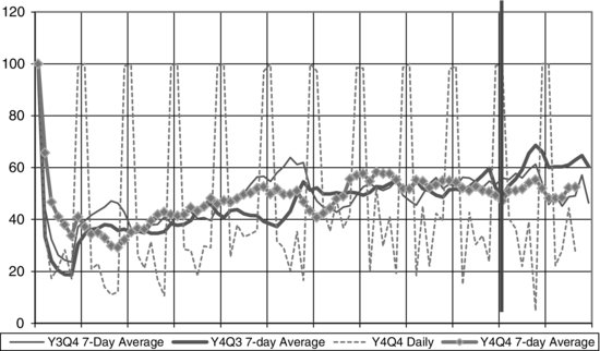
Figure 6.2 illustrates one of the dashboard displays used in the early quarter monitoring activities. The percentages of screener calls made during peak interviewing hours (weekday evenings and weekends) indicates the extent to which interviewers followed management staff instruction to seek informants when most likely to be at home. The figure shows daily as well as 7-day moving average percentages. Daily values were highly variable, and show system features that were not relevant to the management process, such as weekend reports (Saturday and Sunday) which are by default 100% of the calls anyway. The figure also allowed staff to compare performance across quarters, and intervene when a current quarter departs from past quarter performance.
FIGURE 6.1 The 2006–2010 NSFG dashboard.
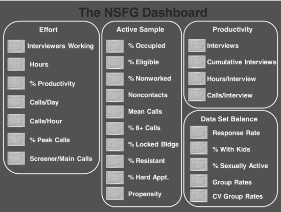
FIGURE 6.2 Early quarter graph example. Daily and 7-day moving percentage of screener calls made during peak hours.
Middle quarter (weeks 4--6) monitoring saw the focus change to monitoring the quality of the active sample, while continuing to examine effort. Here key indicators included the eligibility rate of sample addresses, the number of addresses found to be in locked buildings or gated communities, the level of resistance encountered at contacted addresses, calling levels, and sample line propensities.
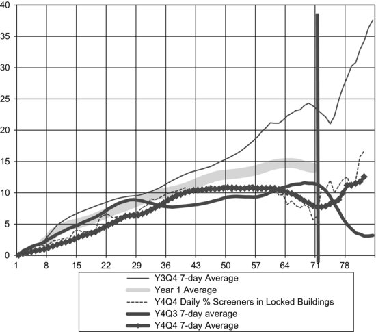
Figure 6.3 is an example of a middle quarter graph, the percent of active screener lines that were in locked buildings or gated communities to which interviewers could not gain access initially. Again, daily percentages are highly variable, so 7-day moving averages were presented as well. Across quarter comparisons could be readily made within the same year, and across years, and this particular figure includes a yearly average for additional contrast in monitoring. Year 4 results show lower levels of locked building lines than Year 3, because the sample blocks in Year 4 had fewer locked buildings and gated communities in them.
FIGURE 6.3 Middle quarter graph example. Daily percent active screener lines in locked buildings ((Ever locked until final disposition/All non-finalized cases)*100).
The late quarter (weeks 7--9) focus was on productivity and dataset balance. Key productivity indicators were interview counts, hours per interview, and calls per interview. Dataset balance indicators included subgroup response rates in an effort to reduce the risk of nonresponse bias.
Figure 6.4 illustrates one of the late quarter graphs utilized by management staff to monitor survey progress. The graph presents cumulative total counts, a more stable measure of survey performance since the count continues to accumulate and grow day by day. Results were deliberately separated by screener and main interviews; screener interviews are more numerous because they include households found not to contain eligible persons of age 15--44.
FIGURE 6.4 Late quarter graph example. Cumulative screeners and mains by day of data collection.
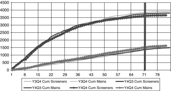
FIGURE 6.5 Selection of PSU’s for the 2006–2010 NSFG. Definitions: PSU – Primary sampling unit, NSR – Non-self-representing unit, SR – Self-representing unit, MSA – Metropolitan statistical area, Super 8---Eight largest MSAs.

With this paradata system in mind, the next section discusses the five key design changes in the 2006–2010 NSFG and how they were managed using paradata.
6.4 KEY DESIGN CHANGE 1: A NEW EMPLOYMENT MODEL
The continuous NSFG utilized an interviewer employment model in which interviewers were required to work 30 h per week. Instead of a group of over 250 interviewers in the field during data collection, the field staff for the 2006–2010 NSFG consisted of approximately 40 field researchers (interviewers) with direct supervision from two field operation coordinators. This small, elite team was experienced in all facets of the work required for NSFG, had proven success in field work, and had known leadership abilities. In addition, applicants who had a history of interest in the field of social sciences, either through education, past work experience, or through volunteer work were given special consideration.
Selecting the right staff was critical for this design, given that in most PSUs only one interviewer was employed in order to maintain effective central control. Therefore, the risk of attrition had to be minimized in order to avoid having unstaffed areas. The nearly full time employment required of each interviewer led to an interviewing staff that had less than 10% attrition in any given year, substantially less than the 40% attrition in the 2002–2003 NSFG.
Training occurred each year with a new group of recruited staff as the sample areas changed. The training was approximately 1 week and was designed to be hands-on with the systems needed to complete the work. Background lecture material was moved to DVD format and was completed at home before coming to in-person training. There was consistency of training across the years.
Supervising the two field operation coordinators was a field production manager who was the liaison with the management staff at the central office. The management staff was small, cross-functional, and in daily contact with field production staff. When new interviewers joined the project, they were asked to complete a “Field Researcher Questionnaire” in order to collect data on the characteristics of those collecting the data. The changes in focus of the 2006–2010 recruitment resulted in an trainee pool significantly more likely to have interviewing experience, have higher education, and more likely to say they liked approaching a household than the 2002–2003 trainees (see Table 6.1).
Table 6.1 Percent of 2002–2003 versus 2006–2010 NSFG Interviewer Trainees with Selected Characteristics
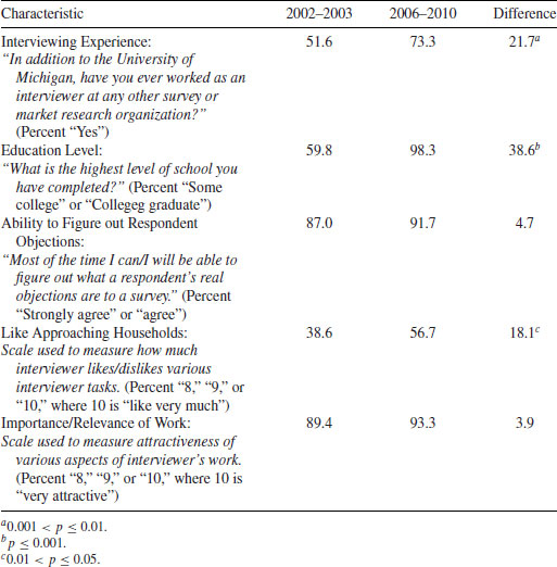
New paradata indicators were developed to monitor efficiency with the new employment model. For example, while it is always a requirement for interviewers to upload survey and operational data each day, a dashboard indicator was produced in order to monitor compliance on a daily basis and follow up with interviewers as necessary. This was important as the data in the dashboard indicators were only accurate if interviewers were sending updated information each day. In addition, indicators were developed to track whether interviewers were meeting the 30 h per week work commitment and reporting hours worked on a daily basis.
6.5 KEY DESIGN CHANGE 2: FIELD EFFICIENT SAMPLE DESIGN
For the sake of management efficiency, a portion of the NSFG sample was designed around interviewer productivity. In particular, with each annual and calendar quarter sample release, four key design parameter estimates were altered to change sample allocation across second stage sample units or segments (see Lepkowski et al., 2010). The sample sizes were varied by PSU and by quarter to respond to changing survey conditions. Thus, the sample size of addresses for an interviewer was not fixed to be the same across interviewers, but rather it was adjusted up or down based on recently available data. This is a form of responsive design – modifying key design features as the survey learns about the essential survey conditions encountered in a PSU.
The primary parameter in the allocation at the PSU and segment level was the interviewer workload. Interviewers were recruited and hired to work 30 h per week, 360 h in a 12-week quarter. Standard sampling theory suggests that clusters be allocated the same sample size, specifying sample size in terms of completed interviews. However, the practice has been to assign interviewers the same number of sample addresses, regardless of expected response and eligibility rates and their expected efficiency. Interviewers were expected to adjust their hours to accommodate the available work.
Interviewer work assignments in the 2006–2010 NSFG varied by the nature of the communities in which the work was assigned. Five factors varied from one work area, or PSU, to the next:
Consider two hypothetical PSUs in the 2006–2010 NSFG and how addresses would be allocated to each. Suppose each has a single interviewer who plans to work 360 h in the next quarter. From paradata, the expected hours per interview and the occupancy, eligibility, and response rate, for each PSU, were estimated. The estimation was based on rates observed in other similar PSUs in prior years, or if the PSU was in a later quarter during its year in the sample (see later), data from that PSU. In this case, suppose these two hypothetical PSUs are about to enter the first quarter of interviewing, and they are each similar to other PSUs where interviewing has been completed in a prior year. In one, interviewing was efficient, say 8 h per completed interview, and the other, 12 h per interview. Thus we would expect in the first PSU 360/8 = 45 completed interviews, and in the other 30 completed interviews.
In addition, for the first PSU suppose the expected occupancy rate was 80%, a household eligibility rate of 50%, and a response rate of 75%, while for the second the expected occupancy rate was 90%, a household eligibility rate of 60%, and a response rate of 90%. Then, for the first 45/(0.8 × 0.5 × 0.75) = 150 addresses were selected to provide an adequate workload for the interviewer, and in the second 30/(0.9 × 0.6 × 0.9) or about 62 addresses. Different numbers of completed interviews were expected in each PSU, but the effort required by the interviewers was expected to be about the same. This allocation process led to variation in probabilities of selection of housing units across segments within and among PSUs, and variation in sample size across PSUs in the same strata. The variation in sampling rates was compensated for in the weighting process, although the added variability in sample weights from varying line probabilities at the segment level had the potential to increase the variability of survey estimates. The variation in number of completed interviews was accounted for through the variance estimation procedure.
6.6 KEY DESIGN CHANGE 3: REPLICATE SAMPLE DESIGN
The continuous design spread the work previously done in 11 months across 4 years. A sample design was needed that provided a similar number of PSUs as were selected in the previous 2002–2003 NSFG, but the 2006–2010 employment model required that the workloads in a year in a PSU be about the same as experienced in 2002–2003. Maintaining the same number of PSUs and sample sizes per PSU meant that the 2006–2010 NSFG needed a way to spread the PSUs over time, over the 4 years. In effect, the continuous design coupled with the employment model required that the PSU sample be selected not only across space (the geography of the United States) but also across time.
A sample of 110 PSUs was selected for the 2006–2010 NSFG national sample, and then these PSUs were “subsampled” or divided into four national samples. This subsampling yielded an equivalent to what is referred to in the survey sampling literature as replicated sampling; repeating the sample selection multiple times. Each of the national samples was subsequently assigned to one of the 4 years of interviewing.
The 110 PSUs were, for purposes of identification, grouped into four types: (1) the eight largest metropolitan areas among the 28 self-representing (SR) areas, (2) the remaining 20 largest self-representing metropolitan areas, (3) 52 non-self representing (NSR) but also metropolitan areas, and (4) 30 NSR but non-metropolitan areas. This grouping was then used in the division of the sample of 110 PSUs into four fully representative national samples for the 2006–2010 NSFG (see Figure 6.5). Each annual national quarter sample consisted of:
- All eight of the largest SR metropolitan areas, referred to as the “super eight PSUs,” that were, because of size, always in the sample.
- Five of the remaining 20 SR metropolitan areas selected carefully to represent the full set of 20 in each year.
- Twenty (or 22, in the first year) NSR metropolitan and non-metropolitan areas selected to represent the full set of 82 NSR PSUs in each year.
The smaller national samples provided an opportunity to more effectively monitor field data collection and cost, and operate with a smaller central office staff. These four national samples allowed the production team to make changes, as required, to data collection, survey questions, and other design features once each year. In addition, the four replicate samples could be combined across years to yield larger sample sizes across longer multi-year time periods.
6.7 KEY DESIGN CHANGE 4: RESPONSIVE DESIGN SAMPLING OF NONRESPONDENTS IN A SECOND PHASE
Data collection was completed in a series of four quarters each year, each quarter lasting 12 weeks. The first 10 weeks of the quarter was “phase 1” of the study and the last 2 weeks of the quarter was “phase 2”. In phase 1, normal protocols applied. Selected housing units were screened for eligibility and, when eligible, interviewed. In week 10, the outstanding sample was reviewed and a sub-selection of the remaining active lines were designated for phase 2. Typically, 30% of the remaining lines were selected for continuation in the second phase.
This was part of a two-phase sample design for nonresponse. Two-phase samples for nonresponse are increasingly attractive to survey researchers because they offer a way to control the costs at the end of a data collection period while addressing concerns about nonresponse rates and errors. At the end of the data collection period, large costs are incurred for travel to sample segments to visit only one or two sample units, usually those extremely difficult to contact in prior visits or with concerns about the survey request. By restricting these expensive visits to a sample of the nonrespondents at the end of the study, a more cost-effective method limits costs while addressing the need to increase response rates.
The second phase sample selection relied in part on paradata-derived measures of response propensity. At the end of phase 1, a random selection of two-thirds of the second stage units or segments in each PSU was selected for phase 2. Then the daily propensity model was estimated for each of the remaining outstanding cases, and the predicted probability of response the next day calculated for each active case. These active cases were stratified by likelihood of response (high and low) and by type of case (screener or main). Those with a higher likelihood to respond were oversampled.
In phase 2, only the sub-selected lines were released to interviewers in the sample management system. All other cases were dropped out of the sample, although a compensating weight was incorporated into the final weight to account for this subsampling. In addition, a change in recruitment protocol was implemented. Adults in the second phase sample were given an increased token of appreciation (from $40 to $80), and interviewers were allowed to use proxy reporters for the completion of screeners. There was also a change in interviewer behavior as well, with all of the interviewer effort applied to very few cases in order to maximize response rates with the remaining cases. Figure 6.6 provides an illustration of the trends in the number of remaining cases throughout the first phase and into the second phase subsample. It also shows the trend in response rates, and, after the second phase sample, the gain in a weighted response rate computed as a result of the two-phase sampling strategy.
FIGURE 6.6 Illustration of second phase sample and response rate.
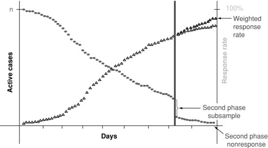
There are advantages and disadvantages to the use of a two-phase sample in data collection. The advantages include control over work effort for high effort cases, control over costs, and change of recruitment protocol. The disadvantages include the need for additional weights to compensate for the second phase selection and potentially higher sampling variance in resulting estimates.
6.8 KEY DESIGN CHANGE 5: ACTIVE RESPONSIVE DESIGN INTERVENTIONS
Groves and Heeringa (2006, p. 440) define responsive design as follows: “The ability to monitor continually the streams of process data and survey data creates the opportunity to alter the design during the course of data collection to improve survey cost efficiency and to achieve more precise, less biased estimates.” Such surveys are labeled as responsive designs. These designs have the following characteristics:
Responsive design requires active management of the field effort through the use of paradata and paradata monitoring. With responsive design, interviewer effort is used with maximum effectiveness and study procedures can be changed in response to changing field conditions. The effects of these changes (“interventions”) can be documented by paradata.
As described previously, the NSFG oversampled certain populations, such as Hispanics, Blacks, and teens, in order to have sufficient completed interviews for estimation. One type of responsive design intervention on NSFG involved targeting a specific subgroup of active sample cases found to have poor or lagging values on key process indicators. For example, Figure 6.7 shows that between days 1 and 43 of Quarter 14, older (ages 20--44) male Hispanics were lagging in terms of response rates. In response to this observed trend (monitored daily from the NSFG dashboard), NSFG mangers implemented an intervention designed to have interviewers target sample in this specific subgroup. This intervention began on day 44 of the quarter, with targeted older male Hispanic sample flagged in the sample management system. Figure 6.7 shows the relatively sharp increase in response rates within this subgroup over the next week. This intervention had the beneficial effect of decreasing the variation in the response rates among subgroups. The variation in response rates across key subgroups was a very important process indicator monitored by NSFG managers to assess balance in the dataset. After this intervention was completed, the variation in the response rates remained stable for the remainder of the quarter.
FIGURE 6.7 Daily response rates for six key subgroups for one quarter, 2006–2010 NSFG.
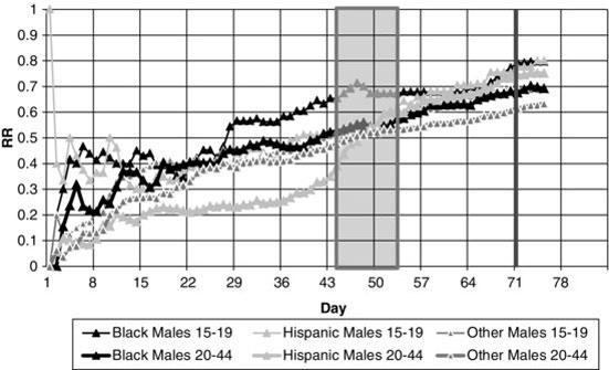
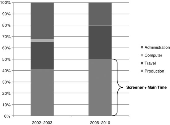
FIGURE 6.8 2002–2003 NSFG versus continuous 2006–2010 NSFG distribution of interviewer time.
6.9 CONCLUDING REMARKS
The change from a one-time, large-scale data collection effort to a smaller, continuous design required changes in the employment model for interviewers, sample design, paradata monitoring techniques, and the use of responsive design. These changes resulted in the successful implementation of the 2006–2010 NSFG continuous data collection, with an increase in field efficiency contributing to higher than anticipated interview yield. An example of the increase in field efficiency between the 2002–2003 and 2006–2010 NSFG surveys is the distribution of interviewer hours across various tasks (see Figure 6.8). In 2002–2003, about 40% of interviewer hours were spent on screening and interviewing. The remainder of the hours were spent on non-production activities such as administration, travel, and computer problems. In 2006–2010, about 55% of interviewer hours were spent in screening and interviewing.
Another example of the gains in efficiency is demonstrated by the hours per interview. The hours per interview is calculated by the sum of the interviewer hours divided by the total number of interviews collected. The hours encompass all of the tasks necessary to complete the work---administrative, travel, screening households, and conducting interviews. For 2002–2003, each completed main interview required an average of 11.3 h of work. In 2006--2010 with the continuous design, the achieved hours per interview averaged 9.0 h. It is worth noting that other operational refinements to the data collection protocols were put into place for continuous interviewing which also contributed to the improvement in efficiency and cost savings. For example, tablet computers were used for electronic listing of sample segments and for obtaining electronic signatures on consent forms. Using tablet computers for these tasks eliminated the need for paper processing of sample lists and consent forms at headquarters.
The increased efficiency realized through the continuous interviewing design resulted in a 79% increase in interview yield between the two surveys. In 2002–2003, there were 12,571 main interviews collected in an 11-month data collection period from March, 2002 to February, 2003 with a response rate of 78%. In 2006–2010, there were approximately 22,500 main interviews collected in a data collection effort spanning 4 years, from July, 2006 to June, 2010, with a response rate of 76%. The cost expended in these two efforts was approximately the same. Thus, a redesign that relied, in part, on paradata led to a more efficient survey data collection on the same survey. Paradata have also been instrumental throughout the 2006–2010 NSFG in improving the efficiency of the sample design.
There are two critical questions that remain. While we cannot prove conclusively that paradata led to the kinds of gains in efficiency indicated here, we believe that the evidence across the five key design changes discussed points clearly to the value of paradata in design and responsive design of sample surveys. Second, we have yet to show whether these kinds of design changes improved data quality. We have indirect evidence (not shown here) that several 2006–2010 NSFG design features have reduced nonresponse bias. Nonetheless, further work remains to show that these efforts do lead to reduced error in estimates.
REFERENCES
Botman, S., Moore, T., Moriarity, C., and Parsons, V. (2000). Design and Estimation for the National Health Interview Survey, 1995–2004. National Center for Health Statistics. Vital Health Statistics, Series 2, 130.
Groves, R., Fowler Jr., F., Couper, M., Lepkowski, J., Singer, E., and Tourangeau, R. (2004). Survey Methodology. Wiley and Sons, Inc., Hoboken, NJ.
Groves, R., Mosher, W., Lepkowski, J., and Kirgis, N. (2009). Planning and Development of the Continuous National Survey of Family Growth. National Center for Health Statistics, Vital Health Statistics, Series 1, 1(48).
Groves, R.M., Benson, G., and Mosher, W.D. (2005). Plan and Operation of Cycle 6 of the National Survey of Family Growth. National Center for Health Statistics, Vital Health Statistics, Series 1, 42.
Groves, R.M. and Couper, M. (1998). Nonresponse in Household Interview Surveys. Wiley and Sons, Inc., New York.
Groves, R.M. and Heeringa, S.G. (2006). Responsive Design for Household Surveys: Tools for Actively Controlling Survey Nonresponse and Costs. Journal of the Royal Statistical Society, Series A, 169(3):439–457.
Hansen, M.H. and Hurwitz, W.N. (1946). The Problem of Nonresponse in Sample Surveys. Journal of the ASA, 41(236):517–529.
Kish, L. (1995). Survey Sampling. Wiley and Sons, Inc., New York.
Lepkowski, J., Mosher, W., Davis, K., Groves, R., van Hoewyk, J., and Willem, J. (2006). National Survey of Family Growth, Cycle 6: Sample Design, Weighting, Imputation, and Variance Estimation. National Center for Health Statistics. Vital Health Statistics, Series 2, 142:1–82.
Lepkowski, J.M., Mosher, W.D., Davis, K.E., Groves, R.M., and Van Hoewyk, J. (2010). The 2006–2010 National Survey of Family Growth: Sample Design and Analysis of a Continuous Survey. National Center for Health Statistics. Vital Health Statistics, Series 2, (150).
Mosher, W.D., and Bachrach, C.A. (1996). Understanding United States Fertility: Continuity and Change in the National Survey of Family Growth, 1988–1995. Family Planning Perspectives, 28(1).
Singer, E. (2006). Nonresponse Bias in Household Surveys. Public Opinion Quarterly, 70(5):637–645.
U.S. Census Bureau (2009). Design and Methodology, American Community Survey. Technical report, U.S. Government Printing Office, Washington, DC.