CHAPTER 10
Computer System Storage Fundamentals
Before you can dive head first into exciting investigations involving computer intrusions from foreign countries, international money-laundering schemes, foreign state-sponsored agents, or who posted your purity test score to Usenet, you need to have a solid understanding of basic computer hardware, software, and operating systems. In this chapter, we focus on system storage—hard drives and the file systems on those drives. If you can answer the following three questions, skip ahead to Chapter 11.
This chapter begins with an overview of the various hard drive interface standards and how they affect your forensic duplications (including how to avoid the destruction of expensive SCSI hardware). Then it covers how to prepare hard drive media for use during your investigation. The final section introduces the principles and organization of data storage.
There are few situations more frustrating than preparing to run a few quick searches on your forensic duplicate, but running into technical difficulties at every step of the way. Understanding the hardware and the set of standards to which the system was built will significantly cut down the number of branches in your troubleshooting matrix.
In this section, we are going to quickly cover the basics of hard drive interface formats. The term interface is a bit of a misnomer here. We are compressing the concepts of interfaces, standards, and protocols into one section in an effort to simplify the discussion. (For more details on hard drives and other computer hardware, refer to a book on that subject, such as Scott Meuller’s Upgrading and Repairing PCs, published by Que.)
IDE/ATA (Integrated Drive Electronics/AT Attachment) and SCSI (Small Computer System Interface) are the two interface standards that most computer forensic analysts will encounter. IDE drives are cheap, simple to acquire, and have a respectable transfer rate. SCSI drives move data faster than IDE/ATA drives, but at a much higher cost.
The ATA interface started out as a fairly simple standard. ATA-1 was designed with a single data channel that could support two hard drives, one jumpered as master and the other as slave. This standard supported programmed I/O (PIO) modes 0 through 2, yielding a maximum transfer rate of 8.3MB/second. The next big improvement came with the adoption of direct memory access (DMA) usage. Using the DMA method allowed the computer to transfer data without spending precious CPU cycles. A short amount of time went by, and the speed increases (up to 16MB/second) became insufficient. The standard evolved into a higher-speed version known as Ultra-DMA.
The current iteration is Ultra-DMA mode 5, which boasts a maximum transfer rate of 100MB/second. The previous three modes transferred data at MB/second rates of 66,44, and 33, giving us the explanation behind the labels printed on hard drive packages: ATA/33, ATA/44, ATA/66, or ATA/100. (ATA/44 caught on for only a short time; we have yet to encounter these drives, but they allegedly exist.) An important fact for forensic analysts in the field is that the IDE/ATA modes are backward-compatible.
Drive Size Boundaries
Along with the rate of data transfer, the growing size of drive media is also a concern for the T13 committee (the group that releases ATA standards). At the time of this writing, Western Digital sells 200GB hard drives. Unfortunately, the ATA controllers on the market are not able to handle anything over 137GB. Drive manufacturers are packaging ATA interface cards that are built upon draft specifications (UDMA Mode 6). When the T13 committee ratifies the updated standard, these ATA interfaces will replace the current versions built onto motherboards and PCI cards. This works fine in an office or laboratory environment, but you may be out of luck when acquiring images on systems that are not under your control. The current ATA interface standard uses 28-bit addressing, which tops out at approximately 137.4GB. Furthermore, operating system utilities such as Microsoft’s Scandisk and Disk Defragmenter do not currently operate properly on drives over 137GB, even if the ATA controller card is updated.
Previous drive media size boundaries have been at 32GB, 8.4GB, and 2.1GB. Time will sort these problems out, but it serves as a warning to labs that attempt to purchase cutting-edge hardware.
Drive Cabling
How do the ATA standards apply to forensic duplication? One of the goals of efficient duplication is to get the maximum amount of data safely transferred in the least amount of time. Proper cabling plays an important role in achieving these goals. The following sections discuss a few key points regarding the cabling for your evidence media.
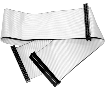
Cable Requirements Up until the ATA/33 standard, a 40-conductor/40-pin cable was sufficient. Figure 10-1 shows a 40-conductor/40-pin ribbon cable.
Anything faster than ATA/33 requires an 80-conductor/40-pin cable, such as the one shown in Figure 10-2. This newer cable has several attributes that correct problems with the old version. First, the presence of 40 more conductors minimizes the amount of interference and crosstalk between the 40 active wires. The extra 40 conductors are tied to the ground pin on the connector to act as a drain for any excessive current. Second, the connectors are color-coded as blue, gray, and black. Each one has a specific role:

If you ignore these color codes, you may have problems with the BIOS not recognizing a hard drive, or worse, data corruption. Placing a single drive on the middle connector leaves a pigtail of unterminated wire that will result in reflected signals and degradation in signal quality.
Mixed Hard Drive Types You can place drives with different ratings on the same cable. If you are using an ATA/100 host controller and have ATA/33 and ATA/100 hard drives connected via an 80-conductor cable, each drive will perform at its rated speed. And if you have an ATA/33 host controller with ATA/33 and ATA/100 hard drives, the fastest transfer speed you could attain would be approximately 33MB/second.
Mixed Cable Types Mixing cable types is a proven way to cause problems. If you must daisy-chain IDE cables (not exceeding the 18-inch limit), ensure that both cables are of the identical type. The ATA host controller will detect the type of cable connected to each bus by checking the PDIAG-CBLID signal on pin 34. (The PDIAG-CBLID pin is the Passed Diagnostics-Cable Assembly Type Identifier, just so you know if it ever comes up in a future Jeopardy show.) If pin 34 is tied to ground, the controller knows that an 80-conductor cable is attached. Incidentally, this is also why it is important to make sure that the blue connector is mated with the host controller, because this is where the pin is grounded.
You may be wondering when the problem of mixed cable types may arise. Until recently, companies that assemble computer systems for forensic use have had a hard time finding a source for an 80-conductor version of the short “extension cable” that allowed them to place a male IDE connector on the back of the computer system. We observed several situations where an 80-conductor cable was mated to the backplane, causing the host controller to go into ATA/100 mode. Because of the lack of shielding on the 40-conductor cable inside the computer, the BIOS had intermittent problems identifying external drives. Figure 10-3 illustrates this condition.

Cable Select Mode If you are a fan of the cable select mode capability, you finally have something to cheer about. The entire IDE/ATA system is now designed for cable select mode to operate as initially planned (assuming the hard drives themselves cooperate). This mode allows the user to place the hard drives on the ATA cable without setting jumpers. One would place the master at the end of the cable, and the slave at the midpoint. We are fans of making things behave in a predictable manner, so we usually lock the drives down to master and slave by setting the jumpers to the manufacturer’s specifications. These specifications may be found printed on the label or in the documentation included with the hard drive.
ATA Bridges
There are a multitude of reasons for using ATA host bridges, such as IDE-to-SCSI, IDE-to-IEEE 1394 (FireWire), and IDE-to-USB 1.1 or 2.0 bridges. For forensic examiners, the two primary benefits of using an ATA host bridge are the availability of hardware-based write protection and the capability to hot-swap hard drive media.
In the past, we protected hard drives from alteration by using software-based interrupt 13 write-protection programs. Although this approach worked quite well during Safeback and Snapback duplication sessions, it was widely known that there were other methods of writing to a disk that did not use DOS-based interrupts. Several companies began offering products that would intercept data transferred to the drive during write operations. The concept of ATA bridges made this solution easier to implement.
If you are able to add ATA host bridges to your toolkit, you should purchase models that convert to IEEE 1394 (FireWire) or USB 2.0 and are compatible with your processing environment (Windows or Unix). Some manufacturers have engineered interfaces that have a hardware-based write protection feature. We strongly recommend adding this extra layer of protection to your evidence processing workflow.
GO GET IT ON THE WEB
WiebeTech ATA-to-FireWire bridges: http://wiebetech.com Forensic-Computers ATA-to-FireWire bridges: http://www.forensic-computers.com
SCSI has long been the interface of choice for server-class computer systems, RAID (Redundant Array of Independent Disks) devices, and Apple computers. Most of the time, you will deal with ATA/IDE devices, both in the field and in your lab. However, it is important to understand SCSI and how it differs from the ATA standard, on paper and in practice.
The difference in data throughput between ATA and SCSI is very small. Typically, drive manufacturers will use the same head-and-platter assembly on both product lines and simply attach the appropriate controller card. While the external transfer rate for the SCSI version may approach 320MB/second (three times more than the current ATA technology), the internal transfer rates (from the platters to the interface) are the same.
You will begin to notice the advantages of SCSI when multiple devices are present on the SCSI bus. ATA devices will take over the entire bus for the duration of a read or write operation. Only one ATA device can be active at a time on each ATA bus. SCSI supports parallel, queued commands where multiple devices can be used at once, if the operating system supports it. This is one reason that SCSI RAIDs will outperform ATA RAIDs when they are under a heavy I/O load.
Speaking of multiple devices, SCSI signal chains may hold up to 7 or 14 devices. One device ID is reserved for the SCSI controller card (typically SCSI ID 7). SCSI devices may also be further divided into logical functional subelements. The subelements are addressed with Logical Unit Numbers (LUNs). Most tape backup devices with multiple-tape cassettes (including expensive robotic arm models) will use separate LUNs to control the tape drive and storage management device.
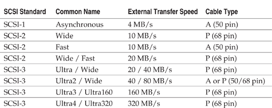
The ANSI standards board responsible for SCSI standards has released three implementation specifications: SCSI-1, SCSI-2, and SCSI-3. Table 10-1 lists the major SCSI standards and their common names. All of the standards are backward-compatible, so you can purchase the latest full-featured SCSI adapter and have the ability to handle older devices.
TIP
We suggest the Adaptec Host Adapter 2940 Ultra (aic7xxx) card. We have used it for years with no problems, and drivers are available for nearly every operating system.
SCSI Signaling Types
There are a few ways to unintentionally completely destroy computer hardware. For SCSI devices, mixing devices designed for different bus types is a sure way to turn them into useless doorstops. If you thought it was difficult to procure the funds for a $1,500 8mm DAT tape drive, try to get it replaced after filling your lab with that unmistakable smell of burnt silicon.
The four SCSI signaling types that you need to recognize are listed here, along with the symbols found on the device.

Single-ended Signaling The original SCSI specification called for single-ended (SE) signaling. This method used a pair of wires for every signal path: one wire for signaling and the other wire tied to the ground connection. This implementation was prone to interference and data corruption problems. Due to the level of interference, the implementation calls for short cable lengths, typically less than 5 feet (1.5 meters).
High-Voltage Differential Signaling The alternative to SE signaling was high-voltage differential (HVD) signaling. To eliminate the interference problems, the SCSI specification boosted the voltages on the wires significantly and began to carry the inverse of the signal on the second wire in each pair. These HVD interfaces were more expensive, and they were used primarily on microcomputers. It is unlikely that you will run across these devices.
Low-Voltage Differential Signaling Low-voltage differential (LVD) signaling was created to strike an economical balance between SE and HVD signaling. The principles are the same as the HVD interface, but with a voltage low enough to avoid damaging devices that do not completely adhere to the LVD standard.
Low-Voltage Differential/Multimode Signaling LVD/SE, or Multimode, devices are compatible with SE or LVD signaling. Most devices on the market today will be LVD/SE.
CAUTION
Do not connect LVD or SE devices into a host adapter that is HVD. Doing so will render your hardware useless.
SCSI Cables and Connectors
SCSI cables are similar to motorcycle helmets; you could protect yourself with a $150 helmet, but you get what you pay for. Simply put, buy the best you can find. Do not settle for the stuff you can get out of the cable bin from the local computer swap meet.
Table 10-1, shown earlier, lists the cables required for each standard. The cables are divided into two types:
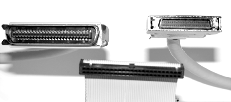

Be careful when you mix devices with different bit widths. When you mix the cable types by using 50-pin to 68-pin adapter plugs, the throughput of the entire chain will drop to the lower rate.
SCSI Termination
Any time that signaling cables use a relatively high voltage to transfer information, they are susceptible to signal reflection from the end of the cable. Unlike with ATA/IDE buses, you need to take an active role in ensuring the bus is terminated at both ends. Most SCSI adapters and internal hard drives have built-in termination that becomes active if the device detects that it is on the end of the SCSI bus. Table 10-2 lists the types of termination plugs required for each SCSI signaling type (SE, LVD, and HVD). Similar to SCSI cables, money should not be an issue when selecting terminators! The better the terminators, the fewer problems you will have.
| Signaling Type | Terminator Type |
| Single-Ended |
Passive Termination
Active Termination
Forced-Perfect Termination
|
| Low Voltage Differential or Multimode | LVD Termination |
| High Voltage Differential | HVD Termination |
NOTE
You have a choice only when using an SE bus. Although passive termination is listed, avoid it if you can. Use forced-perfect terminators (FPT) whenever possible, because they will ensure a low level of signal reflection, regardless of cable length.
As we’ve stated repeatedly in previous chapters, preparation is key to incident response. The hard drive of a computer that you will use for forensic analysis is no exception—you can prepare a hard drive so that it is ready for storage when you need it.
Our bench stock of storage drives currently consists of approximately ten 120GB hard drives that are wiped, partitioned, and formatted. This saves us a significant amount of time during a crisis. Our experience has shown that the most flexible configuration for a new drive includes a series of 20GB FAT32 partitions. This will allow the responder to use nearly any tool for duplication and analysis, without worrying about whether an operating system will be unable to access the storage medium.
First, we will cover how to wipe all data off of a drive, and then we will talk about partitioning and formatting.
At one time, wiping data off a hard drive was one of the most important steps in drive preparation. Back in the days when Safeback and Snapback were the only options, you needed to restore the qualified forensic duplicates before you could conduct your analysis. If you had used a hard drive for a previous case and not cleaned it, you would have had the potential for cross-contamination of the evidence. It would have been difficult to explain why four cases in a row contained the same suicide note.
Wiping storage media is less important today, given the more advanced methods of analysis available. With true forensic duplicates and forensic-processing suites, we are no longer required to restore the images, except in special circumstances. When analysis is performed through virtual disk mounting, the nature of the duplicate image file will keep old data from falling within the scope of your investigation. The Linux Loopback device, OnTrack’s Forensic Toolkit, ASRData’s S.M.A.R.T. suite, and Guidance Software’s En-Case use virtual disks to expose the evidence files to the examiner. In Chapter 11, we will cover the basic analysis techniques in a few of these environments.
The most preferable method to use to clean off storage media is the Unix dd command. The dd command will copy blocks of data from its “in file” to its “out file.” In this case, we use the /dev/zero device as the source, because this will give us a continuous source of NULL values (hexadecimal character 0x00). The following command line will wipe out any data on the second hard drive (/dev/hdb) in a Linux environment.
A better choice under Linux is the Department of Defense Computer Forensics Laboratory (DCFL) version of dd. This will show you how much data is transferred as it proceeds (essential in timing trips to Starbucks). The following is the equivalent command line for
dcfldd:
Our experience has shown that the most flexible partitioning scheme consists of a series of 20GB FAT32 partitions. This will allow the investigator to collect forensic duplicates under DOS (using EnCase or Safeback, for example) or Unix (using dd or
dcfldd). There are a few ways to quickly partition and format a drive. We will quickly cover the process under Windows XP and Linux.For the most reliable results when formatting a partition, use the operating system that is native to the format that you intend to use. We will typically use a Windows operating system to create FAT32 partitions to make sure that the partitions lie on cylinder boundaries. This will ensure the greatest degree of portability. Some operating system tools (such as Linux’s
fdisk) may fail to behave correctly when the boundaries do not match.Partitioning and Formatting Drives with Windows XP
Once the hard drive (we’ll call it the storage drive) is connected to the computer system and has been recognized by the BIOS, you are ready to proceed into Windows XP. Allow the system to boot, and enter the Disk Management applet, under the Computer Management portion of the Control Panel. Another route to the applet is to right-click My Computer, select Manage, and then choose Disk Management.
Ensure that the storage drive has been recognized. The Disk Management console should look similar to Figure 10-6. Right-click the drive and select Create Partition. Step through the Create Partition Wizard and create a single primary partition.

When you get to the point where you choose to format the drive, select FAT32 and make sure that the Quick Format option is checked. As the first partition begins to format, you can create the extended partition and the logical drives within it. Avoid creating multiple primary partitions. There are only four available in the Master Boot Record, and once you fill them all in, you’ll have to repartition to gain access to more. Figure 10-7 shows the formatting options available under Windows XP.

Partitioning and Formatting with Linux
You can verify that the hard drive (target drive) has been recognized by the BIOS and the operating system by running the
dmesg command. In the following example, we display all ATA hard drives by running the output of the dmesg command through grep, searching for hd. Notice that the manufacturer named in the example is CntxCorpHD. This is typically the value from the drive itself—Maxtor, Seagate, and so on.
This example shows that we have two ATA disk drives, named hda and hdb, connected to the computer. It also shows that Linux recognizes the partition tables on the drive. Two lines in the example display the partition labels:
Linux recognized that three partitions exist on the first drive and zero partitions are on the second (we just wiped it clean of any data).
NOTE
You may run into situations where Linux fails to recognize partitions on media that you know have valid tables. To minimize the likelihood of this occurring, recompile the Linux kernel and enable all partition types in the kernel options scripts. Further investigation may be required through the use of hex editors if valid tables are not recognized.
In this example, /dev/hdb is our storage drive. Run the
fdisk command to partition the drive. Once the utility has started, press P to print the contents of the current partition table. In the example below, the table is empty, since we wiped the contents of the drive.
Create a new partition by using the new partition command (press N). Select the option to create a primary partition, and enter the starting and ending cylinders. If you are creating multiple partitions, keep FAT32 partitions below 20GB and create only one primary partition with multiple logical drives in the extended partition.
The
fdisk command will set the system type on any new partitions to type 81, Linux. You will need to use the option to change a partition’s system ID (press T) to change it to an MS DOS type. You will typically use types B and C for large FAT32 partitions. The following example shows what the partition table will look like after creating a single 15GB
Press W to commit the changes. Then exit
fdisk when you are finished. The last step is to format the FAT32 partition. Use the mkfs command to create new file systems. The command below will format the new partition in our example, /dev/hdb1.When it is complete, the new file system is ready to be used. The next section offers an introduction to how file systems store data.
Knowing where evidence resides on data storage media is essential to successful forensic analysis. You can view the file system as a layered model, similar to the OSI networking model. As shown in Figure 10-8, we identify six layers of the file system:

You will find information of evidentiary value at each of these layers. Keeping these layers in mind during your analysis may help you to determine the correct type of tool to use to extract the information that you need, as well as to identify the information that a particular tool will not be able to recover.
The lowest level of file storage is the physical layer, which is always present, regardless of the operating systems or file systems that are on the hard drive. The machine will read and write to the hard drive in blocks (sectors). Most operating systems that you will run across will read and write in 512-byte chunks.
Absolute sectors are numbered sequentially, starting at zero and continuing until the end of the drive. If you end up working on a case where the parties involved have a high degree of sophistication, you can force the duplication software to ignore what it detects as the last absolute sector and continue until it receives error codes from the hard drive. Quite often, a track or two will be reserved for use by the hard drive itself, and it is possible to store a small amount of data there. Intel hardware exposes an additional interface that uses three values (cylinder, head, and sector) to locate a specific portion of the disk. If you need to perform data recovery, it will be advantageous to become familiar with how the C/H/S system works.
Just above the physical layer lies the partitioning scheme set up by the operating system. This scheme allows the user to segregate information in the interest of security (operating system on its own partition), file system optimization (smaller partitions may speed file system access), or just plain organization (keeping work and music archives separate, for example). On Unix installations created on servers (web servers or email servers), different types of data are kept in separate partitions. This allows the operating system to run reliably, regardless of how quickly the mail spool or log files are filled by traffic.
On creation, the partition will be assigned a partition identifier. This single-byte code will tell an operating system what kind of file system to expect, in case it wants to mount the partition. An interesting tactic of some boot managers is marking unwanted partitions with an invalid code. If Windows observes an unknown partition-type ID, it will completely ignore the partition, even if it is formatted correctly and has valid data.
GO GET IT ON THE WEB
List of partition identifiers: http://www.win.tue.nl/~aeb/partitions/partition_types-1.html
Most Unix variants will use the term slice instead of partition. The concepts are similar, but they are different in implementation. In order to remain compatible with the Intel partitioning specification, BSD partition tables and slices are encapsulated within a standard partitioning scheme. For example, this means that the entire file system for a new installation of FreeBSD on an Intel-based computer will actually reside within the first partition on the hard drive. At the beginning of that primary partition, BSD will place a table that subdivides that area into BSD-style partitions. Figure 10-9 is an example of this type of partition-table encapsulation. If you are performing forensic analysis under Linux, be sure to recompile your kernel, adding in the BSD partitions option.

GO GET IT ON THE WEB
Compiling a New Linux Kernel: http://www.tldp.org/index.html
The next level of file system storage refers to the blocking, or the allocation method, used by the operating system. The size of each allocation unit depends on three variables: the type of file system, the size of the partition, and the knowledge of the system administrator.
Each file system defines its own scheme for laying out data on the storage medium. Most use a block size that is optimized for the size of the partition. Table 10-3 shows the most common sizes for allocation units. The FAT standards migrated from inefficient static values (4KB per block) to a sliding scale. Developers have attempted to strike a balance between a large number of small blocks, a scheme that uses space more efficiently, and a smaller number of large blocks, where the file system may be faster during search and transfer operations.

The system administrator has the option to override the default block sizes in certain situations. For example, if a Unix server is expected to use drive space in large blocks (such as would be the case on database servers) and few small-sized files, the administrator may see an increase in speed if she creates the file system with an 8KB block size. This information is stored in special tables throughout the file system, and it can be retrieved if needed for data-recovery operations.
The storage space management layer lies above the allocation units layer in our classification system. This layer manages the thousands of allocation units present on a file system, where the allocation unit is the smallest addressable chunk of data that the operating system can handle. Think of this as a map that shows you which parking spots are occupied in a huge garage. On FAT file systems, there are two of these maps, and they are kept in sync by the operating system. Other file systems will split a partition into sections and will maintain a single mapping table for each section.
FAT file systems use a file allocation table (the FAT) to keep track of the status of every allocation unit on the file system. By observing the value contained in the table for a particular unit (in the case of DOS, these are also called clusters), you can tell if the cluster is in use, if there are additional units in the chain, if it is the end of the chain, or if it contains bad blocks. To illustrate this concept, Figure 10-10 represents a small portion of the FAT. This file system was created with an allocation unit size of 2048 bytes. We have performed the following operations on the file system:

Notice how the storage space management table is simply a “chain” for the operating system to follow when reconstructing a file. In a FAT-based file system, each block may have one of three values:
In the example shown in Figure 10-10, we created a fragmented file (TEST1.txt) by closing the file handle associated with TEST1.txt (we stopped writing after 4659 bytes), started a new file (TEST2.txt), and then appended more data to the first file (TEST1.txt). Modern file systems work on a similar concept where data blocks are allocated as they are requested by the operating system, but have methods to reduce the amount of fragmentation that occurs when saving modified files.
The top two layers of the file system storage model consist of directories and files. These are the levels that are familiar to most users. These layers are defined by the operating system in use on that partition. Several types of files are significant to a forensic investigation:
Generally, you can reduce the number of files that require examination by comparing hash values to known-good file lists. These known-good lists are compiled from original operating system installations and application files. Another method used to minimize spurious data is elimination based on file timestamps. Once the investigation has come to a point where you are isolating events occurring within a certain time frame, you can use complete file listings to estimate events that occurred on the system. The techniques for analyzing data at the information, classification, and application level storage layers are detailed in Chapters 11, 12, and 13.
The information about hard disk and file system storage presented in this chapter simply allows the investigator to get to the point of analysis quickly. Invariably, hardware problems will arise, regardless of how many thousands of dollars you spend on a forensic workstation. Evidence media will refuse to be identified by the BIOS; SCSI devices will fail to be completely functional; and operating systems will fail to recognize partitions that you know are there. Knowing how hard drives and file system storage work is often more important than experience with commercial forensic software. The principle is simple: The more familiar you are with how the system works and what can go wrong, the more prepared you will be to deal with unexpected issues and failures.
In the next chapter, we will review the tools you need to assemble the information stored on a hard drive. Specifically, you will learn to perform the steps taken before interpretation of the data.
1. A partition on an ATA hard drive is not recognized on your forensics workstation, which is running Linux. What troubleshooting steps should be taken? What order should they go in? What would you do under Windows 2000/XP?
2. You have booted up your forensic workstation, and a SCSI hard drive connected to the external chain is not detected. How would you resolve this?
3. From the description of the file system layers, what would be the process for identifying unallocated space on a drive? How would you identify slack space (RAM and file slack)?
4. Name five methods for hiding data on a hard drive, using the layers below the information classification layer only. How would you, as an examiner, detect these conditions?
..................Content has been hidden....................
You can't read the all page of ebook, please click here login for view all page.