

Sum of Extremes Test
This appendix provides a more detailed and clearer explanation of the sum of extremes test than is contained in Chapter 7. The goal of this appendix is to answer all your questions regarding this type of data comparison. It explains the logic used to design the test, and verifies the means of calculation without too many statistical terms and details. Specifically, this appendix drives toward the acceptance of the comparison of two groups of five as a valid tool that you can use for identifying clues or for verifying that a corrective change is effective.
Figure E-1 shows the ranked values of six samples that come from two different sample groups of three each. The group designated as “better” could be samples produced by an existing manufacturing operation, or they could represent a measured material value that is being used to accomplish that process.
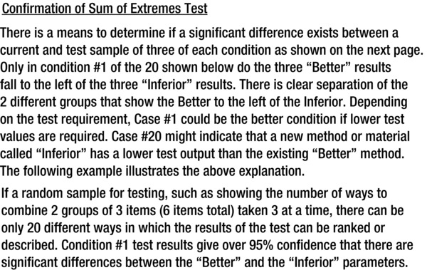
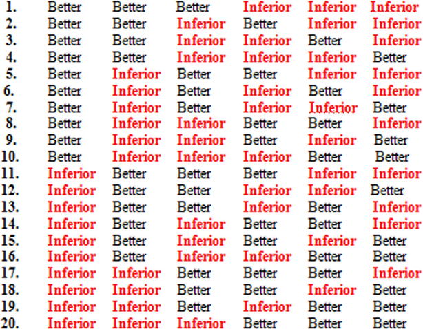
Figure E-1. Table of Possible Combinations of Two Groups of Three, Taken Six at a Time in Sum of Extremes Test
The evaluator designates the characteristic value that is to be measured and compared to a proposed replacement sample group. The “inferior” sample group represents a proposed replacement operation or a material that is being proposed to replace one that is being used. Each of the six individual samples is measured as determined by the test criteria and ranked with the results in ascending order. If the three better samples have a test score that is lower (in this case that’s good; in some tests, a higher value might be more desirable), and not tied with any of the inferior (replacement) sample scores, the data is arranged as shown in Case 1. This arrangement clearly shows that there is a significant difference in the two groups, with the better group showing lower test scores. None of the other ranked results—shown in Cases 2–20—indicate a significant difference in this same ranked relationship between the two groups with any degree of confidence. Case 1 is the only one that shows that the better group has lower-ranked values than the inferior group. (Case 20 indicates that the group classified as inferior has in this case a lower score than the better group.)
Only Condition 1 shows that all the better parts rank lower or better than and separate from the inferior rankings. Again, Condition 20 could indicate that the inferior samples are ranked below or more detrimental than the better samples. It all depends on how you set up the relationships. If only one of 20 combinations can produce the results in Condition 1, there is only a one in 20 chance that it can occur when this type of test or comparison is made.
1 / 20 = 0.05 or 5%
Consequently, if the data arranges itself in this manner after a random sample of the good and bad samples have been tested, you may be inclined to believe that there is 95% confidence that your comparison shows that a significant difference is present. But remember, even when there is 95% confidence that there is a significant difference, there is still a 5% chance that there is no significant difference, and the clue may be erroneous.
100 % – 5 % = 95 % confidence, but 100 % – 95 % = 5 % error potential
For example, consider Figure E-2. It shows the comparison of two samples of fuel pipes. The Cs indicate the brand that was being used and the Ls were a supplier’s suggested replacement part, which cost less. The comparison that was made was based on the fact that the proposed pipe had an oval shape instead of a round one. The oval pipe was greater than 0.002 inches on the L part. Consequently, the six individual components were randomized and fed into the assembly line. After assembly, they were tested for leakage. The test showed that there was clear separation of leakage provided by the two different brands. The oval pipes were detrimental. The sum of extremes in this case was six extremes, because there was clear separation of the three Cs and the three Ls, without any ties between the two groups. 3 + 3 = 6.
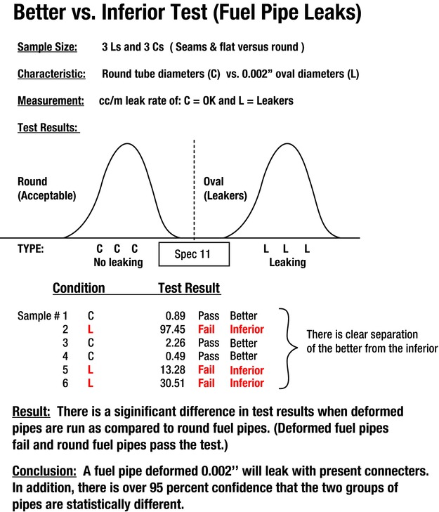
Figure E-2. Sum of Extremes Test Example (Fuel Pipe Leaks); This Is the Equivalent of Line 1 in Figure E-1
So not only can a sum of extremes comparison indicate the difference between two different conditions, samples, products, or results, it can also determine whether a change that is being considered is effective. If there is clear data separation of the groups, you have 95% confidence that the change you made is effective. 95% confidence generally provides good assurance, although you can’t establish certainty.
But again, this is only for illustrative purposes. It is better to compare five good and five bad units to generate clues or to validate that the results achieved are truly indicative of the conditions.
This last example used two groups of three, taken six at a time. Now we’ll expand that concept to the preferred method of using two groups of five, taken 10 at a time. You can develop this type of table as well. However, in the interest of space, all of the combinations are not shown here. Only ranked values that represent a statistical difference with over 95% confidence are displayed in Figure E-3. These values will still illustrate the rationale for using the recommended five acceptable and five unacceptable samples for measurement, comparison, and ranking.
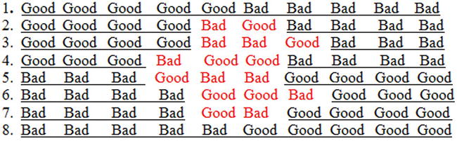
Figure E-3. Possible Combinations of Two Groups of Five, Taken 10 at a Time; They Result in a Sum of Extremes Result of Seven (7) or More
As you can see in Figure E-3, there are 252 ways that five good and five bad units of measurement can be ranked or arranged in ascending or descending order. There are only eight ways in which the ranked data can be arranged so as to create clear separation of the good and bad, with no data overlap or tied values; this method provides a sum of extremes of seven or more.1
The sum of extremes in each of these lines is 10, 8, 7, 7, 7, 7, 8, and 10. Note that 8/252 = 0.032. It is not inconsistent to say that if one of these arrangements is achieved with a comparison of five good and five bad samples (and there are at least seven qualifying extremes), then there is over 95% confidence that there is a significant difference. The different extremes are the addition of the separation of the individuals. See Examples 4 (3 good + 4 bad = 7) and 6 (4 bad + 3 good = 7). Therefore 1 – 0.032 = 0.968 or greater than 95%.
However, when you’re only visually arranging samples, there is a danger that some of the comparisons may overlap, as explained in Chapter 7. Review Figure 7-10, which is in the “Comparison of Individuals in Duos” section. It is therefore imperative that you have a measurement system in place that allows samples to be accurately ranked. Unless all the comparison values in Group 1 exceed all the comparison values in Group 2, there may be excessive overlap in the data and it may not meet the criteria of seven or more extremes. Therefore, all the comparisons of two groups of five taken two at a time must meet the seven or more extremes criteria to be meaningful.
1If you find this observation to be questionable, I invite you to determine another combination in which the observation is true. All ties between good and bad are not to be included in the sum of extremes and the sum of extremes must be 7 or more.