Chapter 6

Single-Candidate Optimization Algorithms

6.1 Optimization

We have already seen that symbolic learning by induction is a search process, where the search for the correct rule, relationship, or statement is steered by the examples that are encountered. Numerical learning systems can be viewed in the same light. An initial model is set up, and its parameters are progressively refined in the light of experience. The goal is invariably to determine the maximum or minimum value of some function of one or more variables. This is the process of optimization.

Often the optimization problem is considered to be one of determining a minimum, and the function that is being minimized is referred to as a cost function. The cost function might typically be the difference, or error, between a desired output and the actual output. Alternatively, optimization is sometimes viewed as maximizing the value of a function, known then as a fitness function. In fact, the two approaches are equivalent, because the fitness can simply be taken to be the negation of the cost and vice versa, with the optional addition of a constant value to keep both cost and fitness positive. Similarly, fitness and cost are sometimes taken as the reciprocals of each other. The term objective function embraces both fitness and cost. Optimization of the objective function might mean either minimizing the cost or maximizing the fitness.

This book focuses on stochastic, rather than deterministic methods. Deterministic methods use predictable and repeatable steps, so that the same solution is always found, provided the starting conditions are the same. For example, linear programming provides an algebraic solution to find the optimum combination of linearly scaled variables (Dantzig 1998). For more challenging searches, a computational intelligence approach is required, incorporating stochastic methods. Stochastic methods include an element of randomness that prevents guaranteed repeatability.

This chapter addresses single-candidate optimization algorithms. At all stages, there is a single trial solution that the algorithm continuously aims to improve until a stopping criterion is reached. In contrast, genetic algorithms, considered in the next chapter, maintain a population of many trial solutions.

6.2 The Search Space

The potential solutions to a search problem constitute the search space or parameter space. If a value is sought for a single variable, or parameter, the search space is one-dimensional. If simultaneous values of n variables are sought, the search space is n-dimensional. Invalid combinations of parameter values can be either explicitly excluded from the search space, or included on the assumption that they will be rejected by the optimization algorithm.

In combinatorial problems, the search space comprises combinations of values, the order of which has no particular significance, provided that the meaning of each value is known. For example, in a steel rolling mill the combination of parameters that describe the profiles of the rolls can be optimized to maximize the flatness of the manufactured steel (Nolle, Armstrong et al. 2002). Here, each possible combination of parameter values represents a point in the search space. The extent of the search space is constrained by any limits that apply to the variables.

In contrast, permutation problems involve the ordering of certain attributes. One of the best known examples is the traveling salesperson problem, where the salesperson must find the shortest route between cities of known location, visiting each city only once. This sort of problem has many real applications, such as in the routing of electrical connections on a semiconductor chip. For each permutation of cities, known as a tour, we can evaluate the cost function as the sum of distances traveled. Each possible tour represents a point in the search space. Permutation problems are often cyclic, so the tour ABCDE is considered the same as BCDEA.

The metaphor of space relies on the notion that certain points in the search space can be considered closer together than others. In the traveling salesperson example, the tour ABCDE is close to ABDCE, but DACEB is distant from both of them. This separation of patterns can be measured intuitively in terms of the number of pair-wise swaps required to turn one tour into another. In the case of binary patterns, the separation of the patterns is usually measured as the Hamming distance between them, that is, the number of bit positions that contain different values. For instance, the binary patterns 01101 and 11110 have a Hamming separation of 3.

We can associate a fitness value with each point in the search space. By plotting the fitness for a two-dimensional search space, we obtain a fitness landscape (Figure 6.1). Here, the two search parameters are x and y, constrained within a range of allowed values. For higher dimensions of search space a fitness landscape still exists, but is difficult to visualize. A suitable optimization algorithm would involve finding peaks in the fitness landscape or valleys in the cost landscape. Regardless of the number of dimensions, there is a risk of finding a local optimum rather than the global optimum for the function. A global optimum is the point in the search space with the highest fitness. A local optimum is a point whose fitness is higher than all its near neighbors but lower than that of the global optimum.

If neighboring points in the search space have a similar fitness, the landscape is said to be smooth or correlated. The fitness of any individual point in the search space is, therefore, representative of the quality of the surrounding region. Where neighboring points have very different fitnesses, the landscape is said to be rugged. Rugged landscapes typically have large numbers of local optima, and the fitness of an individual point in the search space will not necessarily reflect that of its neighbors.

The idea of a fitness landscape assumes that the function to be optimized remains constant during the optimization process. If this assumption cannot be made, as might be the case in a real-time system, we can think of the problem as finding an optimum in a fitness seascape (Mustonen and Lässig 2009, 2010).

In many problems, the search variables are not totally independent from each other. This phenomenon, in which changes in one variable lead to changes in another, is known as epistasis, and the search space is said to be epistatic.

6.3 Searching the Parameter Space

Determining the optimum for an objective function of multiple variables is not straightforward, even when the landscape is static. Although exhaustively evaluating the fitness of each point in the search space will always reveal the optimum, this is usually impracticable because of the enormity of the search space. Thus, the essence of all numerical optimization techniques is to determine the optimum point in the search space by examining only a fraction of all possible candidates.

The techniques described here are all based upon the idea of choosing a starting point and then altering one or more variables in an attempt to increase the fitness or reduce the cost. All of the methods described in this chapter maintain a single “best solution so far” that is refined until no further increase in fitness can be achieved. Genetic algorithms, which are the subject of Chapter 7, maintain a population of candidate solutions. The overall fitness of the population generally improves with each generation, although some decidedly unfit individual candidates may be added along the way.

The methods described here proceed in small steps from the start point, so each new candidate solution can never be far from the current one in the search space. The iterative improvement continues until the search reaches either the global optimum or a local optimum. To guard against missing the global optimum, it is advisable to repeat the process several times, starting from different points in the search space.

6.4 Hill-Climbing and Gradient Descent Algorithms

6.4.1 Hill-Climbing

The name hill-climbing implies that optimization is viewed as the search for a maximum in a fitness landscape. However, the method can equally be applied to a cost landscape, in which case a better name might be valley descent. It is the simplest of the optimization procedures described here. The algorithm is easy to implement, but is inefficient and offers no protection against finding a local minimum rather than the global one. From a randomly selected start point in the search space, that is, a trial solution, a step is taken in a random direction. If the fitness of the new point is greater than the previous position, it is accepted as the new trial solution. Otherwise the trial solution is unchanged. The process is repeated until the algorithm no longer accepts any steps from the trial solution. At this point the trial solution is assumed to be the optimum. As noted earlier, one way of guarding against the trap of detecting a local optimum is to repeat the process many times with different starting points.

6.4.2 Steepest Gradient Descent or Ascent

Steepest gradient descent (or ascent) is a refinement of hill climbing that can speed the convergence toward a minimum cost (or maximum fitness). It is only slightly more sophisticated than hill climbing, and it offers no protection against finding a local minimum rather than the global one. From a given starting point, that is, a trial solution, the direction of steepest descent is determined. A point lying a small distance along this direction is then taken as the new trial solution. The process is repeated until it is no longer possible to descend, at which point it is assumed that the optimum has been reached.

If the search space is not continuous but discrete—that is, it is made up of separate individual points—at each step the new trial solution is the neighbor with the highest fitness or lowest cost. The most extreme form of discrete data is where the search parameters are binary, that is, they have only two possible values. The parameters can then be placed together so that any point in the search space is represented as a binary string and neighboring points are those at a Hamming distance (see Section 6.2) of 1 from the current trial solution.

6.4.3 Gradient-Proportional Descent or Ascent

Gradient-proportional descent (or ascent), often simply called gradient descent, is a variant of steepest gradient descent that can be applied in a cost landscape that is continuous and differentiable, that is, where the variables can take any value within the allowed range and the cost varies smoothly. Rather than choosing a fixed step size, the size of the steps is allowed to vary in proportion to the local gradient of descent.

6.4.4 Conjugate Gradient Descent or Ascent

Conjugate gradient descent (or ascent) is a simple attempt at avoiding the problem of finding a local, rather than global, optimum in the cost (or fitness) landscape. From a given starting point in the cost landscape, the direction of steepest descent is initially chosen. New trial solutions are then taken by stepping along this direction, with the same direction being retained until the slope begins to curve uphill. When this happens, an alternative direction having a downhill gradient is chosen. When the direction that has been followed curves uphill, and all of the alternative directions are also uphill, it is assumed that the optimum has been reached. As the method does not continually hunt for the sharpest descent, it may be more successful than the steepest gradient descent method in finding the global minimum. However, the technique will never cause a gradient to be climbed, even though this would be necessary in order to escape a local minimum and thereby reach the global minimum.

6.4.5 Tabu Search

Tabu search is a refinement of hill-climbing methods, designed to provide some protection against becoming trapped in a local optimum (Cvijovic and Klinowski 1995; Glover and Laguna 1997). It is described by its originators as a metaheuristic algorithm, that is, it comprises some guiding rules that sit astride an existing local search method. Its key feature is a short-term memory of recent trial solutions, which are marked as “taboo” or “tabu.” These trial solutions are forbidden, which has the dual benefits, in certain circumstances, of forcing the search algorithm out of a local optimum and avoiding oscillation between alternative trial solutions. Tabu search is applicable to discrete search spaces, that is, where the search variables have discreet values, so that each candidate solution is distinct from its neighbors.

When tabu search is used alongside a standard hill-climbing algorithm, the requirement to accept new solutions only if they represent an improvement may be relaxed at heuristically determined junctures, typically when progress has stalled. Indeed, without this relaxation, previous trial solutions would be effectively taboo in any case, as they would have a lower fitness than the current trial solution. A long-term memory of the best trial solution so far would typically be used to guard against an overall deterioration of fitness.

The set of taboo solutions may be expressed in terms of complete solutions or, alternatively, as partial solutions. Partial solutions are specific attributes within a solution (e.g., a certain value for one attribute, or a particular arc in candidate circuit designs). A drawback of marking partial solutions as taboo is the risk that good complete solutions may become forbidden. This problem can be avoided by aspiration criteria, which are extra heuristics that override a trial solution’s taboo status. A typical example would be to allow a solution if it is better than the best trial solution so far, as recorded in the long-term memory.

6.5 Simulated Annealing

Simulated annealing (Kirkpatrick et al. 1983) owes its name to its similarity to the problem of atoms rearranging themselves in a cooling metal. In the cooling metal, atoms move to form a near-perfect crystal lattice, even though they may have to overcome a localized energy barrier called the activation energy, Ea, in order to do so. The atomic rearrangements within the crystal are probabilistic. The probability P of an atom jumping into a neighboring site is given by:

$P=\exp (-E_a/kT)$ (6.1)

where k is Boltzmann’s constant and T is temperature. At high temperatures, the probability approaches 1, while at T = 0 the probability is 0.

In simulated annealing, a trial solution is chosen, and the effects of taking a small random step from this position are tested. If the step results in a reduction in the cost function, it replaces the previous solution as the current trial solution. If it does not result in a cost saving, the solution still has a probability P of being accepted as the new trial solution given by:

$P=\exp (-\Delta E/T)$ (6.2)

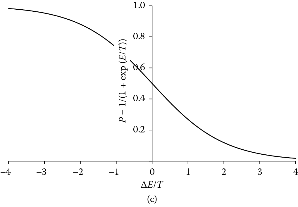
This function is shown in Figure 6.2. Here, ∆E is the increase in the cost function that would result from the step and is, therefore, analogous to the activation energy in the atomic system. There is no need to include Boltzmann’s constant, as ∆E and T no longer represent real energies or temperatures.

The temperature T is simply a numerical value that determines the stability of a trial solution. If T is high, new trial solutions will be generated continually. If T is low, the trial solution will move to a local or global cost minimum—if it is not there already—and will remain there. The value of T is initially set high and is periodically reduced according to a cooling schedule. A commonly used simple cooling schedule is:

Tt+1 = αTt (6.3)

where Tt is the temperature at step number t, and α is a constant close to, but below, 1.

While T is high, the optimization routine is free to accept many varied solutions, but as it drops, this freedom diminishes. At T = 0, the method is equivalent to the hill-climbing algorithm, as shown in Figure 6.2. So, at the start of the process, while T is high, the trial solution can roam around the whole of the search space in order to find the regions of highest fitness. This initial exploration phase is followed by exploitation as T cools, that is, a detailed search of the best region of the search space identified during exploration.

If the optimization is successful, the final solution will be the global minimum. The success of the technique is dependent upon values chosen for starting temperature, the size and frequency of the temperature decrement, and the size of perturbations applied to the trial solutions. A flowchart for the simulated annealing algorithm is given in Figure 6.3.

Johnson and Picton (Johnson and Picton 1995) have described a variant of simulated annealing in which the probability of accepting a trial solution is always probabilistic, even if it results in a decrease in the cost function (Figure 6.2). Under their scheme, the probability of accepting a trial solution is:

$P=\frac{1}{1+\exp (\Delta E/T)}$ (6.4)

where ∆E is positive if the new trial solution increases the cost function, or negative if it decreases it. In the former case P is in the range 0–0.5, and in the latter case it is in the range 0.5–1. At high temperatures, P is close to 0.5 regardless of the fitness of the new trial solution. As with standard simulated annealing, at T = 0 the method becomes equivalent to the hill-climbing algorithm, as shown in Figure 6.2.

Problems that require the optimum combination of many parameters are said to be multiobjective optimization problems. In such problems, there is a choice in the direction of the trial step in the multidimensional search space. Improved performance has been reported through the use of algorithms for selecting the step direction (Suman et al. 2010). An additional refinement is the inclusion of a variable step size. A gradual reduction in the maximum allowable step size as the iteration count rises has been shown to lead to fitter solutions in specific applications (Nolle et al. 2005).

Other modifications to simulated annealing include the use of an archive of past trial solutions, which is included alongside the current trial solution in assessing whether to jump to a new trial solution (Bandyopadhyay et al. 2008). Suman and Kumar have provided a review of some of the refinements to the basic simulated annealing algorithm (Suman and Kumar 2006).

Simulated annealing has been successfully applied to a wide variety of problems including electronic circuit design (Kirkpatrick et al. 1983), tuning specialist equipment for plasma diagnostics (Nolle, Goodyear et al. 2002), cluster analysis of weather patterns (Philipp et al. 2007), allocation of machines to manufacturing cells (Wu et al. 2008), and parameter-setting for a finisher mill in the rolling of sheet steel (Nolle, Armstrong et al. 2002).

6.6 Summary

This chapter has reviewed some numerical optimization techniques, all of which are based on minimizing a cost or maximizing a fitness. Often the cost is taken as the error between the output and the desired output. These numerical search techniques can be contrasted with a knowledge-based search. A knowledge-based system is typically used to find a path from a known, current state, such as a set of observations, to a desired state, such as an interpretation or action. In numerical optimization, we know the properties we require of a solution in terms of some fitness measure, but have no knowledge of where it lies in the search space. The problem is one of searching for locations within the search space that satisfy a fitness requirement.

All the numerical optimization techniques carry some risk of finding a local optimum rather than the global one. An attempt to overcome this is made in simulated annealing by the inclusion of an exploration phase during the early stages of the search. In these early stages, while the temperature is high, the algorithm is free to roam the search space seeking good quality regions. As the temperature cools, the algorithm migrates from exploration to exploitation, that is, seeking the peak fitness of the region that is assumed, by this stage, to contain the global optimum.

The next chapter is dedicated to a particular family of optimization algorithms that further develop the concepts of exploration and exploitation, namely genetic algorithms. Whereas all the techniques in this chapter have been based on improving a single trial solution, genetic algorithms maintain a population of trial solutions.

Further Reading

Antoniou, A., and W.-S. Lu. 2010. Practical Optimization: Algorithms and Engineering Applications. Springer, Berlin.

Marsland, S. 2009. Introduction to Machine Learning. Chapman and Hall/CRC, Boca Raton, FL.

van Laarhoven, P. J. M. 2011. Simulated Annealing: Theory and Applications. Springer, Berlin.