
Chapter 11
Systems for Interpretation and Diagnosis
11.1 Introduction
Diagnosis is the process of determining the nature of a fault or malfunction, based on a set of symptoms. Input data, that is, the symptoms, are interpreted and the underlying cause of these symptoms is the output. Diagnosis is, therefore, a special case of the more general problem of interpretation. There are many circumstances in which we may wish to interpret data, other than diagnosing problems. Examples include the interpretation of images (e.g., optical, x-ray, ultrasonic, electron microscopic), meters, gauges, and statistical data (e.g., from surveys of people or from a radiation counter). This chapter will examine some of the intelligent systems techniques that are used for diagnosis and for more general interpretation problems. The diagnosis of faults in a refrigerator will be used as an illustrative example, and the interpretation of ultrasonic images from welds in steel plates will be used as a detailed case study.
Since the inception of expert systems in the late 1960s and early 1970s, diagnosis and interpretation have been favorite application areas. Some of these early expert systems were remarkably successful and became regarded as “classics.” Three examples of these early successes are outlined as follows.
- Prospector
Prospector interpreted geological data and made recommendations of suitable sites for mineral prospecting. The system made use of Bayesian updating as a means of handling uncertainty. (See Chapter 3, Section 3.2.)
- Mycin
Mycin was a medical system for diagnosing infectious diseases and for selecting an antibiotic drug treatment. It is frequently referenced because of its novel (at the time) use of certainty theory. (See Chapter 3, Section 3.3.)
- Dendral
Dendral interpreted mass-spectrometry data, and was notable for its use of a three-phase approach to the problem:
- Phase 1: Plan
Suggest molecular substructures that may be present to guide Phase 2.
- Phase 2: Generate hypotheses
Generate all plausible molecular structures.
- Phase 3: Test
For each generated structure, compare the predicted and actual data. Reject poorly matching structures and place the remainder in rank order.
- Phase 1: Plan
A large number of intelligent systems have been produced more recently, using many different techniques, to tackle a range of diagnosis and interpretation problems in science, technology, and engineering. Rule-based diagnostic systems have been applied to power plants (Arroyo-Figueroa et al. 2000), electronic circuits (Dague et al. 1991), furnaces (Dash 1990), an oxygen generator for use on Mars (Huang et al. 1992), and batteries in the Hubble space telescope (Bykat 1990). Bayesian updating has been used in nuclear power generation (Kang and Golay 1999), while fuzzy logic has been used in automobile assembly (Lu et al. 1998) and medical data interpretation (Kumar et al. 2007). Neural networks have been used for pump diagnosis (Yamashita et al. 2000), and magnetotelluric data for geology (Manoj and Nagarajan 2003), while a neural network–rule-based system hybrid has been applied to the diagnosis of electrical discharge machines (Huang and Liao 2000).
One of the most important techniques for diagnosis is case-based reasoning (CBR), described in Chapter 5, Section 5.3. CBR has been used to diagnose cardiological diseases (Chakravarthy 2007), as well as faults in electronic circuits (Balakrishnan and Semmelbauer 1999), emergency battery backup systems (Netten 1998), and software (Hunt 1997). We will also see in this chapter the importance of models of physical systems such as power generation (Prang et al. 1996) and power distribution (Davidson et al. 2003). Applications of intelligent systems for the more general problem of interpretation include the interpretation of drawings (Maderlechner et al. 1987), seismic data (Zhang and Simaan 1987), optical spectra (Ampratwum et al. 1997), power-system alarms (Hossack et al. 2002), and nondestructive tests (Yella et al. 2006) including ultrasonic images (Hopgood et al. 1993). The last is a hybrid system, described in a detailed case study in Section 11.5.
11.2 Deduction and Abduction for Diagnosis
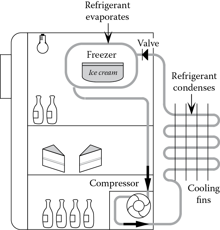
Given some information about the state of the world, we can often infer additional information. If this inference is logically correct (i.e., guaranteed to be true given that the starting information is true), then this process is termed deduction. Deduction is used to predict an effect from a given cause (see Chapter 1). Consider, for instance, a domestic refrigerator (Figure 11.1). If a refrigerator is unplugged from the electricity supply, we can confidently predict that, after a few hours, the ice in the freezer will melt, and the food in the main compartment will no longer be chilled. The new assertion (that the ice melts) follows logically from the given facts and assertions (that the power is disconnected).
Imagine that we have a frame-based representation of a refrigerator (see Chapter 4, Section 4.8), with a slot state that contains facets describing the current state of the refrigerator. If my refrigerator is represented by the frame instance my_fridge, then a simple deductive rule might be as follows, where capitalization denotes a local variable, as in Chapter 2:
rule r11_1
if state of my_fridge is unplugged
and transition_time of state of my_fridge is T
and (time_now - T) > 5 /* hours assumed */
then ice of my_fridge becomes melted
and food_temperature of my_fridge becomes ambient.
While deductive rules have an important role to play, they are inadequate on their own for problems of diagnosis and interpretation. Instead of determining an effect given a cause, diagnosis and interpretation involve finding a cause given an effect. This is termed abduction (see also Chapters 1 and 3) and involves drawing a plausible inference rather than a certain one. Thus, if we observe that the ice in our freezer has melted and the food has warmed to room temperature, we could infer from rule r11_1 that our refrigerator is unplugged. However, this is clearly an unsound inference as there may be several other reasons for the observed effects. For instance, by reference to rules r11_2 and r11_3 below, we might, respectively, infer that the fuse has blown or that there is a power blackout:
rule r11_2
if fuse of my_fridge is blown
and transition_time of fuse of my_fridge is T
and (time_now - T) > 5 /* hours assumed */
then ice of my_fridge becomes melted
and food_temperature of my_fridge becomes ambient.
rule r11_3
if power of my_fridge is blackout
and transition_time of power of my_fridge is T
and (time_now - T) > 5 /* hours assumed */
then ice of my_fridge becomes melted
and food_temperature of my_fridge becomes ambient.
So, given the observed symptoms about the temperature within the refrigerator, the cause might be that the refrigerator is unplugged, or it might be that the fuse has blown, or there might be a power blackout. Three different approaches to tackling the uncertainty of abduction are outlined in the following text: exhaustive testing, explicit modeling of uncertainty, and hypothesize-and-test.
11.2.1 Exhaustive Testing
We could use rules where the condition parts exhaustively test for every eventuality. Rules are, therefore, required of the form:
rule exhaustive
if state of my_fridge is unplugged
and transition_time of state of my_fridge is T
and (time_now - T) > 5 /* hours assumed */
and fuse of my_fridge is not blown
and power of my_fridge is not blackout
and ...
and ...
then ice of my_fridge becomes melted
and food_temperature of my_fridge becomes ambient.
This is not a practical solution, except for trivially simple domains, and the resulting rule base would be difficult to modify or maintain. In the RESCU system (Leitch et al. 1991), those rules, which can be used with confidence for both deduction and abduction, are labeled as reversible. Such rules describe a one-to-one mapping between cause and effect, such that no other causes can lead to the same effect.
11.2.2 Explicit Modeling of Uncertainty
The uncertainty can be explicitly represented using techniques such as those described in Chapter 3. This is the approach that was adopted in MYCIN and PROSPECTOR. As noted in Chapter 3, many of the techniques for representing uncertainty are founded on assumptions that are not necessarily valid.
11.2.3 Hypothesize-and-Test
A tentative hypothesis can be put forward for further investigation. The hypothesis may be subsequently confirmed or abandoned. This hypothesize-and-test approach, which was used in DENDRAL, avoids the pitfalls of finding a valid means of representing and propagating uncertainty.
There may be additional sources of uncertainty, as well as the intrinsic uncertainty associated with abduction. For example, the evidence itself may be uncertain (e.g., we may not be sure that the food isn’t cool) or vague (e.g., just what does “cool” or “chilled” mean precisely?).
The production of a hypothesis that may be subsequently accepted, refined, or rejected is similar, but not identical, to nonmonotonic logic. Under nonmonotonic logic, an earlier conclusion may be withdrawn in the light of new evidence. Conclusions that can be withdrawn in this way are termed defeasible, and a defeasible conclusion is assumed to be valid until such time as it is withdrawn.
In contrast, the hypothesize-and-test approach involves an active search for supporting evidence once a hypothesis has been drawn. If sufficient evidence is found, the hypothesis becomes held as a conclusion. If contrary evidence is found, then the hypothesis is rejected. If insufficient evidence is found, the hypothesis remains unconfirmed.
This distinction between nonmonotonic logic and the hypothesize-and-test approach can be illustrated by considering the case of our nonworking refrigerator. Suppose that the refrigerator is plugged in, the compressor is silent, and the light does not come on when the door is opened. Using the hypothesize-and-test approach, we might produce the hypothesis that there is a power blackout. We would then look for supporting evidence by testing whether another appliance is also inoperable. If this supporting evidence were found, the hypothesis would be confirmed. If other appliances were found to be working, the hypothesis would be withdrawn. Under nonmonotonic logic, reasoning would continue based on the assumption of a power blackout until the conclusion is defeated (if it is defeated at all). Confirmation is neither required nor sought in the case of nonmonotonic reasoning. Implicitly, the following default assumption is made:
rule power_assumption
if state of appliance is dead
and power is not on
/* power could be off or unknown */
then power becomes off.
/* assume for now that there is a power failure */
The term default reasoning describes this kind of implicit rule in nonmonotonic logic.
11.3 Depth of Knowledge
11.3.1 Shallow Knowledge
The early successes of diagnostic expert systems are largely attributable to the use of shallow knowledge, expressed as rules. This is the knowledge that a human expert might acquire by experience, without regard to the underlying reasons. For instance, a mechanic looking at a broken refrigerator might hypothesize that, if the refrigerator makes a humming noise but does not get cold, then it has lost coolant. While he or she may also know the detailed workings of a refrigerator, this detailed knowledge need not be used. Shallow knowledge can be easily represented:
rule r11_4
if sound of my_fridge is hum
and temperature of my_fridge is ambient
then hypothesis becomes loss_of_coolant.
Note that we are using the hypothesize-and-test approach to dealing with uncertainty in this example. With the coolant as its focus of attention, an expert system may then progress by seeking further evidence in support of its hypothesis (e.g., the presence of a leak in the pipes). Shallow knowledge is given a variety of names in the literature, including heuristic, experiential, empirical, compiled, surface, and low-road.
Expert systems built upon shallow knowledge may look impressive since they can rapidly move from a set of input data (the symptoms) to some plausible conclusions with a minimal number of intermediate steps, just as a human expert might. However, the limitations of such an expert system are easily exposed by presenting it with a situation that is outside its narrow area of expertise. When it is confronted with a set of data about which it has no explicit rules, the system cannot respond or, worse still, may give wrong answers.
There is a second important deficiency of shallow-reasoning expert systems. Because the knowledge bypasses the causal links between an observation and a deduction, the system has no understanding of its knowledge. Therefore it is unable to give helpful explanations of its reasoning. The best it can do is to regurgitate the chain of heuristic rules that led from the observations to the conclusions.
11.3.2 Deep Knowledge
Deep knowledge is the fundamental building block of understanding. A number of deep rules might make up the causal links underlying a shallow rule. For instance, the effect of the shallow rule r11_4 (above) may be achieved by the following informally stated deep rules:
rule r11_5 /* not flex format */
if current flows in the windings of the compressor
then there is an induced rotational force on the windings.
rule r11_6 /* not flex format */
if motor windings are rotating
and axle is attached to windings and compressor vanes
then compressor axle and vanes are rotating.
rule r11_7 /* not flex format */
if a part is moving
then it may vibrate or rub against its mounting.
rule r11_8 /* not flex format */
if two surfaces are vibrating or rubbing against each other
then mechanical energy is converted to heat and sound.
rule r11_9 /* not flex format */
if compressor vanes rotate
and coolant is present as a gas at the compressor inlet
then coolant is drawn through the compressor and pressurized.
rule r11_10 /* not flex format */
if pressure on a gas exceeds its vapor pressure
then the gas will condense to form a liquid.
rule r11_11 /* not flex format */
if a gas is condensing
then it will release its latent heat of vaporization.
Figure 11.2 shows how these deep rules might be used to draw the same hypothesis as the shallow rule r11_4.

There is no clear distinction between deep and shallow knowledge, but some rules are deeper than others. Thus, while rule r11_5 is deep in relation to the shallow rule r11_4, it could be considered shallow compared with knowledge of the flow of electrons in a magnetic field and the origins of the electromotive force that gives rise to the movement of the windings. In recognition of this, Fink and Lusth (Fink and Lusth 1987) distinguish fundamental knowledge, which is the deepest knowledge that has relevance to the domain. Thus, “unsupported items fall to the ground” may be considered a fundamental rule in a domain where details of Newton’s laws of gravitation are unnecessary. Similarly Kirchoff’s first law (which states that the sum of the input current is equal to the sum of the output current at any point in a circuit) would be considered a deep rule for most electrical or electronic diagnosis problems but is, nevertheless, rather shallow compared with detailed knowledge of the behavior of electrons under the influence of an electric field. Thus, Kirchoff’s first law is not fundamental in the broad domain of physics, since it can be derived from deeper knowledge. However, it may be treated as fundamental for most practical problems.
11.3.3 Combining Shallow and Deep Knowledge
There are merits and disadvantages to both deep and shallow knowledge. A system based on shallow knowledge can be very efficient, but it possesses no understanding and, therefore, has no ability to explain its reasoning. It will also fail dismally when confronted with a problem that lies beyond its expertise. The use of deep knowledge can alleviate these limitations, but the knowledge base will be much larger and less efficient. There is a trade-off between the two approaches.
The Integrated Diagnostic Model (IDM) (Fink and Lusth 1987) is a system that attempts to integrate deep and shallow knowledge. Knowledge is partitioned into deep and shallow knowledge bases, either one of which is in control at any one time. The controlling knowledge base decides which data to gather, either directly or through dialogue with the user. However, the other knowledge base remains active and is still able to make deductions. For instance, if the shallow knowledge base is in control and has determined that the light comes on when the refrigerator door is opened (as it should), the deep knowledge base can be used to deduce that the power supply is working, that the fuses are OK, that wires from power supply to bulb are OK, and that the bulb is OK. All of this knowledge then becomes available to both knowledge bases.
In IDM, the shallow knowledge base is given control first, and it passes control to the deep knowledge base if it fails to find a solution. The rationale for this is that a quick solution is worth trying first. The shallow knowledge base can be much more efficient at obtaining a solution, but it is more limited in the range of problems that it can handle. If it fails, the information that has been gathered is still of use to the deep knowledge base.
A shallow knowledge base in IDM can be expanded through experience in two ways:
- Each solved case can be stored and used to assist in solving similar cases. This is the basis of case-based reasoning (see Chapter 5).
- If a common pattern between symptom and conclusions has emerged over a large number of cases, then a new shallow rule can be created. This is an example of rule induction (see Chapter 5).
11.4 Model-Based Reasoning
11.4.1 The Limitations of Rules
The amount of knowledge about a device that can be represented in rules alone is somewhat limited. A deep understanding of how a device works—and what can go wrong with it—is facilitated by a physical model of the device being examined. Fulton and Pepe (Fulton and Pepe 1990) have highlighted three major inadequacies of a purely rule-based diagnostic system:
- Building a complete rule set is a massive task. For every possible failure, the rule-writer must predict a complete set of symptoms. In many cases, this information may not even be available because the failure may never have happened before. It may be possible to overcome the latter hurdle by deliberately causing a fault and observing the sensors. However, this is inappropriate in some circumstances, such as an overheated core in a nuclear power station.
- Symptoms are often in the form of sensor readings, and a large number of rules is needed solely to verify the sensor data (Scarl et al. 1987). Before an alarm signal can be believed at face value, related sensors must be checked to see whether they are consistent with the alarm. Without this measure, there is no reason to assume that a physical failure has occurred rather than a sensor failure.
- Even supposing that a complete rule set could be built, it would rapidly become obsolete. As there is frequently an interdependence between rules, updating the rule base may require more thought than simply adding new rules.
These difficulties can be circumvented by means of a model of the physical system. Rather than storing a huge collection of symptom–cause pairs in the form of rules, these pairs can be generated by applying physical principles to the model. The model, which is often frame-based, may describe any kind of system, including physical (Fenton et al. 2001; Wotawa 2000), software (Mateis et al. 2000), medical (Montani et al. 2003), legal (Bruninghaus and Ashley 2003), and behavioral (de Koning et al. 2000).
11.4.2 Modeling Function, Structure, and State
Practically all physical devices are made up of fundamental components such as tubes, wires, batteries, and valves. As each of these performs a fairly simple role, it also has a simple failure mode. For example, a wire may break and fail to conduct electricity, a tube can spring a leak, a battery can lose its charge, and a valve may be blocked. Given a model of how these components operate and interact to form a device, faults can be diagnosed by determining the effects of local malfunctions on the global view (i.e., on the overall device). Reasoning through consideration of the behavior of the components is sometimes termed reasoning from second principles. First principles are the basic laws of physics that determine component behavior.
Numerous different techniques and representations have been devised for modeling physical devices. Examples include the Integrated Diagnostic Model (IDM; Fink and Lusth 1987), Knowledge Engineer’s Assistant (KEATS; Motta et al. 1988), DEDALE (Dague et al. 1987), FLAME (Price 1998), NODAL (Cunningham 1998), GDE (Dekleer and Williams 1987), and ADAPtER (Portinale et al. 2004). These representations are generally based on agents, objects, or frames (see Chapter 4). ADAPtER combines elements of model-based and case-based reasoning.
The device is made up of a number of components, each of which may be represented as an instance of a class of component. The function of each component is defined within its class definition. The structure of a device is defined by links between the instances of components that make up the device. The device may be in one of several states, for example a refrigerator door may be open or closed, and the thermostat may have switched the compressor on or off. These states are defined by setting the values of instance variables.
Object-oriented programming is particularly suited to device modeling because of the clear separation of function, structure, and state. These three aspects of a device are fundamental to understanding its operation and possible malfunctions. A contrast can be drawn with mathematical modeling, where a device can often be modeled more easily by considering its overall activity than by analyzing the component processes.
Model-based reasoning can even be used to diagnose faults in computer models of physical systems, so that the diagnostic model is two layers of abstraction away from the physical world. For example, model-based reasoning has been used to diagnose faults in electronic system designs represented in VHDL (VHSIC hardware description language, where VHSIC stands for “very-high-speed integrated circuit”; Wotawa 2000). It can be regarded as a debugger for the documentation of a complex electronic system rather than a debugger for the system itself.
11.4.2.1 Function
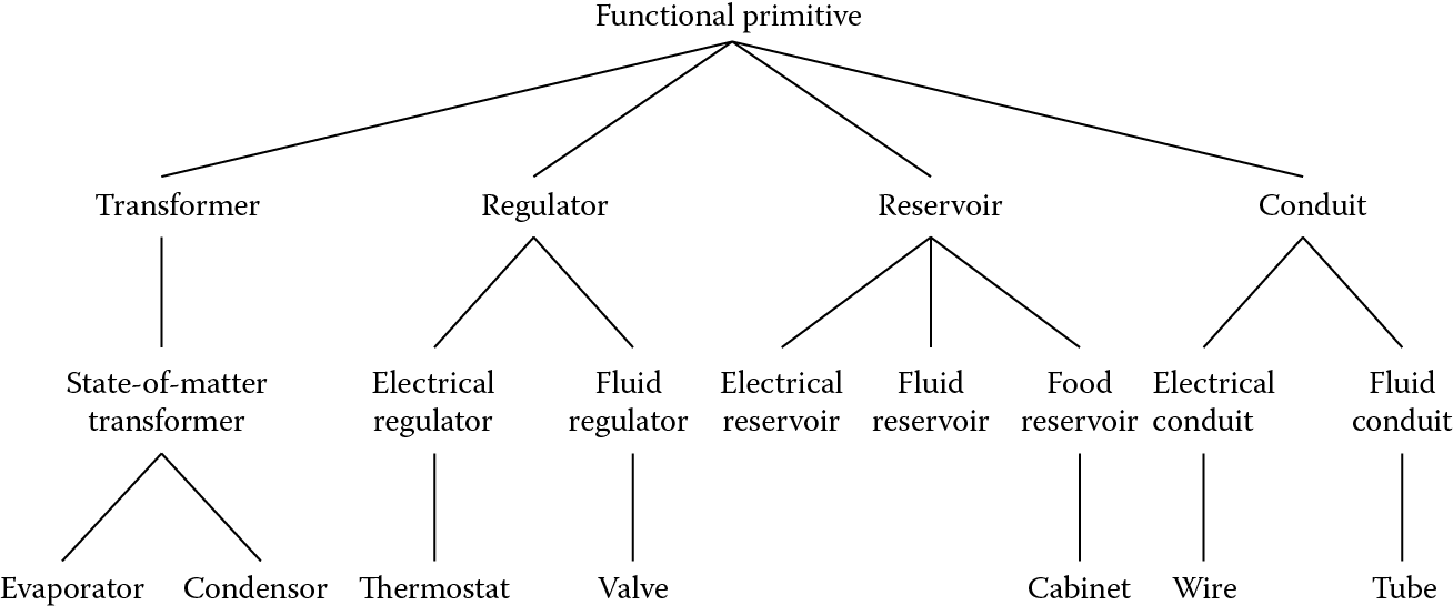
The function of a component is defined by the methods and attributes of its class. Fink and Lusth (Fink and Lusth 1987) define four functional primitives that are classes of components. All components are considered to be specializations of one of these four classes, although Fink and Lusth hint at the possible need to add further functional primitives in some applications. The four functional primitives are:
- Transformer—transforms one substance into another
- Regulator—alters the output of substance B, based upon changes in the input of substance A
- Reservoir—stores a substance for later output
- Conduit—transports substances between other functional primitives
A fifth class, sensor, may be added to this list. A sensor object simply displays the value of its input.
The word “substance” is intended to be interpreted loosely. Thus, water and electricity would both be treated as substances. The scheme was not intended to be completely general purpose, and Fink and Lusth acknowledge that it would need modifications in different domains. However, such modifications may be impractical in many domains, where specialized modeling may be more appropriate. As an illustration of the kind of modification required, Fink and Lusth point out that the behavior of an electrical conduit (a wire) is very different from a water conduit (a pipe), since a break in a wire will stop the flow of electricity, while a broken pipe will cause an out-gush of water.
These differences can be recognized by making pipes and wires specializations of the class conduit in an object-oriented representation. The pipe class requires that a substance be pushed through the conduit, whereas the wire class requires that a substance (i.e., electricity) be both pushed and pulled through the conduit. Gas pipes and water pipes would then be two of many possible specializations of the class pipe. Figure 11.3 shows a functional hierarchy of classes for some of the components of a refrigerator.
11.4.2.2 Structure
Links between component instances can be used to represent their physical associations, thereby defining the structure of a device. For example, two resistors connected in series might be represented as two instances of the class resistor and one instance of the class wire. Each instance of resistor would have a link to the instance of wire, to represent the electrical contact between them.
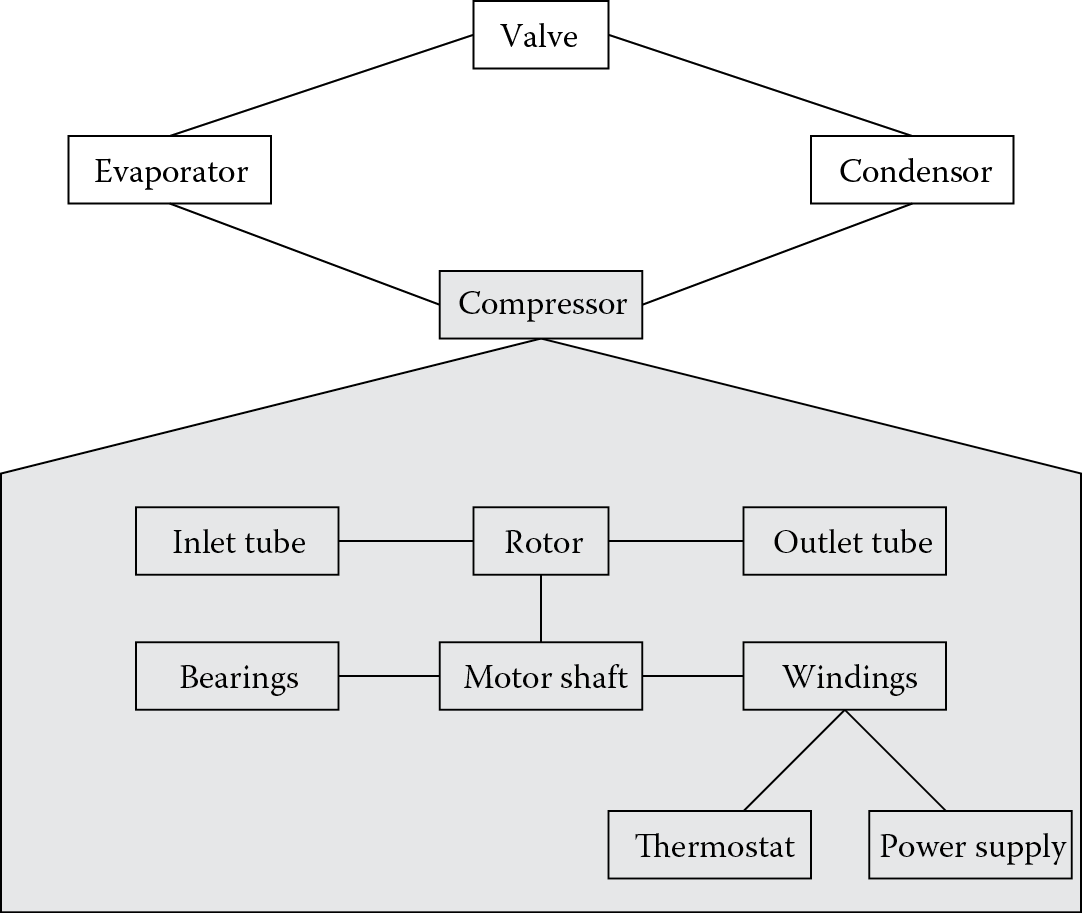
Figure 11.4 shows the instances and links that define some of the structure of a refrigerator. This figure illustrates that a compressor can be regarded either as a device made up from several components or as a component of a refrigerator. It is, therefore, an example of a functional group. The compressor forms a distinct module in the physical system. However, functional groups in general need not be modular in the physical sense. Thus, the evaporation section of the refrigerator may be regarded as a functional group even though it is not physically separate from the condensation section, and the light system forms a functional group even though the switch is physically removed from the bulb.
Many device-modeling systems can produce a graphical display of the structural layout of a device (similar to Figure 11.4), given a definition of the instances and the links between them. Some systems (e.g., KEATS and IDM) allow the reverse process as well. With these systems, the user draws a structural diagram such as Figure 11.4 on the computer screen, and the instances and links are generated automatically.
In devices where functional groups exist, the device structure is hierarchical. The hierarchical relationship can be represented by means of the composition relationship between objects (see Chapter 4). It is often adequate to consider just three levels of the structural hierarchy:
device
↓
functional group
↓
component
The application of a three-level hierarchy to the structure of a refrigerator is shown in Figure 11.5.

11.4.2.3 State
As already noted, a device may be in one of many alternative states. For example, a refrigerator door may be open or closed, and the compressor may be running or stopped. A state can be represented by setting appropriate instance variables on the components or functional groups, and transitions between states can be represented on a state map (Harel 1988) as shown in Figure 11.6 and Figure 11.7. This is an example of a finite-state machine (FSM), which is a general term for a system model based on possible states and the transitions between them. FSMs have a wide variety of applications including the design of computer games (Wagner et al. 2006).


The state of some components and functional groups will be dependent on other functional groups or on external factors. Let us consider a refrigerator that is working correctly. The compressor will be in the state running only if the thermostat is in the state closed circuit. The state of the thermostat will alter according to the cabinet temperature. The cabinet temperature is partially dependent on an external factor, namely, the room temperature, particularly if the refrigerator door is open.
The thermostat behavior can be modeled by making the attribute temperature of the cabinet object an active value (see Section 4.6.13). The thermostat object is updated every time the registered temperature alters by more than a particular amount (say, 0.5°C). A method attached to the thermostat would toggle its state between open circuit and closed circuit depending on a comparison between the registered temperature and the set temperature. If the thermostat changes its state, it would send a message to the compressor, which in turn would change its state.
A map of possible states can be drawn up, with links indicating the ways in which one state can be changed into another, that is, the transitions. A simple state map for a correctly functioning refrigerator is shown in Figure 11.6. A faulty refrigerator will have a different state map. Figure 11.7 shows the case of a thermostat that is stuck in the “open circuit” position.
Price and Hunt (Price and Hunt 1989) have modeled various mechanical devices using object-oriented programming techniques. They created an instance of the class device_state for every state of a given device. In their system, each device_state instance is made up of instance variables (e.g., recording external factors such as temperature) and links to components and functional groups that make up the device. This is sufficient information to completely restore a state. Price and Hunt found advantages in the ability to treat a device state as an object in its own right. In particular, the process of manipulating a state was simplified and kept separate from the other objects in the system. They were, thus, able to construct state maps similar to those shown in Figure 11.6 and Figure 11.7, where each state was an instance of device_state. Instance links were used to represent transitions (such as opening the door) that could take one state to another.
11.4.3 Using the Model
The details of how a model can assist the diagnostic task vary according to the specific device and the method of modeling it. In general, three potential uses can be identified:
- Monitoring the device to check for malfunctions
- Finding a suspect component, thereby forming a tentative diagnosis
- Confirming or refuting the tentative diagnosis by simulation
The diagnostic task is to determine which nonstandard component behavior in the model could make the output values of the model match those of the physical system. An overall strategy is shown in Figure 11.8. A modification of this strategy is to place a weighting on the forward links between evidence and hypotheses. As more evidence is gathered, the weightings can be updated using the techniques described in Chapter 3 for handling uncertainty. The hypothesis with the highest weighting is tried first. If it fails, the next highest is considered, and so on. The weighting may be based solely on perceived likelihood, or it may include factors such as the cost or difficulty of fixing the fault. It is often worth trying a quick and cheap repair before resorting to a more expensive solution.

When a malfunction has been detected, the single point of failure assumption is often made. This is the assumption that the malfunction has only one root cause. Such an approach is justified by Fulton and Pepe (Fulton and Pepe 1990) on the basis that no two failures are truly simultaneous. They argue that one failure will always follow the other, either independently or as a direct result.
A model can assist a diagnostic system that is confronted with a problem that lies outside its expertise. Since the function of a component is contained within the class definition, its behavior in novel circumstances may be predicted. If details of a specific type of component are lacking, comparisons can be drawn with sibling components in the class hierarchy.
11.4.4 Monitoring
A model can be used to simulate the behavior of a device. The output (e.g., data, a substance, or a signal) from one component forms the input to another component. If we alter one input to a component, the corresponding output may change, which may alter another input, and so on, resulting in a new set of sensor readings being recorded. Comparison with real world sensors provides a monitoring facility.
The RESCU system (Leitch et al. 1991) uses model-based reasoning for monitoring inaccessible plant parameters. In a chemical plant, for instance, a critical parameter to monitor might be the temperature within the reaction chamber. However, it may not be possible to measure the temperature directly, as no type of thermometer would be able to survive the highly corrosive environment. Therefore, the temperature has to be inferred from temperature measurements at the chamber walls, and from gas pressure and flow measurements.
Rules or algorithms that can translate the available measurements (Mi) into the inaccessible parameters (Pi) are described by Leitch et al. (Leitch et al. 1991) as an implicit model (Figure 11.9). Obtaining a reliable implicit model is often difficult, and model-based reasoning normally refers to the use of explicit models such as those described in Section 11.4.2. The real system and the explicit model are operated in parallel, the model generating values for the available measurements (Mi) and the inaccessible parameters (Pi). The model parameters (possibly including the parameters Pi) are adjusted to minimize the difference between the values of Mi generated by the model and the real system. This difference is called the error. By modifying the model in response to the error we have provided a feedback mechanism (Figure 11.9), discussed further in Chapter 14. This mechanism ensures that the model accurately mimics the behavior of the physical system. If a critical parameter Pi in the model deviates from its expected value, it is assumed that the same has occurred in the physical system and an alarm is triggered.
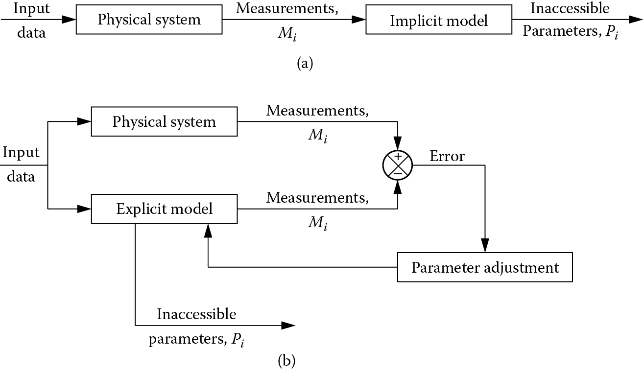
Monitoring inaccessible parameters by process modeling: (a) using an implicit model, (b) using an explicit model. (Derived from Leitch, R. et al. 1991.)
Analog devices (electrical or mechanical) can fail by varying degrees. When comparing a parameter in the physical system with the modeled value, we must decide how far apart the values have to be before we conclude that a discrepancy exists. Two ways of dealing with this problem are
- to apply a tolerance to the expected value, so that an actual value lying beyond the tolerance limit is treated as a discrepancy; and
- to give the value a degree of membership of fuzzy sets (e.g., much too high, too high, just right, and too low). The degree of membership of these fuzzy sets determines the extent of the response needed. This is the essence of fuzzy control (see Chapters 3 and 14).
It is sometimes possible to anticipate a malfunction before it actually happens. This is the approach adopted in EXPRES (Jennings 1989), a system for anticipating faults in the customer distribution part of a telephone network. The network is routinely subjected to electrical tests that measure characteristics such as resistance, capacitance, and inductance between particular points. A broken circuit, for example, would show up as a very high resistance. Failures can be anticipated and avoided by monitoring changes in the electrical characteristics with reference to the fault histories of the specific components under test and of similar components.
11.4.5 Tentative Diagnosis
The strategy for diagnosis shown in Figure 11.8 requires the generation of a hypothesis, that is, a tentative diagnosis. The method of forming a tentative diagnosis depends on the nature of the available data. In some circumstances, a complete set of symptoms and sensor measurements is immediately available, and the problem is one of interpreting them. More commonly in diagnosis, a few symptoms are immediately known and additional measurements must be taken as part of the diagnostic process. The tentative diagnosis is a best guess, or hypothesis, of the actual cause of the observed symptoms. We will now consider three ways of generating a tentative diagnosis.
11.4.5.1 The Shotgun Approach
Fulton and Pepe (Fulton and Pepe 1990) advocate collecting a list of all objects that are upstream of the unexpected sensor reading. All of these objects are initially under suspicion. If several sensors have recorded unexpected measurements, only one sensor need be considered as it is assumed that there is only one cause of the problem. The process initially involves diagnosis at the functional grouping level. Identification of the faulty functional group may be sufficient, in which case the diagnosis can stop and the functional group can simply be replaced in the real system. Alternatively, the process may be repeated by examining individual components within the failed functional group to locate the failed component.
11.4.5.2 Structural Isolation
KEATS (Motta et al. 1988) has been used for diagnosing faults in analog electronic circuits, and makes use of the binary chop or structural isolation strategy of Milne (Milne 1987). Initially the electrical signal is sampled in the middle of the signal chain and compared with the value predicted by the model. If the two values correspond, then the fault must be downstream of the sampling point, and a measurement is then taken halfway downstream. Conversely, if there is a discrepancy between the expected and actual values, the measurement is taken halfway upstream. This process is repeated until the defective functional grouping has been isolated. If the circuit layout permits, the process can be repeated within the functional grouping in order to isolate a specific component. Motta et al. found in their experiments that the structural isolation strategy closely resembles the approach adopted by human experts (Motta et al. 1988). They have also pointed out that the technique can be made more sophisticated by modifying the binary chop strategy to reflect heuristics concerning the most likely location of the fault.
11.4.5.3 The Heuristic Approach
Either of the preceding two strategies can be refined by the application of shallow (heuristic) knowledge. As noted previously, IDM (Fink and Lusth 1987) has two knowledge bases, containing deep and shallow knowledge. If the shallow knowledge base has failed to find a quick solution, the deep knowledge base seeks a tentative solution using a set of five guiding heuristics:
- If an output from a functional unit is unknown, find out its value by testing or by interaction with a human operator.
- If an output from a functional unit appears incorrect, check its input.
- If an input to a functional unit appears incorrect, check the source of the input.
- If the input to a functional unit appears correct but the output is not, assume that the functional unit is faulty.
- Examine components that are nodes before those that are conduits, as the former are more likely to fail in service.
11.4.6 Fault Simulation
Both the correct and the malfunctioning behavior of a device can be simulated using a model. The correct behavior is simulated during the monitoring of a device (Section 11.4.4). Simulation of a malfunction is used to confirm or refute a tentative diagnosis. A model allows the effects of changes in a device or in its input data to be tested. A diagnosis can be tested by changing the behavior of the suspected component within the model and checking that the model produces the symptoms that are observed in the real system. Such tests cannot be conclusive, as other faults might also be capable of producing the same symptoms, as noted in Section 11.2. Suppose that a real refrigerator is not working and makes no noise. If the thermostat on the refrigerator is suspected of being permanently open-circuit, this malfunction can be incorporated into the model and the effects noted. The model would show the same symptoms that are observed in the real system. The hypothesis is then confirmed as the most likely diagnosis.
Most device simulations proceed in a step-by-step manner, where the output of one component (component A) becomes the input of another (component B). Component A can be thought of as being “upstream” of component B. An input is initially supplied to the components that are furthest upstream. For instance, the thermostat is given a cabinet temperature, and the power cord is given a simulated supply of electricity. These components produce outputs that become the inputs to other components, and so on. This sort of simulation can run into difficulties if the model includes a feedback loop. In these circumstances, a defective component not only produces an unexpected output, but also has an unexpected input. The output can be predicted only if the input is known, and the input can be predicted only if the output is known. One approach to this problem is to supply initially all of the components with their correct input values. If the defective behavior of the feedback component is modeled, its output and input values would be expected to converge on a failure value after a number of iterations. Fink and Lusth (Fink and Lusth 1987) found that convergence was achieved in all of their tests, but they acknowledge that there might be cases where this does not happen.
11.4.7 Fault Repair
Once a fault has been diagnosed, the next step is normally to fix the fault. Most fault diagnosis systems offer some advice on how a fault should be fixed. In many cases this recommendation is trivial, given the diagnosis. For example, the diagnosis worn bearings might be accompanied by the recommendation replace worn bearings, while the diagnosis leaking pipe might lead to the recommendation fix leak. A successful repair provides definite confirmation of a diagnosis. If a repair fails to cure a problem, then the diagnostic process must recommence. A failed repair may not mean that a diagnosis was incorrect. It is possible that the fault that has now been fixed has caused a second fault that also needs to be diagnosed and repaired.
11.4.8 Using Problem Trees
Some researchers (Dash 1990; Steels 1989) favor the explicit modeling of faults, rather than inferring faults from a model of the physical system. Dash (Dash 1990) builds a hierarchical tree of possible faults (a problem tree, see Figure 11.10), similar to those used for classifying case histories (Figure 5.3). Unlike case-based reasoning, problem trees cover all anticipated faults, whether or not they have occurred previously. By applying deep or shallow rules to the observed symptoms, progress can be made from the root (a general problem description) to the leaves of the tree (a specific diagnosis). The tree is, therefore, used as a means of steering the search for a diagnosis. An advantage of this approach is that a partial solution is formed at each stage in the reasoning process. A partial solution is generated even if there is insufficient knowledge or data to produce a complete diagnosis.

11.4.9 Summary of Model-Based Reasoning
Some of the advantages of model-based reasoning are listed as follows:
- A model is less cumbersome to maintain than a rule base. Real-world changes are easily reflected in changes in the model.
- The model need not waste effort looking for sensor verification. Sensors are treated identically to other components, and therefore a faulty sensor is as likely to be detected as any other fault.
- Unusual failures are just as easy to diagnose as common ones. This is not the case in a rule-based system, which is likely to be most comprehensive in the case of common faults.
- The separation of function, structure, and state may help a diagnostic system to reason about a problem that is outside its area of expertise.
- The model can simulate a physical system, for the purpose of monitoring or for verifying a hypothesis.
Model-based reasoning only works well in situations where there is a complete and accurate model. It is inappropriate for physical systems that are too complex to model properly, such as medical diagnosis or weather forecasting. An ideal would be to build a model for monitoring and diagnosis directly from CAD data generated during the design stage. The model would then be available as soon as a device entered service.
11.5 Case Study: A Blackboard System for Interpreting Ultrasonic Images
One of the aims of this book is to demonstrate the application of a variety of techniques, including knowledge-based systems, computational intelligence, and procedural computation. The more complicated problems have many facets, where each facet may be best suited to a different technique. This is true of the interpretation of ultrasonic images, which will be discussed as a case study in the remainder of this chapter. A blackboard system has been used to tackle this complex interpretation problem (Hopgood et al. 1993). As we saw in Chapter 9, blackboard systems allow a problem to be divided into subtasks, each of which can be tackled using the most suitable technique.
An image interpretation system attempts to understand the processed image and describe the world represented by it. This requires symbolic reasoning (using rules, objects, relationships, list-processing, or other techniques) as well as numerical processing of signals (Walker and Fox 1987). ARBS (Algorithmic and Rule-based Blackboard System) (Hopgood et al. 1998) and its successor DARBS (Distributed ARBS) (Tait et al. 2008; Nolle et al. 2001) have been designed to incorporate both types of processes. Numerically intensive signal processing, which may involve a large amount of raw data, is performed by conventionally coded agents. Facts, causal relationships, and strategic knowledge are symbolically encoded in one or more knowledge bases. This explicit representation allows encoded domain knowledge to be modified or extended easily. Signal processing routines are used to transform the raw data into a description of its key features (i.e., into a symbolic image) and knowledge-based techniques are used to interpret this symbolic image.
The architecture allows signal interpretation to proceed opportunistically, building up from initial subsets of the data through to higher-level observations and deductions. When a particular set of rules needs access to a chunk of raw data, it can have it. No attempt has been made to write rules that look at the whole of the raw data, as the preprocessing agents avoid the need for this. Although a user interface is provided to allow monitoring and intervention, DARBS is designed to run independently, producing a log of its actions and decisions.
11.5.1 Ultrasonic Imaging
Ultrasonic imaging is widely used for the detection and characterization of features, particularly defects, in manufactured components. The technique belongs to a family of nondestructive testing methods that are distinguished by the ability to examine components without causing any damage. Various arrangements can be used for producing ultrasonic images. Typically, a transmitter and receiver of ultrasound (i.e., high frequency sound at approximately 1–10 MHz) are situated within a single probe that makes contact with the surface of the component. The probe emits a short pulse of ultrasound and then detects waves returning as a result of interactions with the features within the specimen. If the detected waves are assumed to have been produced by single reflections, then the time of arrival can be readily converted to the depth (z) of these features. By moving the probe in one dimension (y), an image can be plotted of y versus z, with intensity often represented by color or grayscale. This image is called a b-scan, and it approximates to a cross-section through a component. It is common to perform such scans with several probes pointing at different angles into the specimen, and to collect several b-scans by moving the probes in a raster (Figure 11.11).

A typical b-scan image is shown in Figure 11.12. A threshold has been applied, so that only received signals of intensity greater than −30 db are displayed, and these appear as black dots on the image. Ten probes were used, pointing into the specimen at five different angles. Because ultrasonic beams are not collimated, a point defect is detected over a range of y values, giving rise to a characteristic arc of dots on the b-scan image. Arcs produced by a single probe generally lie parallel to each other and normal to the probe direction. The point of intersection of arcs produced by different probes is a good estimate of the location of the defect that caused them.
The problems of interpreting a b-scan are different from those of other forms of image interpretation. The key reason for this is that a b-scan is not a direct representation of the inside of a component, but rather it represents a set of wave interactions (reflection, refraction, diffraction, interference, and mode conversion) that can be used to infer some of the internal structure of the component.
11.5.2 Agents in DARBS
Each agent in DARBS is an autonomous parallel process. The agents can run concurrently on one computer or distributed across many computers connected by the Internet. Each agent is represented as a structure comprising seven primary elements, shown in Figure 11.13. The latest open-source version of DARBS* represents all agents, rules, messages, and blackboard information in XML (Extensible Markup Language). XML is a standard format for textual information, widely used for Web documents but equally appropriate for structuring the textual information used in DARBS.

The first element of an agent specifies its name and the second specifies its type. For rule-based agents, the third and fourth elements specify the inference mode and rules, respectively. An activation flag in the fifth element allows individual agents to be switched on or off. The sixth element contains a set of preconditions that must be satisfied before the agent performs a task. Each agent constantly monitors the blackboard, waiting for its preconditions to be satisfied so that it can become active. As soon as the preconditions are satisfied, the agent performs its task opportunistically. Unlike earlier blackboard implementations, such as ARBS, there is no need for a scheduler in DARBS. The precondition may comprise subconditions joined with Boolean operators and and or. Finally, the seventh element states what actions are to be performed before the agent finishes its task. For procedural, neural network and other non rule-based agents, the functions and procedures are listed in the action element.
Agents in DARBS can read data from the blackboard simultaneously. However, to avoid deadlock, only one agent is allowed to write data to the same partition of the blackboard at one time. Whenever the content of the blackboard changes, the blackboard server broadcasts a message to all agents. The agents themselves decide how to react to this change; for example, it may be appropriate for an agent to restart its current task. With this approach, agents are completely opportunistic, that is, activating themselves whenever they have some contributions to make to the blackboard.
When an agent is active, it applies its knowledge to the current state of the blackboard, adding to it or modifying it. If an agent is rule-based, then it is essentially a rule-based system in its own right. A rule’s conditions are examined and, if they are satisfied by a statement on the blackboard, the rule fires and the actions dictated by its conclusion are carried out. Single or multiple instantiation of variables can be selected. When the rules are exhausted, the agent is deactivated and any actions in the actions element are performed. These actions usually involve reports to the user or the addition of control information to the blackboard. If the agent is procedural or contains a neural network or genetic algorithm, then the required code is simply included in the actions element and the elements relating to rules are ignored.
The blackboard architecture is able to bring together the most appropriate tools for handling specific tasks. Procedural tasks are not entirely confined to procedural agents, since rules within a rule-based agent can access procedural code from either their condition or conclusion parts. In the case of ultrasonic image interpretation, procedural agents written in C++ are used for fast, numerically intensive data-processing. An example is the procedure that preprocesses the image, using the Hough Transform to detect lines of indications (or dots). Rule-based agents are used to represent specialist knowledge, such as the recognition of image artifacts caused by probe reverberations. Neural network agents can be used for judgmental tasks, such as classification, that involve the weighing of evidence from various sources. Judgmental ability is often difficult to express in rules, and neural networks were incorporated into DARBS as a response to this difficulty.
11.5.3 Rules in DARBS
Rules are used in DARBS in two contexts:
- to express domain knowledge within a rule-based agent and
- to express the applicability of an agent through its preconditions.
Just as agents are activated in response to information on the blackboard, so too are individual rules within a rule-based agent. The main functions of DARBS rules are to look up information on the blackboard, to draw inferences from that information, and to post new information on the blackboard. Rules can access procedural code for performing such tasks as numerical calculations or database lookup.
In early versions of DARBS, rules were implemented as lists (see Chapter 10, Section 10.2.1), delineated by square brackets. These have subsequently been replaced by XML structures. The rules are interpreted by sending them to a parser, that is, a piece of software that breaks down a rule into its constituent parts and interprets them. The DARBS rule parser first extracts the condition statement and evaluates it, using recursion if there are embedded subconditions. If a rule is selected for firing and its overall condition is found to be true, all of the conclusion statements are interpreted and carried out.
Atomic conditions (i.e., conditions that contain no subconditions) can be evaluated in any of the following ways:
- Test for the presence of information on the blackboard, and look up the information if it is present.
- Call algorithms or external procedures that return Boolean or numerical results.
- Numerically compare variables, constants, or algorithm results.
The conclusions, or subconclusions, can comprise any of the following:
- Add or remove information to or from the blackboard.
- Call an algorithm or external procedure, and optionally add the results to the blackboard.
- Report actions to the operator.
The strategy for applying rules is a key decision in the design of a system. In many types of rule-based system, this decision is irrevocable, committing the rule-writer to either a forward-chaining or backward-chaining system. However, the blackboard architecture allows much greater flexibility, as each rule-based agent can use whichever inference mechanism is most appropriate. The rule structure has been designed so flexibly that fuzzy rules can be incorporated without changing either the rule syntax or inference engines (Hopgood et al. 1998).
DARBS offers a choice of inference engines, including options for multiple and single instantiation of variables, described in Chapter 2, Section 2.7.1. Under multiple instantiation, all possible matches to the variables are found and acted upon with a single firing of a rule. In contrast, only the first match to the variables is found when single instantiation is used (Hopgood 1994). Figure 11.14 shows the difference between the two inference engines in the case of a rule that analyses rectangular areas of arc intersection in the image.

Firing a rule using: (a) multiple instantiation of variables and (b) single instantiation of variables.
The hybrid inference mechanism described in Chapter 2, Section 2.10 requires the construction of a network representing the dependencies between the rules. A separate dependence network can be built for each rule-based agent, prior to running the system. The networks are saved and only need to be regenerated if the rules are altered. The code to generate the networks is simplified by the fact that the only interaction between rules is via the blackboard. For rule A to enable rule B to fire, rule A must either add something to the blackboard that rule B needs to find or it must remove something that rule B requires to be absent. When a rule-based agent is activated, the rules within the agent are selected for examination in the order dictated by the dependence network.
Rule-based agents in DARBS can generate hypotheses that can then be tested and thereby supported, confirmed, weakened, or refuted. DARBS uses this hypothesize-and-test approach (see Section 11.2.3) to handle the uncertainty that is inherent in problems of abduction and the uncertainty that arises from sparse or noisy data. The hypothesize-and-test method reduces the solution search space by focusing attention on those agents relevant to the current hypothesis.
11.5.4 The Stages of Image Interpretation
The problem of ultrasonic image interpretation can be divided into three distinct stages: arc detection, gathering information about the regions of intersecting arcs, and classifying defects on the basis of the gathered information. These stages are now described in more detail.
11.5.4.1 Arc Detection Using the Hough Transform
The first step toward defect characterization is to place on the blackboard the important features of the image. This is achieved by a procedural agent that examines the image (Figure 11.15) and fits arcs to the data points (Figure 11.15). In order to produce these arcs, a Hough transform (Duda and Hart 1972) is used to determine the groupings of points. The transform has been modified so that isolated points some distance from the others are not included. The actual positions of the arcs are determined by least squares fitting.
(a) 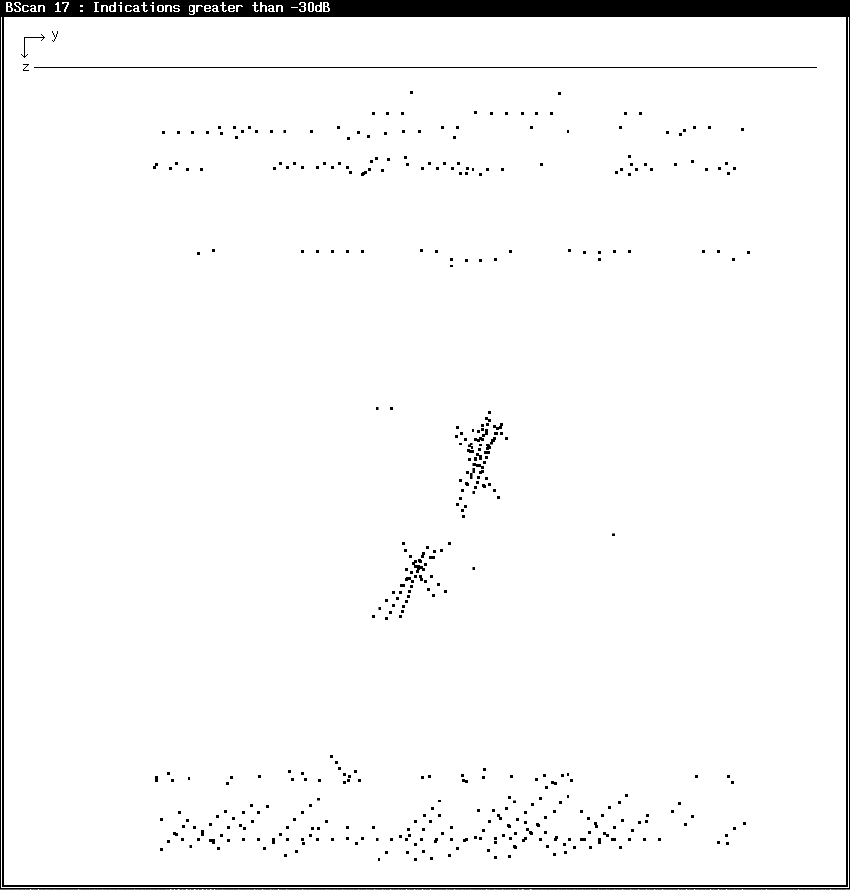
(b) 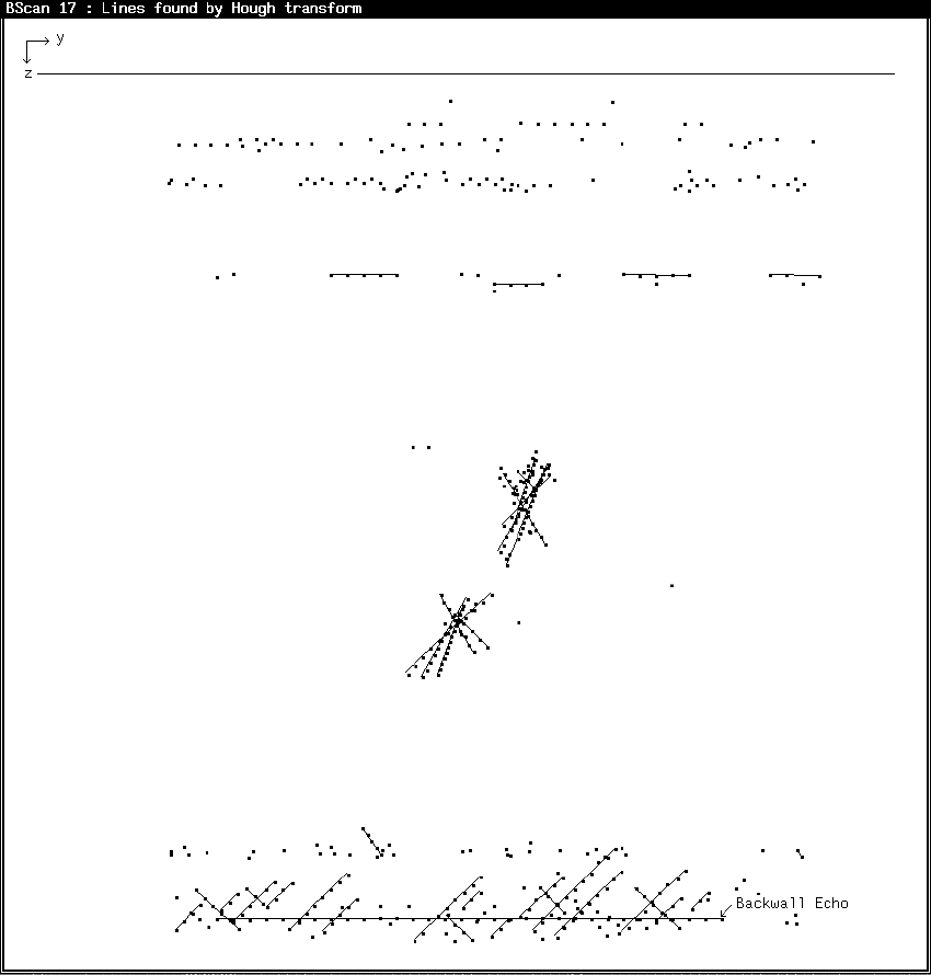
The stages of interpretation of a b-scan image: (a) before interpretation and (b) with lines found by a Hough transform.
This preprocessing phase is desirable in order to reduce the volume of data and to convert it into a form suitable for knowledge-based interpretation. Thus, knowledge-based processing begins on data concerning approximately 30 linear arcs rather than on data concerning 400–500 data points. No information is lost permanently. If, in the course of its operations, DARBS judges that more data concerning a particular line would help the interpretation, it retrieves the information about the individual points that compose that line and represents these point data on the blackboard. It is natural, moreover, to work with lines rather than points in the initial stages of interpretation. Arcs of indications are produced by all defect types, and much of the knowledge used to identify flaws is readily couched in terms of the properties of lines and the relations between them.
11.5.4.2 Gathering the Evidence
Once a description of the lines has been recorded on the blackboard, a rule-based agent picks out those lines that are considered significant according to criteria such as intensity, number of points, and length. Rules are also used to recognize the back wall echo and lines that are due to probe reverberation. Both are considered “insignificant” for the time being. Key areas in the image are generated by finding points of intersection between significant lines and then grouping them together. Figure 11.15 shows the key areas found by applying this method to the lines shown in Figure 11.15. For large smooth cracks, each of the crack tips is associated with a distinct area. Other defects are entirely contained in their respective areas.
Rule-based agents are used to gather evidence about each of the key areas. The evidence includes:
- Size of the area
- Number of arcs passing through it
- Shape of the echodynamic (defined in the following text)
- Intensity of indications
- Sensitivity of the intensity to the angle of the probe
The echodynamic associated with a defect is the profile of the signal intensity along one of the “significant” lines. This is of considerable importance in defect classification as different profiles are associated with different types of defects. In particular, the echodynamics for a smooth crack face, a spheroidal defect (e.g., a single pore or an inclusion) or crack tip, and a series of gas pores are expected to be similar to those in Figure 11.16 (Halmshaw 1987). In DARBS, pattern classification of the echodynamic is performed using a fast Fourier transform and a set of rules to analyze the features of the transformed signal. A neural network has also been used for the same task (see Section 11.5.5).
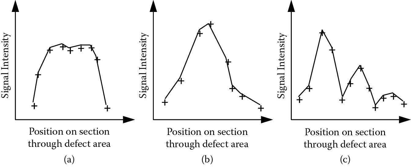
Echodynamics across (a) a crack face, (b) a crack tip, pore, or inclusion, and (c) an area of porosity.
The sensitivity of the defect to the angle of the probe is another critical indicator of the nature of the defect in question. Roughly spherical flaws, such as individual gas pores, have much the same appearance when viewed from different angles. Smooth cracks on the other hand have a much more markedly directional character—a small difference in the direction of the probe may result in a considerable reduction (or increase) in the intensity of indications. The directional sensitivity of an area of intersection is a measure of this directionality and is represented in DARBS as a number between −1 and 1.
11.5.4.3 Defect Classification
Quantitative evidence about key areas in an image is derived by rule-based agents, as described earlier. Each piece of evidence provides clues as to the nature of the defect associated with the key area. For instance, the indications from smooth cracks tend to be sensitive to the angle of the probe, and the echodynamic tends to be plateau-shaped. In contrast, indications from a small round defect (e.g., an inclusion) tend to be insensitive to probe direction and have a cusp-shaped echodynamic. There are several factors like these that need to be taken into account when producing a classification, and each must be weighted appropriately.
Two techniques for classifying defects based upon the evidence have been tried using DARBS: a rule-based hypothesize-and-test approach and a neural network. In the former approach, hypotheses concerning defects are added to the blackboard. These hypotheses relate to smooth or rough cracks, porosity, or inclusions. They are tested by deriving from them expectations (or predictions) relating to other features of the image. On the basis of the correspondence between the expectations and the image, DARBS arrives at a conclusion about the nature of a defect, or, where this is not possible with any degree of certainty, it alerts the user to a particular problem case.
Writing rules to verify the hypothesized defect classifications is a difficult task and, in practice, the rules need continual refinement and adjustment in the light of experience. The use of neural networks to combine the evidence and produce a classification provides a means of circumventing this difficulty since they need only a representative training set of examples, instead of the formulation of explicit rules.
11.5.5 The Use of Neural Networks
Neural networks have been used in DARBS for two quite distinct tasks, described in the following text.
11.5.5.1 Defect Classification Using a Neural Network
Neural networks can perform defect classification, provided there are sufficient training examples and the evidence can be presented in numerical form. In this study (Hopgood et al. 1993), there were insufficient data to train a neural network to perform a four-way classification of defect types, as done under the hypothesize-and-test method. Instead, a backpropagation network was trained to classify defects as either critical (i.e., a smooth crack) or noncritical on the basis of four local factors: the size of the area, the number of arcs passing through it, the shape of the echodynamic, and the sensitivity of the intensity to the angle of the probe. Each of these local factors was expressed as a number between −1 and 1.
Figure 11.17 shows plots of evidence for the 20 defects that were used to train and test a neural network. The data are, in fact, points in four-dimensional space, where each dimension represents one of the four factors considered. Notice that the clusters of critical and noncritical samples might not be linearly separable. This means that traditional numerical techniques for finding linear discriminators (Duda and Hart 1973) are not powerful enough to produce good classification. However, a multilayer perceptron (MLP, see Chapter 8) is able to discriminate between the two cases, since it is able to find the three-dimensional surface required to separate them. Using the leave-one-out technique (Chapter 8, Section 8.4.6), an MLP with two hidden layers correctly classified 16 out of 20 images from defective components (Hopgood et al. 1993).


11.5.5.2 Echodynamic Classification Using a Neural Network
One of the inputs to the classification network requires a value between −1 and 1 to represent the shape of the echodynamic. This value can be obtained by using a rule-based agent that examines the Fourier components of the echodynamic and uses heuristics to provide a numerical value for the shape. An alternative approach is to use another neural network to generate this number.
An echodynamic is a signal intensity profile across a defect area and can be classified as a cusp, plateau, or wiggle. Ideally, a neural network would make a three-way classification, given an input vector derived from the amplitude components of the first n Fourier coefficients, where 2n is the echodynamic sample rate. However, cusps and plateaux are difficult to distinguish since they have similar Fourier components, so a two-way classification is more practical, with cusps and plateaux grouped together. A multilayer perceptron has been used for this purpose.
11.5.5.3 Combining the Two Applications of Neural Networks
The use of two separate neural networks in distinct agents for the classification of echodynamics and of the potential defect areas might seem unnecessary. Because the output of the former feeds, via the blackboard, into the input layer of the latter, this arrangement is equivalent to a hierarchical MLP (Chapter 8, Section 8.4.4). In principle, the two networks could have been combined into one large neural network, thereby removing the need for a preclassified set of echodynamics for training. However, such an approach would lead to a loss of modularity and explanation facilities. Furthermore, it may be easier to train several small neural networks separately on subtasks of the whole classification problem than to attempt the whole problem at once with a single large network. These are important considerations when there are many subtasks amenable to connectionist treatment.
11.5.6 Rules for Verifying Neural Networks
Defect classification, whether performed by the hypothesize-and-test method or by neural networks, has so far been discussed purely in terms of evidence gathered from the region of the image that is under scrutiny. However, there are other features in the image that can be brought to bear on the problem. Knowledge of these features can be expressed easily in rule form and can be used to verify the classification. The concept of the use of rules to verify the outputs from neural networks was introduced in Chapter 9, Section 9.5. In this case, an easily identifiable feature of a b-scan image is the line of indications due to the back wall echo. A defect in the sample, particularly a smooth crack, will tend to cast a “shadow” on the back wall directly beneath it (Figure 11.18). The presence of a shadow in the expected position can be used to verify the location and classification of a defect. In this application, the absence of this additional evidence is not considered a strong enough reason to reject a defect classification. Instead, the classification in such cases is marked for the attention of a human operator, as there are grounds for doubt over its accuracy.

11.6 Summary
This chapter has introduced some of the techniques that can be used to tackle the problems of automated interpretation and diagnosis. Diagnosis is considered to be a specialized case of the more general problem of interpretation. It has been shown that a key part of diagnosis and interpretation is abduction, the process of determining a cause, given a set of observations. There is uncertainty associated with abduction, since causes other than the selected one might give rise to the same set of observations. Two possible approaches to dealing with this uncertainty are to explicitly represent the uncertainty using the techniques described in Chapter 3, or to hypothesize-and-test. As the name implies, the latter technique involves generating a hypothesis (or best guess), and either confirming or refuting the hypothesis depending on whether it is found to be consistent with the observations.
Several different forms of knowledge can contribute to a solution. We have paid specific attention to rules, case histories, and physical models. We have also shown that neural networks and conventional programming can play important roles when included as part of a blackboard system. Rules can be used to represent both shallow (heuristic) and deep knowledge. They can also be used for the generation and verification of hypotheses. Case-based reasoning, introduced in Chapter 5, involves comparison of a given scenario with previous examples and their solutions. Model-based reasoning relies on the existence of a model of the physical system, where that model can be used for monitoring, generation of hypotheses, and verification of hypotheses by simulation.
Blackboard systems have been introduced as part of a case study into the interpretation of ultrasonic images. These systems allow various forms of knowledge representation to come together in one system. They are, therefore, well suited to problems that can be broken down into subtasks. The most suitable form of knowledge representation for different subtasks is not necessarily the same, but each subtask can be individually represented by a separate intelligent agent.
A neural network agent was shown to be effective for combining evidence generated by other agents and for categorizing the shape of an echodynamic. This approach can be contrasted with the use of a neural network alone for interpreting images. The blackboard architecture avoids the need to abandon rules in favor of neural networks or vice versa, since the advantages of each can be incorporated into a single system. Rules can represent knowledge explicitly, whereas neural networks can be used where explicit knowledge is hard to obtain. Although neural networks can be rather impenetrable to the user and are unable to explain their reasoning, these deficiencies can be reduced by using them for small-scale localized tasks with reports generated in between.
Further Reading
Ding, S. X. 2008. Model-based Fault Diagnosis Techniques: Design Schemes, Algorithms, and Tools. Springer, Berlin.
Korbicz, J., J. M. Koscielny, Z. Kowalczuk, and W. Cholewa, eds. 2004. Fault Diagnosis: Models, Artificial Intelligence, Applications. Springer, Berlin.
Price, C. J. 2000. Computer-Based Diagnostic Systems. Springer Verlag, Berlin.