Chapter 8
Neural Networks
8.1 Introduction
Artificial neural networks are a family of techniques for numerical learning, like the optimization algorithms reviewed in Chapters 6 and 7, but in contrast to the symbolic learning techniques reviewed in Chapter 5. They consist of many nonlinear computational elements that form the network nodes or neurons, linked by weighted interconnections. They are analogous in structure to the neurological system in humans and animals, which is made up of real rather than artificial neural networks. Practical artificial neural networks are much simpler than biological ones, so it is unrealistic to expect them to produce the sophisticated behavior of humans or animals. Nevertheless, they are effective at a range of tasks based on pattern matching. Throughout the rest of this book we will use the expression neural network to mean an artificial neural network. The technique of using neural networks is described as connectionism.
Each node in a neural network may have several inputs, each of which has an associated weighting. The node performs a simple computation on its input values, which are single integers or real numbers, to produce a single numerical value as its output. The output from a node can either form an input to other nodes or be part of the output from the network as a whole. The overall effect is that a neural network generates a pattern of numbers at its outputs in response to a pattern of numbers at its inputs. These patterns of numbers are one-dimensional arrays known as vectors, for example, (0.1, 1.0, 0.2).
Each neuron performs its computation independently of the other neurons, except that the outputs from some neurons may form the inputs to others. Thus, neural networks have a highly parallel structure that allows them to take advantage of parallel processing computers. They can also run on conventional serial computers—they just take longer to run that way. Neural networks are tolerant of the failure of individual neurons or interconnections. The performance of the network is said to degrade gracefully if these localized failures within the network should occur.
The weights on the node interconnections, together with the overall topology, define the output vector that is derived by the network from a given input vector. The weights do not need to be known in advance, but can be learned by adjusting them automatically using a training algorithm. In the case of supervised learning, the weights are derived by repeatedly presenting to the network a set of example input vectors along with the corresponding desired output vector for each of them. The weights are adjusted with each iteration until the actual output for each input is close to the desired vector. In the case of unsupervised learning, the examples are presented without any corresponding desired output vectors. With a suitable training algorithm, the network adjusts its weights in accordance with naturally occurring patterns in the data. The output vector then represents the position of the input vector within the discovered patterns of the data.
Part of the appeal of neural networks is that, when presented with noisy or incomplete data, they will produce an approximate answer rather than one that is incorrect. This is another aspect of the graceful degradation of neural networks mentioned earlier. Similarly, when presented with unfamiliar data that lie within the range of its previously seen examples, the network will generally produce an output that is a reasonable interpolation between the example outputs. Neural networks are, however, unable to extrapolate reliably beyond the range of the previously seen examples. Interpolation can also be achieved by fuzzy logic (see Chapter 3). Thus, neural networks and fuzzy logic often represent alternative solutions to a particular engineering problem and may be combined in a hybrid system (see Chapter 9).
8.2 Neural Network Applications
Neural networks can be applied to a diversity of tasks, but they all have the common theme of pattern recognition. In general, the network associates a pattern in the form of an input vector (x1, x2, … xn) with a particular output vector (y1, y2, … ym), although the function linking the two may be unknown and may be highly nonlinear. (A linear function is one that can be represented as f(x) = ax + c, where a and c are constants; a nonlinear one may include higher order terms for x, or trigonometric or logarithmic functions of x.)
8.2.1 Classification
Often the output vector from a neural network is used to represent one of a set of known possible outcomes, that is, the network acts as a classifier. For example, a speech recognition system could be devised to recognize three different words: yes, no, and maybe. The digitized sound of the words would be preprocessed in some way to form the input vector. The desired output vector would then be either (0, 0, 1), (0, 1, 0), or (1, 0, 0), representing the three classes of the words.
Such a network would be trained using a set of examples known as the training data. Each example would comprise a digitized utterance of one of the words as the input vector, using a range of different voices, together with the corresponding desired output vector. During training, the network learns to associate similar input vectors with a particular output vector. When it is subsequently presented with a previously unseen input vector, the network selects the output vector that offers the closest match. This type of classification would not be straightforward using nonconnectionist techniques, as the input data rarely correspond exactly to any one example in the training data.
8.2.2 Nonlinear Estimation
Neural networks provide a useful technique for determining the values of variables that cannot be measured easily, but which are known to depend in some complex way on other more accessible variables. The measurable variables form the network input vector and the unknown variables constitute the output vector. We can call this use nonlinear estimation. The network is initially trained using a set of examples that comprise the training data. Supervised learning is used, so each example in the training comprises two vectors: an input vector and its corresponding desired output vector. (This assumes that some values for the less accessible variable have been obtained to form the desired outputs.) During training, the network learns to associate the example input vectors with their desired output vectors. When it is subsequently presented with a previously unseen input vector, the network is able to interpolate between similar examples in the training data to generate an output vector.
8.2.3 Clustering
Clustering is a form of unsupervised learning, that is, the training data comprises a set of example input vectors without any corresponding desired output vectors. As successive input vectors are presented, they are clustered into N groups, where the integer N may be prespecified or may be allowed to grow according to the diversity of the data. For instance, digitized preprocessed spoken words could be presented to the network. The network would learn to cluster together the examples that it considered to be in some sense similar to each other. In this example, the clusters might correspond to different words or different voices.
Once the clusters have formed, a second neural network can be trained to associate each cluster with a particular desired output. The overall system then becomes a classifier, where the first network is unsupervised and the second one is supervised. Clustering is useful for data compression and is an important aspect of data mining, that is, finding patterns in complex data.
8.2.4 Content-Addressable Memory
The use of a neural network as a content-addressable memory involves a form of supervised learning. During training, each example input vector becomes stored in a dispersed form through the network. There are no separate desired output vectors associated with the training data, as the training data represent both the inputs and the desired outputs.
When a previously unseen vector is subsequently presented to the network, it is treated as though it were an incomplete or error-ridden version of one of the stored examples. So the network regenerates the stored example that most closely resembles the presented vector. This application can be thought of as a type of classification, where each of the examples in the training data belongs to a separate class, and each represents the ideal vector for that class. This approach is useful when classes can be characterized by an ideal or perfect example. For example, printed text that is subsequently scanned to form a digitized image will contain noisy and imperfect examples of printed characters. For a given font, an ideal version of each character can be stored in a content-addressable memory and produced as its output whenever an imperfect scanned version is presented as its input. Thus, a form of automatic character recognition is achieved.
8.3 Nodes and Interconnections
Each node, or neuron, in a neural network is a simple computing element having an input side and an output side. Each node may have directional connections to many other nodes at both its input and output sides. Each input xi is multiplied by its associated weight wi. Typically, the node’s role is to sum each of its weighted inputs and add a bias term w0 to form an intermediate quantity called the activation, a. It then passes the activation through a nonlinear function ft known as the transfer function or activation function. Figure 8.1 shows the function of a single neuron.

The behavior of a neural network depends on its topology, the weights, the bias terms, and the transfer function. The weights and biases can be learned, and the learning behavior of a network depends on the chosen training algorithm. Typically a sigmoid function is used as the transfer function, as shown in Figure 8.2. The sigmoid function (von Seggern 2007) is given by:


Nonlinear transfer functions: (a) a sigmoid function; (b) a ramp function; (c) a step function.
(8.1)
For a single neuron, the activation a is given by:
(8.2)
where n is the number of inputs, and the bias term w0 is defined separately for each node. Figures 8.2(b) and (c) show the ramp and step functions, which are alternative nonlinear functions sometimes used as transfer functions.
Many network topologies are possible, but we will concentrate on a selection that illustrates some of the different applications for neural networks. We will start by looking at single and multilayer perceptrons, which can be used for classification or, more generally, for nonlinear mapping. We will then consider the category of recurrent networks, which are used for tasks that include classification of data with a temporal context and acting as a content-addressable memory. The final category, unsupervised networks, is all used for clustering.
8.4 Single and Multilayer Perceptrons
8.4.1 Network Topology
The topology of a multilayer perceptron (MLP) is shown in Figure 8.3. The neurons are organized in layers, such that each neuron is totally connected to the neurons in the layers above and below, but not to the neurons in the same layer. These networks are also called feedforward networks, although this term could be applied more generally to any network where the direction of data flow is always “forward,” that is, toward the output. MLPs can be used either for classification or as nonlinear estimators. The number of nodes in each layer and the number of layers are determined by the network builder, often on a trial-and-error basis.

There is always an input layer and an output layer; the number of nodes in each is determined by the number of inputs and outputs being considered. There may be any number of layers between these two layers. Unlike the input and output layers, the layers in between often have no obvious meaning associated with them, and they are known as hidden layers. If there are no hidden layers, the network is a single layer perceptron (SLP). The network shown in Figure 8.3 has three input nodes, two hidden layers with four nodes each and an output layer of two nodes. It can, therefore, be described as a 3–4–4–2 MLP.
An MLP operates by feeding data forward along the interconnections from the input layer, through the hidden layers, to the output layer. With the exception of the nodes in the input layer, the inputs to a node are the outputs from each node in the previous layer. At each node apart from those in the input layer, the data are weighted, summed, added to the bias, and then passed through the transfer function.
There is some inconsistency in the literature over the counting of layers, arising from the fact that the input nodes do not perform any processing, but simply feed the input data into the nodes above. Thus although the network in Figure 8.3 is clearly a four-layer network, it only has three processing layers. An SLP has two layers (the input and output layers) but only one processing layer, namely the output layer.
8.4.2 Perceptrons as Classifiers
In general, neural networks are designed so that there is one input node for each element of the input vector and one output node for each element of the output vector. Thus, in a classification application, each output node would usually represent a particular class. A typical representation for a class would be for a value close to 1 to appear at the corresponding output node, with the remaining output nodes generating a value close to 0. A simple decision rule is needed in conjunction with the network, for example, the “winner takes all” rule selects the class corresponding to the node with the highest output. If the input vector does not fall into any of the classes, none of the output values may be very high. For this reason, a more sophisticated decision rule might be used, for example, one that specifies that the output from the winning node must also exceed a predetermined threshold such as 0.5.
Instead of having one output node per class, more compact representations are also possible for classification problems. Hallam et al. have used just two output nodes to represent four classes (Hallam et al. 1990). This was achieved by treating both outputs together, so that the four possibilities corresponding to four classes are (0,0), (0,1), (1,0), and (1,1). One drawback of this approach is that it is more difficult to interpret an output that does not closely match one of these possibilities (e.g., what would an output of [0.5, 0.5] represent?).
Let us now return to the more usual case where each output node represents a distinct class. Consider the practical example of an MLP for interpreting satellite images of the Earth in order to recognize different forms of land use (Hopgood 2005). Figure 8.4 shows a region of the Mississippi Delta, imaged at six different wavebands. The 6–10–5 MLP shown in Figure 8.5 was trained to associate the six waveband images with the corresponding land use. The pixels of the waveband images constitute the inputs and the five categories of land use (water, trees, cultivated, soil/rock, swamp) constitute the outputs. The network was trained pixel-by-pixel on just the top 1/16 of these images and tested against the whole images, 15/16 of which were previously unseen. The results are shown in Figure 8.6. The classification is mostly correct, although some differences between the results and the actual land use can be seen. The neural network performance could certainly be improved with a little refinement, but it has deliberately been left unrefined so that these discrepancies can be seen. Nevertheless, the network’s ability to generalize from a limited set of examples is clearly demonstrated.
(a) 
(b) 
(c)
(d) 
(e) 
(f) 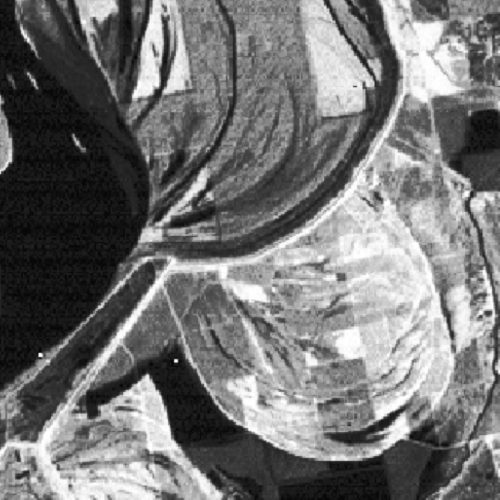
Portion of a Landsat-4™ satellite image of an area just to the south of Memphis, Tennessee, taken in six different wavebands. (Source: NASA.)


Classification results: (a) actual land use map; (b) portion used for training; (c) land use map from neural network outputs. (Derived from Hopgood 2005.)
In the preceding example, each input vector has six elements, so it can be represented as a point in six-dimensional state space, sometimes called the pattern space. Six dimensions are hard to visualize but, if the input vector has only two elements, it can be represented as a point in two-dimensional state space. The process of classification is then one of drawing dividing lines between regions. A single layer perceptron, with two neurons in the input layer and the same number of neurons in the output layer as there are classes, can associate with each class a single straight dividing line, as shown in Figure 8.7. Classes that can be separated in this way are said to be linearly separable. More generally, n-dimensional input vectors are points in n-dimensional hyperspace. If the classes can be separated by (n–1)-dimensional hyperplanes, they are linearly separable.

Dividing up the pattern space: (a) linearly separable classes; (b) nonlinearly separable classes. Data points belonging to classes 1, 2, and 3 are, respectively, represented by ◾ , ⦁, and +.
To see how an SLP divides up the pattern space with hyperplanes, consider a single processing neuron of an SLP. Its output, prior to application of the transfer function, is a real number given by Equation 8.2. Regions of the pattern space that clearly belong to the class represented by the neuron will produce a strong positive value, and regions that clearly do not belong to the class will produce a strong negative value. The classification becomes increasingly uncertain as the activation a becomes close to zero, and the dividing criterion is usually assumed to be a = 0. This would correspond to an output of 0.5 after the application of the sigmoid transfer function (Figure 8.2). Thus, the hyperplane that separates the two regions is given by:
(8.3)
In the case of two inputs, Equation 8.3 becomes simply the equation of a straight line, since it can be rearranged as:
(8.4)
where −w1/w2 is the gradient and −w0/w2 is the intercept on the x2 axis.
For problems that are not linearly separable, as in Figure 8.7, regions of arbitrary complexity can be drawn in the state space by a multilayer perceptron with one hidden layer and a differentiable, that is, smooth, transfer function such as the sigmoid function (Figure 8.2). The first processing layer of the MLP can be thought of as dividing up the state space with straight lines (or hyperplanes), and the second processing layer forms multifaceted regions by Boolean combinations (and, or, and not) of the linearly separated regions. It is therefore generally accepted that only one hidden layer is necessary to perform any nonlinear mapping or classification with an MLP that uses a sigmoid transfer function (Figure 8.8). This is Kolmogorov’s Existence Theorem (Hornick et al. 1989). Similarly, no more than two hidden layers are required if a step transfer function is used. However, the ability to learn from a set of examples cannot be guaranteed and, therefore, the detailed topology of a network inevitably involves a certain amount of trial and error. A pragmatic approach to network design is to start with a small network and expand the number of nodes or layers as necessary.
(a) 
(b) 
(c) 
(d) 
Regions in state space distinguished by a perceptron. (Derived from Rumelhart et al. 1986b.) A convex region has the property that a line joining points on the boundary passes only through that region. (a) No hidden layers: region is a half plane bounded by a hyperplane; (b) one hidden layer with step transfer function: convex open region; (c) one hidden layer with step transfer function: convex closed region; (d) two hidden layers with step transfer function; or one hidden layer with smooth transfer function. Regions of arbitrary complexity can be defined.
8.4.3 Training a Perceptron
During training, a multilayer perceptron learns to separate the regions in state space by adjusting its weights and bias terms. Appropriate values are learned from a set of examples comprising input vectors and their corresponding desired output vectors. An input vector is applied to the input layer, and the output vector produced at the output layer is compared with the desired output. For each neuron in the output layer, the difference between the generated value and the desired value is the error. The overall error for the neural network is expressed as the square root of the mean of the squares of the errors. This is the root-mean-squared (RMS) value, designed to take equal account of both negative and positive errors. The RMS error is minimized by altering the weights and bias terms, which may take many passes through the training data. The search for the combination of weights and biases that produces the minimum RMS error is an optimization problem like those considered in Chapter 7, where the cost function is the RMS error. When the RMS error has become acceptably low for each example vector, the network is said to have converged, and the weights and bias terms are retained for application of the network to new input data.
One of the most commonly used training algorithms is the back-error propagation algorithm, sometimes called the generalized delta rule (Rumelhart et al. 1986a, 1986b). This is a gradient-proportional descent technique (see Chapter 7), and it relies upon the transfer function being continuous and differentiable. The sigmoid function (Figure 8.2) is a particularly suitable choice, as will be shown in the following, because its derivative ft′(a) is simply given by:
(8.5)
Remember that ft(a) is the output y from a neuron when the transfer function ft is applied to its activation a.
The use of the back-error propagation algorithm for optimizing weights and bias terms can be made clearer by treating the biases as weights on the interconnections from dummy nodes, whose output is always 1, as shown in Figure 8.9. A flowchart describing the back-error propagation algorithm is presented in Figure 8.10, using the nomenclature shown in Figure 8.9.

Nomenclature for the back-error propagation algorithm in Figure 8.7 . N L = number of layers (4 in this example). w Aij = weight between node i on level A and node j on level A –1 (N L ≥ A ≥ 2). a Ai = activation at node i on level A. y Ai = output from node i on level A. δ Ai = an error term associated with node i on level A.

At the core of the algorithm is the delta rule that determines the modifications to the weights, ∆wBij:
(8.6)
for all nodes j in layer A and all nodes i in layer B, where A = B − 1. Neurons in the output layer and in the hidden layers have an associated error term, δ (pronounced delta). When the sigmoid transfer function is used, δAj is given by:
(8.7)
The learning rate, η, is applied to the calculated values for δAj. Knight (Knight 1990) suggests a value for η of about 0.35. As written in Equation 8.6, the delta rule includes a momentum coefficient, α, although this term is sometimes omitted, that is, α is sometimes set to zero. Gradient-proportional descent techniques can be inefficient, especially close to a minimum in the cost function, which in this case is the RMS error of the output. To address this, a momentum term forces changes in weight to be dependent on previous weight changes. The value of the momentum coefficient must be in the range 0–1. Knight suggests that α be set to 0.0 for the first few training passes and then increased to 0.9 (Knight 1990).
Other training algorithms have also been successfully applied to perceptrons. For instance, Willis et al. (1991) favor the chemotaxis algorithm, which incorporates a random statistical element in a similar fashion to simulated annealing (see Chapter 6, Section 6.5). Other alternative learning algorithms have been developed, for example (Campolucci et al. 1997; Moallem and Monadjemi 2010), but the backpropagation algorithm remains the most widely used approach.
8.4.4 Hierarchical Perceptrons
In complex problems involving many inputs, some researchers recommend dividing an MLP into several smaller MLPs arranged in a hierarchy, as shown in Figure 8.11. In this example, the hierarchy comprises two levels. The inputs are shared among the MLPs at level 1, and the outputs from these networks form the inputs to an MLP at level 2. This approach is often useful if meaningful intermediate variables can be identified as the outputs from the level 1 MLPs. For example, if the inputs are measurements from sensors for monitoring equipment, the level 1 outputs could represent diagnosis of any faults, and the level 2 outputs could represent the recommended control actions (Kim and Park 1993). In this example, a single large MLP could, in principle, be used to map directly from the sensor measurements to the recommended control actions. However, convergence of the smaller networks in the hierarchical MLP is likely to be achieved more easily. Furthermore, as the constituent networks in the hierarchical MLP are independent from each other, they can be trained either separately or in parallel.

8.4.5 Buffered Perceptrons
Many forms of classification require contextual information, that is, information that either precedes or follows the example being classified. Examples include weather forecasting, where an individual air pressure reading is much more meaningful in the context of whether it is increasing or decreasing, or at a peak or minimum. Similarly, neural networks for classifying speech require contextual information for individual words, and for syllables within words. Neural networks that take account of such time-dependent effects are said to be dynamic.
The family of recurrent neural networks (Section 8.5) is specifically designed to be dynamic. One approach to providing contextual information with an MLP is to provide a buffer as part of the input layer. At any one time, the input to the MLP comprises the current input values plus their context, that is, their values at the previous and subsequent time step. At the next time step, all inputs are advanced so that the input at time t becomes part of the context for the input at time t+1. This approach was used in the NETtalk system for converting written text to speech (Sejnowski and Rosenberg 1986).
8.4.6 Some Practical Considerations
Sometimes it is appropriate to stop the training process before the point where no further reductions in the RMS error are possible. This is because it is possible to over-train the network, so that it becomes expert at giving the correct output for the training data, but less expert at dealing with new data. This is likely to be a problem if the network has been trained for too many cycles or if the network is over-complex for the task in hand. For instance, the inclusion of additional hidden layers or large numbers of neurons within the hidden layers will tend to promote over-training. The effect of over-training is shown in Figure 8.12 for a nonlinear mapping of a single input parameter onto a single output parameter, and Figure 8.12 shows the effect of over-training using the nonlinearly separable classification data from Figure 8.7.
(a) 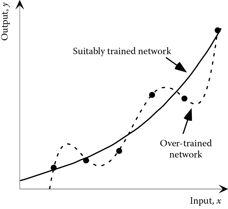
(b) 
The effect of over-training: (a) nonlinear estimation; (b) classification (⦁, ◾, and + are data points used for training)
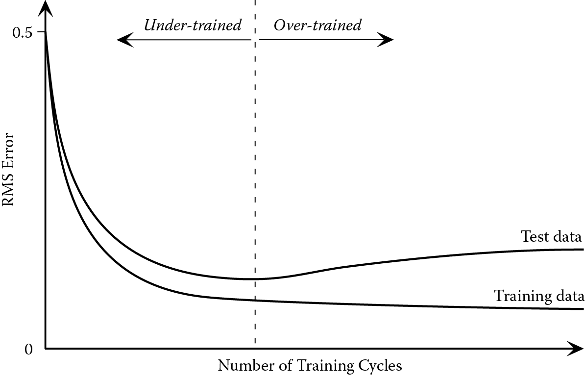
One way of avoiding over-training is to divide the data into three sets, known as the training, testing, and validation data. Training takes place using the training data, and the RMS error with these data is monitored. However, at predetermined intervals the training is paused and the current weights saved. At these points, before training resumes, the network is presented with the test data and an RMS error calculated. The RMS error for the training data decreases steadily until it stabilizes. However, the RMS error for the test data may pass through a minimum and then start to increase again because of the effect of over-training, as shown in Figure 8.13. As soon as the RMS error for the test data starts to increase, the network is over-trained, but the previously stored set of weights would be close to the optimum. Finally, the performance of the network can be evaluated by testing it using the previously unseen validation data.
A problem that is frequently encountered in real applications is a shortage of suitable data for training and testing a neural network. Hopgood et al. (Hopgood et al. 1993) describe a classification problem where there were only 20 suitable examples, which needed to be shared between the training and testing data. They used a technique called leave-one-out as a way of reducing the effect of this problem. The technique involves repeatedly training on all but one of the examples and testing on the missing one. So, in this case, the network would initially be trained on 19 of the examples and tested on the remaining one. This procedure is repeated a further 19 times, omitting a different example each time from the training data, resetting the weights to random values, retraining, and then testing on the omitted example. The leave-one-out technique is clearly time-consuming, as it involves resetting the weights, training, testing, and scoring the network many times, that is, 20 times in this example. Its advantage is that the performance of the network can be evaluated using every available example as though it were previously unseen test data.
Neural networks that accept real numbers are only effective if the input values are constrained to suitable ranges, typically between 0 and 1 or between −1 and 1. The range of the outputs depends on the chosen transfer function, for example, the output range is between 0 and 1 if the sigmoid function is used. In real applications, the actual input and output values may fall outside these ranges or may be constrained to a narrow band within them. In either case the data will need to be scaled, usually linearly, before being presented to the neural network. Some neural network packages perform the scaling automatically.
8.5 Recurrent Networks
8.5.1 Simple Recurrent Network (SRN)
The buffered perceptrons, considered in Section 8.4.5, provide temporal context for a particular set of inputs. However, they do so at a cost, as this approach significantly increases the number of connections and requires a prior knowledge of the number of preceding and subsequent inputs that are required to provide the context. In order to reduce the need for an external buffer, several recurrent neural network architectures have been developed. Their distinctive feature is that they contain connections that feedback from the processing layers of the network (i.e., the hidden and/or output layers) to the input layer. These connections can be used to present to the network the recent input history, as the context for the current input.
The classic format is the simple recurrent network (SRN), developed by Elman (Elman 1991). The SRN is based on a three-layer perceptron, with additional feedback connections from the hidden layer to the input, as shown in Figure 8.14. These feedback connections link to additional input nodes, whose function is to provide a context, or immediate history, for the current inputs. The initial activations of the context neurons are set to zero, corresponding to an output of 0.5 if the sigmoid transfer function is used. Subsequently, the outputs of the context neurons at time t are copies of the outputs from the hidden layer neurons at time t−1. All of the feedback connections must, therefore, have weights equal to 1. As each hidden neuron connects to one context neuron, the SRN must contain the same number of context neurons as hidden neurons.

Training of the SRN proceeds in the same manner as an MLP, using the back-error propagation algorithm to adjust the weights on the feedforward connections, while the weights on the feedback connections are left set to 1. The training algorithm adjusts the weights on the connections into the hidden layer to produce the correct context for the next pattern in the sequence. It simultaneously adjusts the weights on the connections into the output layer to produce the desired output for the current input pattern.
SRNs have been applied to various time-dependent processing applications such as the generation of facial expression for robots (Matsui et al. 2009; Matsui et al. 2008) and modeling the intracranial pressure for patients in neurosurgical intensive care (Shieh et al. 2004). However, the majority of applications have concerned the understanding and generation of natural language (Cernanský et al. 2007; Chalup and Blair 2003; Frank 2006).
A major drawback with the SRN is that it can only take account of historical context. In the case of natural language and speech processing, this means that the network can take into account the prior utterances, but not the subsequent ones. This weakness was addressed in an alternative architecture called STORM (Spatio Temporal Self-Organizing Recurrent Map) that provides both forward and backward context to a self-organizing map (or SOM, described in Section 8.6.2; McQueen et al. 2005).
8.5.2 Hopfield Network
The Hopfield network has only one layer, and the nodes are used for both input and output. The network topology is shown in Figure 8.15. The network is normally used as a content-addressable memory where each training example is treated as a model vector or exemplar, to be stored by the network. The Hopfield network uses binary input values, typically 1 and −1. By using the step nonlinearity shown in Figure 8.2 as the transfer function ft, the output is forced to remain binary, too. If the activation a is 0, that is, on the step, the output is indeterminate, so a convention is needed to yield an output of either 1 or −1.


The topology of: (a) the Hopfield network, (b) the MAXNET. Circular connections from a node to itself are allowed in the MAXNET, but are disallowed in the Hopfield network.
If the network has Nn nodes, then the input and output would both comprise a vector of Nn binary digits. If there are Ne exemplars to be stored, the network weights and biases are set according to the following equations:
(8.8)
(8.9)
where wij is the weighting on the connection from node i to node j, wi0 is the bias on node i, and xik is the ith digit of example k. There are no circular connections from a node to itself, hence wij = 0 where i = j.
Setting weights in this way constitutes the learning phase, and results in the exemplars being stored in a distributed fashion in the network. If a new vector is subsequently presented as the input, then this vector is initially the output, too, as nodes are used for both input and output. The node function (Figure 8.1) is then performed on each node in parallel. If this is repeated many times, the output will be progressively modified and will converge on the exemplar that most closely resembles the initial input vector. In order to store reliably at least half the exemplars, Hopfield estimated that the number of exemplars (Ne) should not exceed approximately 0.15Nn (Hopfield 1982).
If the network is to be used for classification, a further stage is needed in which the result is compared with the exemplars to pick out the one that matches.
8.5.3 MAXNET
The MAXNET (Figure 8.15) has an identical topology to the Hopfield network, except that the weights on the circular interconnections, wii, are not always zero as they are in the Hopfield network. The MAXNET is used to recognize which of its inputs has the highest value. In this role it is sometimes used in conjunction with other networks, such as a multilayer perceptron, to select the output node that generates the highest value. Suppose that the multilayer perceptron has four output nodes, corresponding to four different categories. A MAXNET to determine the maximum output value (and, hence, the solution to the classification task) would have four nodes and four alternative output patterns after convergence, that is, four exemplars:
|
x |
0 |
0 |
0 |
|
0 |
x |
0 |
0 |
|
0 |
0 |
x |
0 |
|
0 |
0 |
0 |
x |
where x > 0. The MAXNET would adjust its highest input value to x, and reduce the others to 0. Note that the MAXNET is constructed to have the same number of nodes (Nn) as the number of exemplars (Ne). Contrast this with the Hopfield network, which needs approximately seven times as many nodes as exemplars.
Using the same notation as Equations 8.8 and 8.9, interconnection weights are set as follows:
(8.10)
8.5.4 The Hamming Network
The Hamming network has two parts—a twin layered feedforward network and a MAXNET, as shown in Figure 8.16. The feedforward network is used to compare the input vector with each of the examples, awarding a matching score to each example. The MAXNET is then used to pick out the example that has attained the highest score. The overall effect is that the network can categorize its input vector.

8.6 Unsupervised Networks
8.6.1 Adaptive Resonance Theory (ART) Networks
All of the neural networks introduced so far have used supervised learning, that is, the network has been shown the desired output, and it learns by minimizing the error in relation to the desired outputs. The Adaptive Resonance Theory networks (ART1 and ART2) of Carpenter and Grossberg (Carpenter and Grossberg 1987) are worthy of mention because they are early examples of networks that learn without supervision. The ART1 network topology comprises bidirectional interconnections between a set of input nodes and a MAXNET, as shown in Figure 8.17.

The network classifies the incoming data into clusters. When the first example is presented to the network, it becomes stored as an exemplar or model pattern. The second example is then compared with the exemplar and is either considered sufficiently similar to belong to the same cluster or stored as a new exemplar. If an example is considered to belong to a previously defined cluster, the exemplar for that cluster is modified to take account of the new member. The performance of the network is dependent on the way in which the differences are measured, that is, the closeness measure, and the threshold or vigilance, ρ, beyond which a new exemplar is stored. As each new vector is presented, it is compared with all of the current exemplars in parallel. The number of exemplars grows as the network is used, that is, the network learns new patterns. The operation of the ART1 network, which takes binary inputs, is summarized in Figure 8.18. ART2 is similar but takes continuously varying inputs.

8.6.2 Kohonen Self-Organizing Networks
Kohonen self-organizing networks, sometimes called self-organizing maps (SOMs), provide another example of networks that can learn without supervision. The processing nodes can be imagined to be arranged in a two-dimensional array, known as the Kohonen layer (Figure 8.19). There is also a separate one-dimensional layer of input nodes, where each input node is connected to each node in the Kohonen layer. As in the MLP, the input neurons perform no processing but simply pass their input values to the processing neurons, with an applied weighting.

As in the ART networks, the Kohonen network learns to cluster together similar patterns. The learning mechanism involves competition between the neurons to respond to a particular input vector (Kohonen 1987, 1988; Hecht-Nielson 1990; Lippmann 1987). The “winner” has its weightings set so as to generate a high output, approaching 1. The weightings on nearby neurons are also adjusted so as to produce a high value, but the weights on the “losers” are left alone. The neurons that are nearby the winner constitute a neighborhood.
When the trained network is presented with an input pattern, one neuron in the Kohonen layer will produce an output larger than the others, and is said to have fired. When a second similar pattern is presented, the same neuron or one in its neighborhood will fire. As similar patterns cause topologically close neurons to fire, clustering of similar patterns is achieved. The effect can be demonstrated by training the network using pairs of Cartesian coordinates. The trained network has the property that the distribution of the firing neurons corresponds with the Cartesian coordinates represented by the input vector. Thus, if the input elements fall in the range between −1 and 1, then an input vector of (−0.9, 0.9) will cause a neuron close to one corner of the Kohonen layer to fire, while an input vector of (0.9, −0.9) would cause a neuron close to the opposite corner to fire.
Although Kohonen self-organizing networks are unsupervised, they can form part of a hybrid network for supervised learning. This is achieved by passing the coordinates of the firing neuron to an MLP. In this arrangement, learning takes place in two distinct phases. First, the Kohonen self-organizing network learns, without supervision, to associate regions in the pattern space with clusters of neurons in the Kohonen layer. Second, an MLP learns to associate the coordinates of the firing neuron in the Kohonen layer with the desired class.
8.6.3 Radial Basis Function Networks
Radial basis function (RBF) networks offer another alternative method of unsupervised learning. They are feedforward networks, the overall architecture of which is similar to that of a three-layered perceptron, that is, an MLP with one hidden layer. The RBF network architecture is shown in Figure 8.20. The input and output neurons are similar to those of a perceptron, but the neurons in the hidden layer, sometimes called the prototype layer, are different. The input neurons do not perform any processing, but simply feed the input data into the nodes above. The neurons in the output layer produce the weighted sum of their inputs, which is usually passed through a linear transfer function, in contrast to the nonlinear transfer functions used with perceptrons.

The processing neurons considered so far in this chapter produce an output that is the weighted sum of their inputs, passed through a transfer function. However, in an RBF network, the neurons in the hidden layer behave differently. For an input vector (x1, x2, … xn), a neuron i in the hidden layer produces an output, yi, given by:
(8.11)
(8.12)
where wij are the weights on the inputs to neuron i, and fr is a symmetrical function known as the radial basis function (RBF). The most commonly used RBF is a Gaussian function:
(8.13)
where σi is the standard deviation of a distribution described by the function (Figure 8.21). Each neuron, i, in the hidden layer has its own separate value for σi.

The Euclidean distance between two points is the length of a line drawn between them. If the set of weights (wi1, wi2, … win) on a given neuron i is treated as the coordinates of a point in pattern space, then ri is the Euclidean distance from there to the point represented by the input vector (x1, x2, … xn). During unsupervised learning, the network adjusts the weights—more correctly called centers in an RBF network—so that each point (wi1, wi2, … win) represents the center of a cluster of data points in pattern space. Similarly, it defines the sizes of the clusters by adjusting the variables σi (or equivalent variables if an RBF other than the Gaussian is used). Data points within a certain range, for example, 2σi, from a cluster center, might be deemed members of the cluster. Therefore, just as a single-layered perceptron can be thought of as dividing up two-dimensional pattern space by lines, or n-dimensional pattern space by hyperplanes, so the RBF network can be thought of as drawing circles around clusters in two-dimensional pattern space, or hypersheres in n-dimensional pattern space. One such cluster can be identified for each neuron in the hidden layer. Figure 8.22 shows a Gaussian function in two-dimensional pattern space, from which it can be seen that a fixed output value (e.g., 0.5) defines a circle in the pattern space.

The unsupervised learning in the hidden layer is followed by a separate supervised learning phase in which the output neurons learn to associate each cluster with a particular class. By associating several circular clusters of varying center and size with a single class, arbitrary shapes for class regions can be defined (Figure 8.23).

8.7 Spiking Neural Networks
Three generations of artificial neural networks can be identified (Maass 1997). The first generation of artificial neural networks relates to work in the 1940s and 1950s on simple neurons that fire (i.e., produce a high output value) if the weighted sum of their inputs exceeds a threshold. These were effectively the same as the neurons described in Section 8.3 and Figure 8.1, using a step transfer function. A simple learning approach was explored, known as Hebb’s law. Weights were increased to make a neuron fire when the input associated with that weight was high.
The first generation of artificial neural networks lacked a feedback mechanism to compare the actual and desired outputs. This deficiency was addressed by the delta rule in the 1960s, but it was not until the introduction of the generalized delta rule in the 1980s that nonlinear separation of pattern space became possible.
All of the neural networks considered so far in this chapter have been characterized by their ability to generate an output vector from an input vector, whether previously seen or unseen. The outputs are therefore determined solely by the input values, and not by the timing of those inputs. These value-based networks might be classed as the second generation of artificial neural networks (Maass 1997).
Although second-generation neural networks are undoubtedly useful tools, they are far from an accurate biological model. These neural networks are biologically inspired, that is, they mimic the nervous system of animals, including humans at a superficial level. Biological neurons are cells connected together by synapses, as shown in Figure 8.24. A synapse produces a chemical response to an input. The strength of the response can vary, and it is this feature that is modeled by the weights that connect the units of an artificial neural network. The biological neuron “fires” if the sum of all the reactions from the synapses is sufficiently large, just as an artificial neuron is deemed to have fired if its output exceeds a given threshold. However, this is more or less where the analogy ceases to apply. Biological neurons are far more complex than the simple neurons presented so far and second-generation artificial neural networks bear little resemblance to a brain.

A third generation of artificial neural networks has been developed, driven by a desire for more biologically plausible models of neural processing. A key initiative has been the development of spiking neurons that communicate via the timing of spikes or a sequence of spikes (Ghosh-Dastidar and Adeli 2009). As with the first generation neurons, spiking neurons produce only a binary output (0 or 1). The inputs and outputs are short-lived spikes whose timing conveys information, as in biological neurons, while the magnitude of the input and output spikes is immaterial.
The function of the neurons is determined by the spiking response model. The neurons can be connected as recurrent or feedforward networks, and a variety of learning algorithms have been proposed.
The advantages of SNNs do not stop at biological plausibility. They also have the advantage of being able to process time-varying patterns of information because of the dynamic representation inherent in spiking neurons. Just as a three-layered perceptron with a sigmoid transfer function is theoretically capable of any nonlinear mapping, so SNNs have the theoretical capability to approximate any continuous function. Their main disadvantage is their large demand for computing power during training.
8.8 Summary
A neural network may be used to solve a problem in its own right, or as a component of a larger system. Neural networks are an important type of numerical learning technique. Numerical learning is based upon adapting numerical parameters in order to achieve a close match between a desired output and the actual output. Neural networks can be used to model any nonlinear mapping between variables, and are frequently used in classification tasks. When presented with data that lie between previously encountered data, neural networks will generally interpolate to produce an output between those generated previously. Neural networks may therefore be a substitute for fuzzy logic in some applications. The parallelism of neural networks makes them ideally suited to parallel processing computers.
An often-stated drawback of neural networks is that their reasoning is opaque. The learned weights can rarely be understood in a meaningful way, although rules can be extracted from them, at least in principle, as discussed in Chapter 9. Thus, the neural network is often regarded as a “black box” that simply generates an output from a given input. For classification problems, the black-box metaphor contrasts with the more transparent approach of analytical models such as support vector machines (Abe 2010). Nevertheless, by confining the use of the neural network to subtasks within a problem, they can play a key role in the design of an intelligent system and the overall problem-solving strategy can remain clear.
Further Reading
Bishop, C. M. 1995. Neural Networks for Pattern Recognition. Clarendon Press, Oxford.
Gurney, K. 1997. An Introduction to Neural Networks. UCL Press, London.
Hassoun, M. H. 2010. Fundamentals of Artificial Neural Networks. MIT Press, Cambridge, MA.
Haykin, S. 2008. Neural Networks and Learning Machines. 3rd ed. Pearson Education, Upper Saddle River, NJ.
Picton, P. D. 2000. Neural Networks. 2nd ed. Palgrave Macmillan, New York.