Chapter 13

Systems for Planning

13.1 Introduction

The concept of planning is one that is familiar to all of us, as we constantly make and adjust plans that affect our lives. We may make long-range plans, such as selecting a particular career path, or short-range plans, such as what to eat for lunch. A reasonable definition of planning is the process of producing a plan, where:

A plan is a description of a set of actions or operations, in a prescribed order, that are intended to reach a desired goal.

Planning, therefore, concerns the analysis of actions that are to be performed in the future. It is a similar problem to designing (Chapter 12), except that it includes the notion of time. Design is concerned with the detailed description of an artifact or service, without consideration of when any specific part should be implemented. In contrast, the timing of a series of actions, or at least the order in which they are to be carried out, is an essential aspect of planning. Planning is sometimes described as “reasoning about actions,” which suggests that a key aspect to planning is the consideration of questions of the form “what would happen if …?”

Charniak and McDermott have drawn an analogy between planning and programming, as the process of drawing up a plan can be thought of as programming oneself (Charniak and McDermott 1985). However, they have also highlighted the differences, which are, in particular:

• Programs are intended to be repeated many times, whereas plans are frequently intended to be used once only.
• The environment for programs is predictable, whereas plans may need to be adjusted in the light of unanticipated changes in circumstances.

The need for computer systems that can plan, or assist in planning, is widespread. Potential applications include management decisions, factory configuration, organization of manufacturing processes, business planning and forecasting, and strategic military decision making. Some complex software systems may feature internal planning, that is, planning of their own actions. For example, robots may need to plan their movements, while other systems may use internal planning to ensure that an adequate solution to a problem is obtained within an acceptable timescale.

According to our definition, planning involves choosing a set of operations and specifying either the timing of each or just their order. In many problems, such as planning a manufacturing process, the operations are known in advance. However, the tasks of allocating resources to operations and specifying the timing of operations can still be complicated and difficult. This specific aspect of planning is termed scheduling and is described in Sections 13.7 and 13.8.

Some of the principles and problems of planning systems are discussed in Section 13.2 and an early planning system (STRIPS) is described in Section 13.3. This system forms a basis, from which more sophisticated features are described in the remainder of this chapter.

13.2 Classical Planning Systems

In order to make automated planning a tractable problem, certain assumptions have to be made. All the systems discussed in this chapter (except for the reactive planners in Section 13.9) assume that the world can be represented by taking a “snapshot” at a particular time to create a world state. Reasoning on the basis of this assumption is termed state-based reasoning. Planning systems that make this assumption are termed classical planning systems, as the assumption has formed the basis of much of the past research. The aim of a classical planner is to move from an initial world state to a different world state, that is, the goal state. Determining the means of achieving this is means–ends analysis (see Section 13.3.1).

The inputs to a classical system are well defined:

• A description of the initial world state
• A set of actions or operators that might be performed on the world state
• A description of the goal state

The output from a classical planner consists of a description of the sequence of operators that, when applied to the current world state, will lead to the desired world state as described in the goal. Each operator in the sequence creates a new projected world state, upon which the next operator in the sequence can act, until the goal has been achieved.

The assumption that a plan can be based upon a snapshot of the world is only valid if the world does not change during the planning process. Classical planners may be inadequate for reasoning about a continuous process or dealing with unexpected catastrophes. If a system can react quickly enough to changes in the world to replan and to instigate the new plan, all in real time, the system is described as reactive (Section 13.9). As reactive planners must be continuously alert to changes in the world state, they are not classical systems.

Bel et al. have categorized types of planning decision on the basis of the time scale to which they apply (Bel et al. 1989), as shown in Figure 13.1. Long-range planning decisions concern general strategy and investments; medium-range planning applies to decisions such as production planning, with a horizon of weeks or months; short-range planning or scheduling refers to the day-to-day management of jobs and resources. Control decisions have the shortest time horizon and are made in real time (see Chapter 14).

A significant problem in the construction of a planning system is deciding which aspects of the world state are altered by an operation (and by how much they are altered) and which are not affected at all. Furthermore, some operations may have a different effect depending on context, that is, depending on some other aspect of the world state. Collectively, this is known as the frame problem, introduced in Chapter 1. As an example, consider the operation of walking from home to the shops. Two obvious changes in the world state are, first, that I am no longer at home, and, second, that I have arrived at the shops. However, there are a number of other changes, such as the amount of rubber left on the soles of my shoes. There are also many things that will not have changed as a result of my walk, such as the price of oil. Some changes in the world state will depend on context. For example, if the initial world state includes rainy weather then I will arrive at the shops wet, but otherwise I will arrive dry.

Describing every feasible variant of an action with every aspect of the world state is impractical, as the number of such interactions increases dramatically with the complexity of the model. One approach to dealing with the frame problem is the so-called STRIPS assumption, which is used in STRIPS (see the following text) and many other classical planners. This is the assumption that all aspects of the world will remain unchanged by an operation, apart from those that are changed explicitly by the modeled operation. The STRIPS assumption is, therefore, similar to the closed-world assumption (see Chapters 1 and 2).

The planning problem becomes even more complex if we introduce multiple agents like those we met in Chapter 4 (Caridi and Cavalieri 2004). Imagine that we have programmed a robot as an autonomous agent, capable of planning and executing a set of operations in order to achieve some goal. Suppose now that our robot is joined by several other robots that also plan and execute various operations. It is quite probable that the plans of the robots will interfere, that is, they may bump into each other or require the same tool at the same time. Stuart (1985) has considered multiple robots, where each reasons independently about the beliefs and goals of others, so as to benefit from them. Other researchers (e.g., Durfee et al. 1985) have considered collaborative planning by multiple agents (or robots), where plan generation is shared so that each agent is allocated a specific task. Shen argues that agent-based approaches to distributed manufacturing offer the best combination of responsiveness, flexibility, scalability, and robustness (Shen 2002). However, a follow-up review (Shen et al. 2006) notes the lack of take-up of these approaches in manufacturing industry.

13.3 STRIPS

13.3.1 General Description

The Stanford Research Institute Problem Solver (STRIPS) (Fikes and Nilsson 1971; Fikes et al. 1972) is one of the oldest AI planning systems, but it remains the basis for much research into intelligent planning (e.g., Galuszka and Swierniak 2010). In its original form, STRIPS was developed in order to allow a robot to plan a route between rooms, moving boxes along the way. However, the principles are applicable to a number of planning domains, and we will consider the operational planning of a company that supplies components for aircraft engines.

Like all classical planning systems, STRIPS is based upon the creation of a world model. The world model comprises a number of objects as well as operators that can be applied to those objects so as to change the world model. So, for instance, given an object alloy block, the operator turn (i.e., on a lathe) can be applied so as to create a new object called turbine disk. The problem to be tackled is to determine a sequence of operators that will take the world model from an initial state to a goal state.

Operators cannot be applied under all circumstances, but instead each has a set of preconditions that must hold before it can be applied. Given knowledge of the preconditions and effects of each operator, STRIPS is able to apply a technique called means–ends analysis to solve planning problems. This technique involves looking for differences between the current state of the world and the goal state, and finding an operator that will reduce the difference. Many classical planning systems use means–ends analysis because it reduces the number of operators that need to be considered and, hence, the amount of search required. The selected operator has its own preconditions, the satisfaction of which becomes a new goal. STRIPS repeats the process recursively until the desired state of the world has been achieved.

13.3.2 An Example Problem

Consider the problem of responding to a customer’s order for turbine disks. If we already have some suitable disks, then we can simply deliver these to the customer. If we do not have any disks manufactured, we can choose either to manufacture disks from alloy blocks (assumed to be the only raw material) or to subcontract the work. Assuming that we decide to manufacture the disks ourselves, we must ensure that we have an adequate supply of raw materials, that staff is available to carry out the work, and that our machinery is in good working order. In the STRIPS model we can identify a number of objects and operators, together with the preconditions and effects of the operators (Table 13.1).

Table 13.1 shows specific instantiations of objects associated with operators (e.g., purchase raw materials), but other instantiations are often possible (e.g., purchase anything). The table shows that each operator has preconditions that must be satisfied before the operator can be executed. Satisfying a precondition is a subproblem of the overall task, and so a developing plan usually has a hierarchical structure.

We will now consider how STRIPS might solve the problem of dealing with an order for a turbine disk. The desired (goal) state of the world is simply customer has turbine disk, with the other parameters about the goal state of the world left unspecified.

Let us assume for the moment that the initial world state is as follows:

• The customer has placed an order for a turbine disk.
• The customer does not have the turbine disk.
• Staff is available.
• We have no raw materials.
• Materials are available from a supplier.
• We can afford the raw materials.
• The machinery is working.

Means–ends analysis can be applied. The starting state is compared with the goal state and one difference is discovered, namely customer has turbine disk. STRIPS would now treat customer has turbine disk as its goal and would look for an operator that has this state in its list of effects. The operator that achieves the desired result is deliver, which is dependent on the conditions turbine disk ready and order placed. The second condition is satisfied already. The first condition becomes a subgoal, which can be solved in either of two ways: by subcontracting the work or by manufacturing the disk. We will assume for the moment that the disk is to be manufactured in-house. Three preconditions exist for the manufacture operator. Two of these are already satisfied (staff is available and the machinery is working), but the precondition that we have raw materials is not satisfied and becomes a new subproblem. This can be satisfied by the operator purchase, whose two preconditions (that we can afford the materials and that materials are available from a supplier) are already satisfied. Thus, STRIPS has succeeded in finding a plan, namely:

purchase raw materials → manufacture product → deliver product

The full search tree showing all operators and their preconditions is shown in Figure 13.2, while Figure 13.3 indicates the subset of the tree that was used in producing the plan derived earlier. Note that performing an operation changes the state of the world model. For instance, the operator purchase, applied to raw materials, raises our stock of materials to a sufficient quantity to fulfill the order. In so doing, it fulfills the preconditions of another operator, namely, manufacture. This operator is then also able to change the world state, as it results in the product’s being ready for delivery.

13.3.3 A Simple Planning System in Prolog

STRIPS involves search, in a depth-first fashion, through a tree of states linked by operators. STRIPS initially tries to establish a goal. If the goal has preconditions, these become new goals and so on until either the original goal is established or all possibilities have been exhausted. In other words, STRIPS performs backward chaining in order to establish a goal. If it should find that a necessary condition cannot be satisfied for the branch that it is investigating, STRIPS will backtrack to the last decision point in the tree (i.e., the most recently traversed or node). STRIPS is heavily reliant on backward chaining and backtracking, features that are built into the Prolog language (Chapter 10). For this reason it should be fairly straightforward to program a STRIPS-like system in Prolog. The actual STRIPS program described by Fikes et al. (Fikes and Nilsson 1971; Fikes et al. 1972) was implemented in Lisp. It was considerably more sophisticated than the Prolog program presented here and it used a different representation of objects and operators. Modern implementations of STRIPS-like systems use object-oriented languages, for example, the GRT system, implemented in C++ (Refanidis and Vlahavas 2001).

There are a number of different ways in which we might build a system for our example of supply of a product to a customer. For the purposes of illustration, we will adopt the following scheme:

• The sequence of operators used to achieve a goal is stored as a list, representing a plan. For example, assuming that we have no money in our account and no raw materials, a plan for obtaining a turbine blade that is ready for delivery would be the list:

[borrow_money, purchase_materials, manufacture]

• Each effect is represented as a clause whose last argument is the plan for achieving the effect. For instance, the effect our customer has turbine disk is represented by the following clause:

has(our_customer, turbine_disk, Plan).

• If a particular effect does not require any actions, then the argument corresponding to its plan is an empty list. We may wish to set up certain effects as part of our initial world state, which do not require a plan of action. An initial world state in which a subcontractor exists would be represented as:

exists(subcontractor, []).

• The preconditions for achieving an effect are represented as Prolog rules. For instance, one way in which a product can become ready is by subcontracting its manufacture. Assuming this decision, there are two preconditions, namely, that a subcontractor exists and that the cost of subcontracting is acceptable. The Prolog rule is as follows:

		ready(Product, Newplan):-

			exists(subcontractor, Plan1),

			subcontractor_price_OK(Plan2),

			merge([Plan1, Plan2, subcontract], Newplan).

The final condition of this rule is the merge relation, which is used for merging subplans into a single sequence of actions. This is not a standard Prolog facility, so we will have to create it for ourselves. The first argument to merge is a list that may contain sublists, while the second argument is a list containing no sublists. The purpose of merge is to “flatten” a hierarchical list (the first argument) and to assign the result to the second argument. We can define merge by four separate rules, corresponding to different structures that the first argument might have. We can ensure that the four rules are considered mutually exclusive by using the cut facility (see Chapter 10).

The complete Prolog program is shown in Box 13.1. The program includes one particular initial world state, but of course this can be altered. The world state shown in Box 13.1 is as follows:

price(product,1000,[]).

	% Turbine disk price is $1000

price(materials,200,[]).

	% Raw material price is $200 per disk

price(subcontractor,500,[]).

	% Subcontractor price is $500 per disk

current_balance(account,0,[]).

	% No money in our account

current_balance(materials,0,[]).

	% No raw materials

bank_relationship(good,[]).

	% Good relationship with the bank

order_placed(turbine,acme,[]).

	% Order has been placed by ACME, Inc.

exists(subcontractor,[]).

	% A subcontractor is available

exists(spare_parts,[]).

	% Spare parts are available

exists(staff,[]).

	% Staff is available

Because it is not specified that we have assets or time to sell them, or that the machinery is working, these are all considered false under the closed-world assumption.

We can now ask our Prolog system for suitable plans to provide a customer (ACME, Inc.) with a product (a turbine disk), as follows:

?- has(acme, turbine, Plan).

Prolog offers the following plans in response to our query:

Plan = [subcontract, deliver];

Plan = [borrow_money, purchase_materials, fix_machine, manufacture, deliver];

no

We can also ask for plans to achieve any other effect that is represented in the model. For instance, we could ask for a plan to give us sufficient raw materials, as follows:

?- sufficient_materials(Plan).

Plan = [borrow_money, purchase_materials];

no

has(Customer, Product, Newplan):-	% deliver product

	ready(Product, Plan1),

	order_placed(Product, Customer, Plan2),

	merge([Plan1, Plan2, deliver], Newplan).

ready(Product, Newplan):-	% subcontract the manufacturing

	exists(subcontractor, Plan1),

	subcontractor_price_OK(Plan2),

	merge([Plan1, Plan2, subcontract], Newplan).

subcontractor_price_OK([]):-

	% no action is required if the subcontractor's

	% price is OK, i.e. less than the disk price

	price(subcontractor,Price1,_),

	price(product,Price2,_),

	Price1 < Price2.

ready(Product, Newplan):-

	% manufacture the product ourselves

	exists(staff,Plan1),

	sufficient_materials(Plan2),

	machine_working(Plan3),

	merge([Plan1, Plan2, Plan3, manufacture], Newplan).

sufficient_materials([]):-

	% no action required if we have sufficient stocks

	current_balance(materials,Amount,_),

	Amount >= 1.

sufficient_materials(Newplan):-% purchase materials

	can_afford_materials(Plan),

	merge([Plan, purchase_materials], Newplan).

can_afford_materials([]):-

	% no action is required if our bank balance is adequate

	current_balance(account,Amount,_),

	price(materials,Price,_),

	Amount >= Price.

can_afford_materials(Newplan):-% borrow money

	bank_relationship(good, Plan),

	merge([Plan, borrow_money], Newplan).

can_afford_materials(Newplan):-	% sell assets

	exists(assets,Plan1),

	exists(time_to_sell,Plan2),

	merge([Plan1, Plan2, sell_assets], Newplan).

machine_working(Newplan):-	% fix machinery

	exists(spare_parts,Plan2),

	merge([Plan1, Plan2, fix_machine], Newplan).

merge([],[]):-!.

merge([[] | Hierarchical], Flat):-

	!,

merge(Hierarchical, Flat).

merge([X | Hierarchical], [X | Flat]):-

	atom(X), !,

	merge(Hierarchical, Flat).

merge([X | Hierarchical], [A | Flat]):-

	X = [A | Rest], !,

	merge([Rest | Hierarchical], Flat).

%set up the initial world state

price(product,1000,[]).

price(materials,200,[]).

price(subcontractor,500,[]).

current_balance(account,0,[]).

current_balance(materials,0,[]).

bank_relationship(good,[]).

order_placed(turbine,acme,[]).

exists(subcontractor,[]).

exists(spare_parts,[]).

exists(staff,[]).

% The following are assumed false (closed world

% assumption):

% machine_working([]),

% exists(assets,[]),

% exists(time_to_sell,[]).

Having discussed a simple planning system, the remainder of this chapter will concentrate on more sophisticated features that can be incorporated.

13.4 Considering the Side Effects of Actions

13.4.1 Maintaining a World Model

Means–ends analysis (see Section 13.3.1) relies upon the maintenance of a world model, as it involves choosing operators that reduce the difference between a given state and a goal state. Our simple Prolog implementation of a planning system does not explicitly update its world model, and this leads to a deficiency in comparison with practical STRIPS implementations. When STRIPS has selected an operator, it applies that operator to the current world model, so that the model changes to a projected state. This change is important because an operator may have many effects, only one of which may be the goal that is being pursued. The new world model therefore reflects both the intended effects and the side effects of applying an operator, provided that they are both explicit in the representation of the operator. All other attributes of the world state are assumed to be unchanged by the application of an operator; this is the STRIPS assumption (see Section 13.2).

In the example considered in Section 13.3.3, the Prolog system produced a sequence of operators for achieving a goal, namely, to supply a product to a customer. What the system fails to tell us is whether there are any implications of the plan, other than achievement of the goal. For instance, we might like to be given details of our projected cash flow, of our new stocks of materials, or of the updated maintenance schedule for our machinery. Because these data are not necessary for achieving the goal—although they are affected by the planned operators—they are ignored by a purely backward-chaining mechanism. (See Chapter 2 for a discussion of forward and backward chaining). Table 13.1 indicates that purchasing raw materials has the effect of reducing our bank balance, and manufacturing reduces the time that can elapse before the machinery is due for servicing. Neither effect was considered in our Prolog system because these effects were not necessary for achieving the goal.

13.4.2 Deductive Rules

SIPE is a planning system that can deduce effects additional to those explicitly included in the operator representation (Wilkins 1983, 1984, 1989; Wilkins and desJardins 2001). This capability is powerful, as the same operator may have different effects in different situations (i.e., it may be context-sensitive). Without this capability, context-sensitivity can only be modeled by having different operators to represent the same action taking place in different contexts.

SIPE makes use of two types of deductive rules, causal rules and state rules. Causal rules detail the auxiliary changes in the world state that are associated with the application of an operator. For example, the operator purchase is intended to change the world state from we have no raw materials to we have raw materials. This change has at least one side-effect (i.e., that our bank account balance is diminished). This side-effect can be modeled as a causal rule.

State rules are concerned with maintaining the consistency of a world model, rather than explicitly bringing about changes in the model. Thus, if the assertion machinery is working is true in the current world state, then a state rule could be used to ensure that the assertion machinery is broken is made false.

Causal rules react to changes between states, whereas state rules enforce constraints within a state. Example causal and state rules are shown in Box 13.2, using syntax similar to that in SIPE. Note that parameters are passed to the rules in place of the named arguments. The rules are, therefore, more general than they would be without the arguments. A rule is considered for firing if its trigger matches the world state after an operator has been applied. In the case of the causal rule update_bank_balance, the trigger is the world state we have sufficient supplies, which is brought about by the operator purchase. Because causal rules apply to a change in world state, they also contain a precondition, describing the world state before the operator was applied (e.g., not (sufficient raw materials)). A causal rule will only fire if its trigger is matched after an operator has been applied and its precondition had been matched immediately before the operator was applied. State rules are not directly concerned with the application of an operator, and so do not have a precondition. There is, however, provision for naming further conditions (additional to the trigger) that must be satisfied.

In SIPE, when an operator is added to the current plan, causal rules are examined first in order to introduce any changes to the world model, and then state rules are applied to maintain consistency with constraints on the model. Other than the order of applicability, there is no enforced difference between causal and state rules. According to the syntax, both can have preconditions and a trigger, although there appears to be no justification for applying a precondition to a state rule.

13.5 Hierarchical Planning

13.5.1 Description

Virtually all plans are hierarchical by nature, as exemplified by Figure 13.2, although they are not represented as such by all planning systems. STRIPS (a nonhierarchical planner) may produce the following plan for satisfying a customer’s order:

borrow money → purchase materials → fix machinery → manufacture → deliver

Some of the actions in this plan are major steps (e.g., manufacture), whereas others are comparatively minor details (e.g., purchase materials). A hierarchical planner would first plan the major steps, for example:

be ready to deliver → deliver

The details of a step such as be ready to deliver might then be elaborated:

be ready to manufacture → manufacture → deliver.

The step be ready to manufacture might be broken down into the following actions:

fix machinery → obtain raw materials

The action obtain raw materials can then be elaborated further:

borrow money → purchase materials

This hierarchical plan is depicted in Figure 13.4. An action that needs no further refinement is a primitive action. In some applications purchase materials may be considered a primitive action, but in other applications it may be necessary to elaborate this further (e.g., pick up phone—dial number—speak to supplier—and so on).

The distinction between a nonhierarchical planner (such as STRIPS) and a hierarchical planner (such as ABSTRIPS (Sacerdoti 1974)), is that hierarchical planners explicitly represent the hierarchical nature of the plan. At the top of the hierarchy is a simplification or abstraction of the plan, while the lower levels contain the detailed requirements (Figure 13.4). A subplan is built for achieving each action in the main plan. While STRIPS does recognize that the achievement of some goals is dependent on subgoals, no distinction is drawn between goals that are major steps and those that are merely details. Furthermore, as the STRIPS hierarchy is not explicitly represented, it cannot be modified either by the user or by the system itself.

The method of hierarchical planning can be summarized as follows:

• Sketch a plan that is complete but too vague to be useful.
• Refine the plan into more detailed subplans until a complete sequence of problem-solving operators has been specified.

Since the plan is complete (though perhaps not useful in its own right) at each level of abstraction, the term length-first search is sometimes used to describe this technique for selecting appropriate operators that constitute a plan. Yang identifies three classes of abstraction: precondition-elimination, effect, and task (Yang 1997). To these, (Galindo et al. 2004) add a fourth, based on abstraction only of the world description, which forms the basis of their Hierarchical task Planning through World Abstraction (HPWA).

13.5.2 Benefits of Hierarchical Planning

Although means–ends analysis is an effective way of restricting the number of operators that apply to a problem, there may still be several operators to choose from, with no particular reason for preferring one over another. In other words, there may be several alternative branches of the search tree. Furthermore, there is no way of knowing whether the selected branch might lead to a dead end (i.e., one of its preconditions might fail).

Consider the example of satisfying a customer’s order for a product. Suppose that STRIPS has chosen to apply the manufacture operator (i.e., the left-hand branch of the tree shown in Figure 13.2 has been selected). STRIPS would now verify that staff is available, plan to purchase raw materials (which in turn requires money to be borrowed), and then consider the state of the manufacturing equipment. Suppose that, at this point, it found that the machinery was broken and spare parts were not available. The plan would have failed, and the planner would have to backtrack to the point where it chose to manufacture rather than subcontract. All the intermediate processing would have been in vain, since STRIPS cannot plan to manufacture the product if the machinery is inoperable. The search path followed is shown in Figure 13.5.

Part of the expense of backtracking in this example arises from planning several operations that are minor details compared with the more important issue of whether equipment for manufacturing is available. This is a relatively important question that one would expect to have been established earlier in the plan, before considering the details of how to obtain the money to buy the raw materials. The more natural approach to planning is to plan out the important steps first, and then fill in the details (i.e., to plan hierarchically). Hierarchical planning is one way of postponing commitment to a particular action until more information about the appropriateness of the action is available. This philosophy, sometimes called the principle of least commitment, occurs in different guises and is discussed further in Section 13.6.

Hierarchical planning requires the use of levels of abstraction in the planning process and in the description of the domain, where an abstraction level is distinguished by the granularity (or level of detail) of its description. It is unfortunate that the term “hierarchical planning” is sometimes used with different meanings. For instance, the term is sometimes used to describe levels of metaplanning (i.e., planning the process of creating a plan).

13.5.3 Hierarchical Planning with ABSTRIPS

ABSTRIPS (i.e., abstraction-based STRIPS; Sacerdoti 1974), is an extension of STRIPS that incorporates hierarchical planning. In ABSTRIPS, preconditions and operators are unchanged from STRIPS, except that some preconditions are considered more important than others. Before attempting to generate a plan, ABSTRIPS assigns an importance rating, or criticality, to each precondition. The highest criticality is ascribed to those preconditions that cannot be altered by the planner, and lower criticalities are given to preconditions that can be satisfied by generating a subplan. Planning proceeds initially by considering only the operators that have the highest criticality, thereby generating a skeleton plan. This is said to be a plan in the highest abstraction space. Details of the skeleton plan are filled by progressively considering lower criticality levels. In this way, subplans are generated to satisfy the preconditions in the higher level plans until all the preconditions in a plan have been achieved. The plan at any given level (save for the highest and lowest) is a refinement of the skeleton plan provided by the layer above, and is itself a skeleton plan for the level below.

ABSTRIPS adopts a semiautomated approach to the assigning of criticalities to preconditions. The user supplies a set of values, which are subsequently modified by ABSTRIPS using some simple heuristics. We will illustrate the process with reference to our example of supplying a product to a customer. The preconditions in our model include having something, something being affordable, or something existing. The existence or otherwise of something is beyond our powers to alter and, thus, intuitively warrants the highest criticality value. On the other hand, there is a variety of different ways in which having something can be achieved, and so these preconditions might be given the lowest criticality. A sensible set of user-supplied criticality values might be as shown in Table 13.2.

ABSTRIPS then applies heuristics for modifying the criticality values, given a particular world state. The preconditions are examined in order of decreasing user-supplied criticality and modified as follows.

1. Any preconditions that remain true or false, irrespective of the application of an operator, are given the maximum criticality. Let us call these fundamental preconditions.
2. If a precondition can be readily established, assuming that all previously considered preconditions are satisfied (apart from unsatisfied fundamental preconditions), then the criticality is left unaltered.
3. If a precondition cannot be readily established as described in (b), it is given a criticality value between that for category (a) and the highest in category (b).

The criticality values supplied by the user are dependent only on the nature of the preconditions themselves, whereas the modified values depend upon the starting world state and vary according to circumstances. Consider for instance the following world state:

• customer does not have turbine disk;
• customer has placed an order for a turbine disk;
• staff is available;
• we have no raw materials;
• we have no money in the bank;
• we have a good relationship with our bank;
• we do not have any assets, nor time to sell assets;
• the machinery is broken;
• spare parts are not available;
• a subcontractor exists;
• the subcontractor cost is reasonable.

The following preconditions are given a maximum criticality (say 5) because they are fundamental, and cannot be altered by any operators:

• order placed by customer;
• subcontractor exists;
• subcontractor cost is OK;
• staff available;
• raw materials available from supplier;
• machinery parts available;
• good relationship with bank;
• assets exist;
• sufficient time to sell assets.

The precondition machinery working falls into category (c) as it depends directly on spare parts available, a fundamental precondition that is false in the current world model. The remaining preconditions belong in category (b), and, therefore, their criticalities are unchanged. Although can afford materials is not immediately satisfied, it is readily achieved by the operator borrow, assuming that good relationship with bank is true. Therefore, can afford materials falls into category (b) rather than (c). Similar arguments apply to product ready and sufficient raw materials. Given the world model described, the criticalities shown in Table 13.3 might be assigned.

Once the criticalities have been assigned, the process of generating a plan can proceed as depicted by the flowchart in Figure 13.6. Planning at each abstraction level is treated as elaborating a skeleton plan generated at the level immediately higher. The main procedure is called recursively whenever a subplan is needed to satisfy the preconditions of an operator in the skeleton plan. Figure 13.6 is based on the ABSTRIPS procedure described by Sacerdoti (Sacerdoti 1974), except that we have introduced a variable lower limit on the criticality in order to prevent a subplan from being considered at a lower criticality level than the precondition it aims to satisfy.

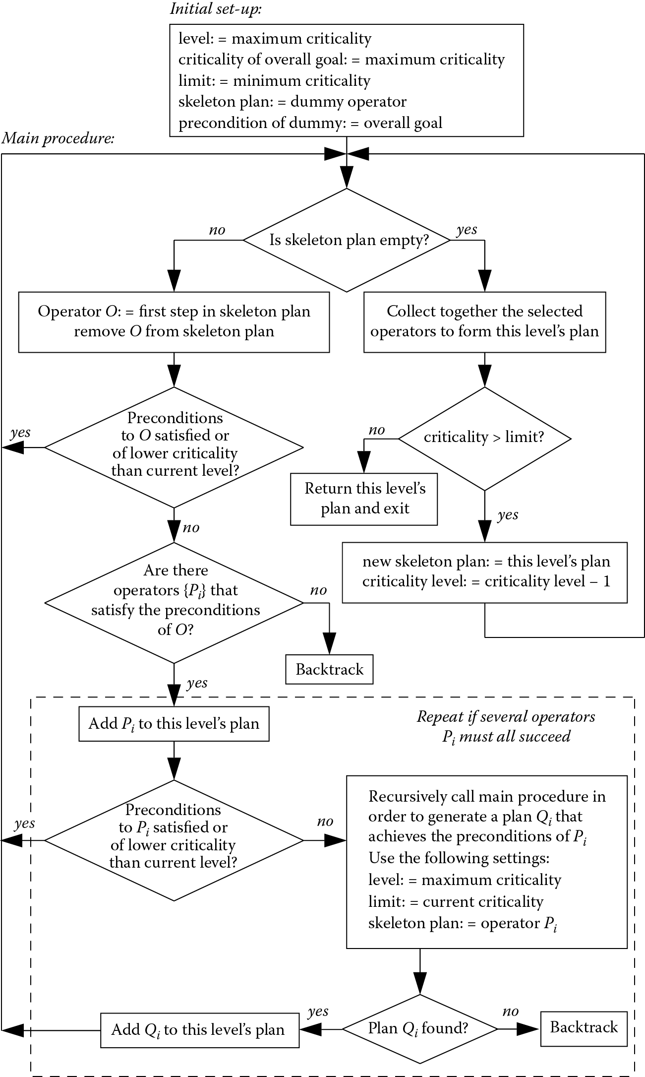
When we begin planning, a dummy operator is used to represent the skeleton plan. The precondition of dummy is the goal that we are trying to achieve. Consider planning to achieve the goal customer has product, beginning at abstraction level 5 (Figure 13.7). The precondition to dummy is customer has product. This precondition is satisfied by the operator deliver, which has two preconditions. One of them (order placed) is satisfied, and the other (product ready) has a criticality less than 5. Therefore deliver becomes the skeleton plan for a lower abstraction level.

The skeleton plan cannot be elaborated in levels 4, 3, or 2, as the criticality of product ready is only 1. At level 1, operators that achieve product ready are sought and two are found, namely, manufacture and subcontract. Both of these operators have preconditions of the highest criticality, so there is no reason to give one priority over the other. Supposing that manufacture is selected, the main procedure is then called recursively, with the preconditions to manufacture as the new goal. The precondition of the highest criticality is staff available, and this is found to be satisfied. At the next level machinery working is examined, and the main procedure is called recursively to find a plan to satisfy this precondition. However, no such plan can be found as parts available is false. The plan to manufacture is abandoned at this stage and the planner backtracks to its alternative plan, subcontract. The preconditions to subcontract are satisfied, and this becomes the plan.

A hierarchical planner can solve problems with less searching and backtracking than its nonhierarchical equivalent. The preceding example (shown in Figure 13.7) is more efficient than the STRIPS version (Figure 13.5), as the hierarchical planner did not consider the details of borrowing money and buying raw materials before abandoning the plan to manufacture. Because a complete plan is formulated at each level of abstraction before the next level is considered, the hierarchical planner can recognize dead ends early, as it did with the problem of fixing the machinery. If more complex plans are considered, involving many more operators, the saving becomes much greater still.

The planner described here, based on ABSTRIPS, is just one of many approaches to hierarchical planning. Others adopt different means of determining the hierarchical layers, since the assignment of criticalities in ABSTRIPS is rather ad hoc. Some of the other systems are less rigid in their use of a skeleton plan. For example, the Nonlin system (Tate 1977) treats the abstraction levels as a guide to a skeleton solution, but is able to replan or consider alternatives at any level if a solution cannot be found or if a higher-level choice is faulty.

13.6 Postponement of Commitment

13.6.1 Partial Ordering of Plans

We have already seen that an incentive for hierarchical planning is the notion that we are better off deferring detailed decisions until after more general decisions have been made. This is a part of the principle of postponement of commitment, or the principle of least commitment. In the same context, if the order of steps in a plan makes no difference to the plan, the planner should leave open the option of doing them in any order. A plan is said to be partially ordered if it contains actions that are unordered with respect to each other, that is, actions for which the planner has not yet determined an order and which may possibly be in parallel.

If we refer back to the Prolog planner described in Section 13.3.3, we see that, given a particular world state and the goal of supplying a product to a customer, the following plan was generated:

[borrow_money, purchase_materials, fix_machine, manufacture, deliver]

This plan contains a definite order of events. As can be inferred from the search tree in Figure 13.2, some events must occur before others. For example, the product cannot be delivered until after it has been manufactured. However, the operators fix_machine and purchase_materials have been placed in an arbitrary order. These operators are intended to satisfy two subgoals (machinery working and sufficient raw materials, respectively). As both subgoals need to be achieved, they are conjunctive goals. A planning system is said to be linear if it assumes that it does not matter in which order conjunctive goals are satisfied. This is the so-called linear assumption, which is not necessarily valid, and which can be expressed as follows:

according to the linear assumption, subgoals are independent and thus can be sequentially achieved in an arbitrary order.

Nonlinear planners are those that do not rely upon this assumption. The generation of partially ordered plans is the most common form of nonlinear planning, but it is not the only form (Hendler et al. 1990). The generation of a partially ordered plan avoids commitment to a particular order of actions until information for selecting one order in preference to another has been gathered. Thus, a nonlinear planner might generate the following partially ordered plan.

$\left[\left[\begin{array}{c}borrow\_money, purchase\_materials\\ fix\_machine\end{array}\right], manufacture, deliver\right]$

If it is subsequently discovered that fixing the machine requires us to borrow money, this can be accommodated readily because we have not committed ourselves to fixing the machine before seeking a loan. Thus, a single loan can be organized for the purchase of raw materials and for fixing the machine.

The option to generate a partially ordered plan occurs every time a planner encounters a conjunctive node (i.e., and) on the search tree. Linear planners are adequate when the branches are decoupled, so that it does not matter which action is performed first. Where the ordering is important, a nonlinear planner can avoid an exponential search of all possible plan orderings. To emphasize how enormous this saving can be, just ten actions have more than three million (i.e., 10!) possible orderings.

Some nonlinear planners (e.g., HACKER (Sussman 1975) and INTERPLAN (Tate 1975)) adopt a different approach to limiting the number of orderings that need be considered. These systems start out by making the linearity assumption. When confronted with a conjunctive node in the search tree, they select an arbitrary order for the actions corresponding to the separate branches. If the selected order is subsequently found to create problems, the plan is fixed by reordering. Depending on the problem being addressed, this approach may be inefficient as it can involve a large amount of backtracking.

HYBIS is a nonlinear planner that uses prior experience of previously solved planning problems to reduce the amount of backtracking (Fernandez et al. 2005). Goals are decomposed into subgoals at a lower level of the hierarchy, for each of which a partial order planner is evoked. The prior experience is represented as a trace of a search tree, whose nodes are tagged as previously successful, failed, abandoned, or unexplored. The previously successful nodes are prioritized for possible re-use, leading to efficiency gains.

We have already seen that the actions of one branch of the search tree can interact with the actions of another. As a further example, a system might plan to purchase sufficient raw materials for manufacturing a single batch, but some of these materials might be used up in the alignment of machinery following its repair. Detecting and correcting these interactions is a problem that has been addressed by most of the more sophisticated planners. The problem is particularly difficult in the case of planners such as SIPE that allow actions to take place concurrently. SIPE tackles the problem by allocating a share of limited resources to each action and placing restrictions on concurrent actions that use the same resources. Modeling the process in this way has the advantage that resource conflicts are easier to detect than interactions between the effects of two actions.

13.6.2 The Use of Planning Variables

The use of planning variables is another technique for postponing decisions until they have to be made. Planners with this capability could, for instance, plan to purchase something, where something is a variable that does not yet have a value assigned. Thus the planner can accumulate information before making a decision about what to purchase. The instantiation of something may be determined later, thus avoiding the need to produce and check a plan for every possible instantiation.

The use of planning variables becomes more powerful still if we can progressively limit the possible instantiations by applying constraints to the values that a variable can take. Rather than assuming that something is either unknown or has a specific value (e.g., gearbox_part#7934), we could start by applying the constraint that it is a gearbox component. We might then progressively tighten the constraints and, thereby, reduce the number of possible instantiations.

13.7 Job-Shop Scheduling

13.7.1 The Problem

As noted in Section 13.1, scheduling is a planning problem where time and resources must be allocated to operators that are known in advance. The term scheduling is sometimes applied to the internal scheduling of operations within a knowledge-based system. However, in this section we will be concerned with scheduling only in an engineering context.

Job-shop scheduling is a problem of great commercial importance. A job shop is either a factory or a manufacturing unit within a factory. Typically, the job shop consists of a number of machine tools connected by an automated palletized transportation system, as shown in Figure 13.8. The completion of a job may require the production of many different parts, grouped in lots. Flexible manufacturing is possible, because different machines can work on different part types simultaneously, allowing the job shop to adapt rapidly to changes in production mix and volume.

The planning task is to determine a schedule for the manufacturing of the parts that make up a job. As noted in Section 13.1, the operations are already known in this type of problem, but they still need to be organized in the most efficient way. The output that is required from a scheduling system is typically a Gantt chart like that shown in Figure 13.9. The decisions required are, therefore,

• the allocation of machines (or other resources) to each operation;
• the start and finish times of each operation (although it may be sufficient to specify only the order of operations, rather than their projected timings).

The output of the job shop should display graceful degradation, that is, a reduced output should be maintained in the event of accidental or preprogrammed machine stops, rather than the whole job shop grinding to a halt. The schedule must ensure that all jobs are completed before their due dates, while taking account of related considerations such as minimizing machine idle times, queues at machines, work in progress, and allowing a safety margin in case of unexpected machine breakdown. Some of these considerations are constraints that must be satisfied, and others are preferences that we would like to satisfy to some degree. Several researchers, for example, (Bruno et al. 1986) and (Dattero et al. 1989), have pointed out that a satisfactory schedule is required, and that this may not necessarily be an optimum. A similar viewpoint is frequently adopted in the area of engineering design (Chapter 12).

13.7.2 Some Approaches to Scheduling

The approaches to automated scheduling that have been applied in the past can be categorized as either analytical, iterative, or heuristic (Liu 1988). None of these approaches has been particularly successful in its own right, but some of the more successful scheduling systems borrow techniques from all three approaches. The analytical approach requires the problem to be structured into a formal mathematical model. Achieving this normally requires several assumptions to be made, which can compromise the validity of the model in real-life situations. The iterative approach requires all possible schedules to be tested and the best one to be selected. The computational load of such an approach renders it impractical where there are large numbers of machines and lots. The heuristic approach relies on the use of rules to guide the scheduling. While this can save considerable computation, the rules are often specific to just one situation, and their expressive power may be inadequate.

Bruno et al. have adopted a semiempirical approach to the scheduling problem (Bruno et al. 1986). A discrete event simulation (similar, in principle, to the ultrasonic simulation described in Chapter 4) serves as a test bed for the effects of action sequences. If a particular sequence causes a constraint to be violated, the simulation can backtrack by one or more events and then test a new sequence. Objects are used to represent the key players in the simulation, such as lots, events, and goals. Rules are used to guide the selection of event sequences using priorities that are allocated to each lot by the simple expression:

$\text{priority}=\frac{\text{remaining machining time}}{\text{due date}-\text{release time}}$

Liu (1988) has extended the ideas of hierarchical planning (Section 13.5) to include job-shop scheduling. He has pointed out that one of the greatest problems in scheduling is the interaction between events, so that fixing one problem (e.g., bringing forward a particular machining operation) can generate new problems (e.g., another lot might require the same operation, but its schedule cannot be moved forward). Liu therefore sees the problem as one of maintaining the integrity of a global plan, and dealing with the effects of local decisions on that global plan. He solves the problem by introducing planning levels. He starts by generating a rough utilization plan—typically based upon the one resource thought to be the most critical—that acts as a guideline for a more detailed schedule. The rough plan is not expanded into a more detailed plan, but rather a detailed plan is formed from scratch, with the rough plan acting as a guide.

As scheduling is an optimization problem, it is no surprise that many researchers have applied computational intelligence approaches. In the domain of scheduling pumping operations in the water distribution industry, McCormick and Powell (2004) have used simulated annealing to produce near-optimal discrete pump schedules while Gogos et al. (2005) have used genetic algorithms to optimize their mathematical model. Other researchers in the same domain have taken a hybrid approach to scheduling (e.g., AbdelMeguid and Ulanicki 2010) have used a genetic algorithm to calculate feedback rules. In fact, their approach did not outperform a traditionally produced time schedule, but it was more robust to unexpected changes in water flows and demand.

Rather than attempt to describe all approaches to the scheduling problem, one particular approach will now be described in some detail. This approach involves constraint-based analysis (CBA) coupled with the application of preferences.

13.8 Constraint-Based Analysis

13.8.1 Constraints and Preferences

A review of constraint-based analysis for planning and scheduling is provided by Bartak, Salido, and Rossi (2010). There may be many factors to take into account when generating a schedule. As noted in Section 13.7.1, some of these are constraints that must be satisfied, and others are preferences that we would like to satisfy. Whether or not a constraint is satisfied is generally clear cut, for example, a product is either ready on time or it is not. The satisfaction of preferences is sometimes clear-cut, but often it is not. For instance, we might prefer to use a particular machine. This preference is clear-cut because it will either be met or it will not. On the other hand, a preference such as “minimize machine idle times” can be met to varying degrees.

13.8.2 Formalizing the Constraints

Four types of scheduling constraints that apply to a flexible manufacturing system can be identified:

• Production constraints

  The specified quantity of goods must be ready before the due date, and quality standards must be maintained throughout. Each lot has an earliest start time and a latest finish time.

• Technological coherence constraints

  Work on a given lot cannot commence until it has entered the transportation system. Some operations must precede others within a given job, and sometimes a predetermined sequence of operations exists. Some stages of manufacturing may require specific machines.

• Resource constraints

  Each operation must have access to sufficient resources. The only resource that we will consider in this study is time at a machine, where the number of available machines is limited. Each machine can work on only one lot at a given time, and programmed maintenance periods for machines must be taken into account.

• Capacity constraints

  In order to avoid unacceptable congestion in the transportation system, machine use and queue lengths must not exceed predefined limits.

Our discussion of constraint-based analysis will be based upon Bel et al. (1989). Their knowledge-based system, OPAL, solves the static (i.e., “snapshot”) job-shop scheduling problem. It is, therefore, a classical planner (see Section 13.2). OPAL contains five modules (Figure 13.10):

• an object-oriented database for representing entities in the system such as lots, operations, and resources (including machines);
• a constraint-based analysis (CBA) module that calculates the effects of time constraints on the sequence of operations (the module generates a set of precedence relations between operations, thereby partially or fully defining those sequences that are viable);
• a decision-support module that contains rules for choosing a schedule, based upon practical or heuristic experience, from among those that the CBA module has found to be viable;
• a supervisor that controls communication between the CBA and decision-support modules, and builds up the schedule for presentation to the user;
• a user interface module.

Job-shop scheduling can be viewed in terms of juggling operations and resources. Operations are the tasks that need to be performed in order to complete a job, and several jobs may need to be scheduled together. Operations are characterized by their start time and duration. Each operation normally uses resources, such as a length of time at a given machine. There are two types of decisions, the timing or (sequencing) of operations and the allocation of resources. For the moment we will concentrate on the CBA module, which is based upon the following set of assumptions:

• There is a set of jobs J comprised of a set of operations O.
• There is a limited set of resources R.
• Each operation has the following properties:
  • cannot be interrupted;
  • uses a subset r of the available resources;
  • uses a quantity qi of each resource ri in the set r;
  • has a fixed duration di.

A schedule is characterized by a set of operations, their start times, and their durations. We will assume that the operations that make up a job and their durations are predefined. Therefore, a schedule can be specified by just a set of start times for the operations. For a given job, there is an earliest start time (esti) and latest finish time (lfti) for each operation Oi. Each operation has a time window which it could occupy and a duration within that window that it will occupy. The problem is then one of positioning the operation within the window as shown in Figure 13.11.

13.8.3 Identifying the Critical Sets of Operations

The first step in the application of CBA is to determine if and where conflicts for resources arise. These conflicts are identified through the use of critical sets, a concept that is best described by example. Suppose that a small factory employs five workers who are suitably skilled for carrying out a set of four operations Oi. Each operation requires some number qi of the workers, as shown in Table 13.4.

A critical set of operations Ic is one that requires more resources than are available, but where this conflict would be resolved if any of the operations were removed from the set. In our example, the workers are the resource and the critical sets are {O1,O3}, {O2,O3}, {O4,O3}, {O1,O2,O4}. Note that {O1,O2,O3} is not a critical set since it would still require more resources than the five available workers if we removed O1 or O2. The critical sets define the conflicts for resources, because the operations that make up the critical sets cannot be carried out simultaneously. Therefore, the first sequencing rule is as follows:

one operation of each critical set must precede at least one other operation in the same critical set.

Applying this rule to the preceding example produces the following conditions:

These conditions have been deduced purely on the basis of the available resources, without consideration of time constraints. If we now introduce the known time constraints (i.e., the earliest start times and latest finish times for each operation), the schedule of operations can be refined further and, in some cases, defined completely. The schedule of operations is especially constrained in the case where each conflict set is a pair of operations. This is the disjunctive case, which we will consider first before moving on to consider the more general case.

13.8.4 Sequencing in Disjunctive Case

As each conflict set is a pair of operations in the disjunctive case, no operations can be carried out simultaneously. Each operation has a defined duration (di), an earliest start time (esti), and a latest finish time (lfti). The scheduling task is one of determining the actual start time for each operation.

Consider the task of scheduling the three operations A, B, and C shown in Figure 13.12. If we try to schedule operation A first, we find that there is insufficient time for the remaining operations to be carried out before the last lft, irrespective of how the other operations are ordered (Figure 13.12). However, there is a feasible schedule if operation C precedes A. This observation is an example of the following general rule, informally stated:

rule r13_1 /* informally stated; not Flex format */

	if (latest lft - estA) < Σdi

	then at least one operation must precede A.

Similarly, there is no feasible schedule that has A as the last operation since there is insufficient time to perform all operations between the earliest est and the lft for A (Figure 13.12). The general rule that describes this situation is:

rule r13_2 /* informally stated; not Flex format */

	if (lftA - earliest est) < Σdi

	then at least one operation must follow A.

13.8.5 Sequencing in Nondisjunctive Case

In the nondisjunctive case, at least one critical set contains more than two operations. The precedence rules described earlier can be applied to those critical sets that contain only two operations. Let us consider the precedence constraints that apply to the operations Oi of a critical set having more than two elements. From our original definition of a critical set, it is not possible for all of the operations in the set to be carried out simultaneously. At any one time, at least one operation in the set must either have finished or be waiting to start. This provides the basis for some precedence relations. Let us denote the critical set by the symbol S, where S includes the operation A. Another set of operations that contains all elements of S apart from operation A will be denoted by the letter W. The two precedence rules that apply are as follows:

rule r13_3 /* informally stated; not Flex format */

	if (lfti-estj) < (di + dj) for every pair of operations {Oi, Oj} in set W

	/* condition that Oi cannot be performed after Oj has finished */

	and lfti-estA < dA + di for every operation Oi in set W

	/* condition that Oi cannot be performed after A has finished) */

	then at least one operation in set W must have finished before A starts.

rule r13_4 /* informally stated; not Flex format */

	if (lfti-estj) < (di + dj) for every pair of operations {Oi, Oj} in set W

	/* condition that Oi cannot be performed after Oj has finished */

	and (lftA-esti) < (dA + di) for every operation Oi in set W

	/* condition that A cannot be performed after Oi has finished) */

	then A must finish before at least one operation in set W starts.

The application of rule r13_3 is shown in Figure 13.13. Operations B and C have to overlap (the first condition) and it is not possible for A to finish before one of either B or C has started (the second condition). Therefore, operation A must be preceded by at least one of the other operations. Note that, if this is not possible either, there is no feasible schedule. (Overlap of all the operations is unavoidable in such a case, but since we are dealing with a critical set there is insufficient resource to support this.)

Rule r13_4 is similar and covers the situation depicted in Figure 13.13. Here operations B and C again have to overlap, and it is not possible to delay the start of A until after one of the other operations has finished. Under these circumstances operation A must precede at least one of the other operations.

13.8.6 Updating Earliest Start Times and Latest Finish Times

If rule r13_1 or r13_3 has been fired, so we know that at least one operation must precede A, it may be possible to update the earliest start time of A to reflect this restriction, as shown in Figure 13.14 and Figure 13.14. The rule that describes this is:

rule r13_5 /* informally stated; not Flex format */

	if some operations must precede A /* by rule r13_1 or r13_3 */

	and [the earliest (est+d) of those operations] > estA

	then the new estA is the earliest (est+d) of those operations.

Similarly, if rule r13_2 or r13_4 has been fired, so we know that at least one operation must follow operation A, it may be possible to modify the lft for A, as shown in Figure 13.14 and Figure 13.14. The rule that describes this is:

rule r13_6 /* informally stated; not Flex format */

	if some operations must follow A /* by rule r13_2 or r13_4 */

	and [the latest (lft-d) of those operations] < lftA

	then the new lftA is the latest (lft-d) of those operations.

The new earliest start times and latest finish times can have an effect on subsequent operations. Consider the case of a factory that is assembling cars. Axle assembly must precede wheel fitting, regardless of any resource considerations. This sort of precedence relation, which is imposed by the nature of the task itself, is referred to as a technological coherence constraint. Suppose that, as a result of the arguments described earlier, the est for axle assembly is delayed to a new time esta. If the axle assembly takes time da per car, then the new est for wheel-fitting (estw) will be esta+da (ignoring the time taken to move the vehicle between assembly stations).

However, a car plant is unlikely to be moving just one car through the assembly process, rather a whole batch of cars will need to be scheduled. These circumstances offer greater flexibility as the two assembly operations can overlap, provided that the order of assembly is maintained for individual cars. Two rules can be derived, depending on whether axle assembly or wheel fitting is the quicker operation. If wheel fitting is quicker, then a sufficient condition is for wheels to be fitted to the last car in the batch immediately after its axles have been assembled. This situation is shown in Figure 13.15, and is described by the following rule:

rule r13_7 /* informally stated; not Flex format */

	if da > dw

	then estw becomes esta + Da - (n-1)dw

	and lfta becomes lftw – dw.

where n is the number of cars in the batch, Da is nda, and Dw is ndw. If axle assembly is the quicker operation, then wheel fitting can commence immediately after the first car has had its axle assembled (Figure 13.15). The following rule applies:

rule r13_8 /* informally stated; not Flex format */

	if da < dw

	then estw becomes esta + da

	and lfta becomes lftw - Dw + (n-1)da.

13.8.7 Applying Preferences

Constraint-based analysis can produce one of three possible outcomes:

• The constraints cannot be satisfied, given the allocated resources.
• A unique schedule is produced that satisfies the constraints.
• More than one schedule is found that satisfies the constraints.

In the case of the first outcome, the problem can be solved only if more resources are made available or the time constraints are slackened. In the second case, the scheduling problem is solved. In the third case, pairs of operations exist that can be sequenced in either order without violating the constraints. The problem then becomes one of applying preferences so as to find the most suitable order. Preferences are features of the solution that are considered desirable but, unlike constraints, they are not compulsory. Preferences can be applied by using fuzzy rules (Bel et al. 1989). Such a fuzzy rule-based system constitutes the decision-support module in Figure 13.10. (See Chapter 3, Sections 3.4–3.6 for a discussion of fuzzy logic.)

The pairs of operations that need to be ordered are potentially large in number and broad in scope. It is, therefore, impractical to produce a rule base that covers specific pairs of operations. Instead, rules for applying preferences usually make use of local variables (see Chapter 2, Section 2.6), so that they can be applied to different pairs of operations. The rules may take the form:

rule r13_9 /* informally stated; not Flex format */

	if (x of Operation1) > (x of Operation2)

	then Operation1 precedes Operation2.

where any pair of operations can be substituted for Operation1 and Operation2, but the attribute x is specified in a given rule. A typical expression for x might be the duration of its available time window (i.e., lft–est). The rules are chosen so as to cover some general guiding principles or goals, such as:

• Maximize overall slack time.
• Perform operations with the least slack time first.
• Give preference to schedules that minimize resource utilization.
• Avoid tool changes.

In OPAL, each rule is assigned a degree of relevance R with respect to each goal. Given a goal or set of goals, some rules will tend to favor one ordering of a pair of operations, while others will favor the reverse. A consensus is arrived at by a scoring (or ‘voting’) procedure. The complete set of rules is applied to each pair of operations that need to be ordered, and the scoring procedure is as follows:

• The degree to which the condition part of each rule is satisfied is represented using fuzzy sets. Three fuzzy sets are defined (true, maybe, and false), and the degree of membership of each is designated µt, µm, and µf. Each membership is a number between 0 and 1, such that for every rule:

µt + µm + µf = 1

• Every rule awards a score to each of the three possible outcomes (a precedes b, b precedes a, or no preference). These scores (Vab, Vba, and Vno_preference) are determined as follows:

Vab = min(µt , R)

Vba = min(µf , R)

Vno_preference = min(µm, R)

• The scores for each of the three possible outcomes are totaled across the whole rule set. The totals can also be normalized by dividing the sum of the scores by the sum of the R values for all rules. Thus:

Total score for ab = Σ(Vab)/Σ(R)

Total score for ba = Σ(Vba)/Σ(R)

Total score for no preference = Σ(Vno_preference)/Σ(R)

The scoring procedure can have one of three possible outcomes:

• One ordering is favored over the other. This outcome is manifested by Σ(Vab) » Σ(Vba) or vice versa.
• Both orderings are roughly equally favored, but the scores for each are low compared with the score for the impartial outcome. This indicates that there is no strong reason for preferring one order over the other.
• Both orderings are roughly equally favored, but the scores for each are high compared with the score for the impartial outcome. Under these circumstances, there are strong reasons for preferring one order, but there are also strong reasons for preferring the reverse order. In other words there are strong conflicts between the rules.

13.8.8 Using Constraints and Preferences

OPAL makes use of a supervisor module that controls the constraint-based analysis (CBA) and decision support (DS) modules (Figure 13.10). In OPAL and other scheduling systems, constraint-based analysis is initially applied in order to eliminate all those schedules that cannot meet the time and resource constraints. A preferred ordering of operations is then selected from the schedules that are left. As we have seen, the DS module achieves this by weighting the rules of optimization, applying these rules, and selecting the order of operations that obtains the highest overall score.

If the preferences applied by the DS module are not sufficient to produce a unique schedule, the supervising module calls upon the CBA and DS modules repeatedly until a unique solution is found. The supervising module stops the process when an acceptable schedule has been found, or if it cannot find a workable schedule.

There is a clear analogy between the two stages of scheduling (constraint-based analysis and the application of preferences) and the stages of materials selection (see Chapter 12, Section 12.8). In the case of materials selection, constraints can be applied by ruling out all materials that fail to meet a numerical specification. The remaining materials can then be put into an order of preference, based upon some means of comparing their performance scores against various criteria, where the scores are weighted according to a measure of the perceived importance of the properties.

13.9 Replanning and Reactive Planning

The discussion so far has concentrated on predictive planning, that is, building a plan that is to be executed at some time in the future. Suppose now that, while a plan is being executed, something unexpected happens, such as a machine breakdown. In other words, the actual world state deviates from the expected world state. A powerful capability under these circumstances is to be able to replan, i.e., to modify the current plan to reflect the current circumstances. Systems that are capable of planning or replanning in real time, in a rapidly changing environment, are described as reactive planners. Such systems monitor the state of the world during execution of a plan and are capable of revising the plan in response to their observations. Since a reactive planner can alter the actions of machinery in response to real-time observations and measurements, the distinction between reactive planners and control systems (Chapter 14) is blurred.

To illustrate the distinction between predictive planning, replanning, and reactive planning, let us consider an intelligent robot that is carrying out some gardening. It may have planned in advance to mow the lawn and then to prune the roses (predictive planning). If it finds that someone has borrowed the mower, it might decide to mow after pruning, by which time the mower may have become available (replanning). If a missile is thrown at the robot while it is pruning, it may choose to dive for cover (reactive planning).

Collinot et al. have devised a system called SONIA (Collinot et al. 1988), that is capable of both predictive and reactive planning of factory activity. This system offers more than just a scheduling capability, as it has some facilities for selecting which operations will be scheduled. However, it assumes that a core of essential operations is preselected. SONIA brings together many of the techniques that we have seen previously. The operations are ordered by the application of constraints and preferences (Section 13.8) in order to form a predictive plan. During execution of the plan, the observed world state may deviate from the planned world state. Some possible causes of the deviation might be:

• machine failure;
• personnel absence;
• arrival of urgent new orders;
• the original plan may have been ill-conceived.

Under these circumstances, SONIA can modify its plan or, in an extreme case, generate a new plan from scratch. The particular type of modification chosen is largely dependent on the time available for SONIA to reason about the problem. Some possible plan modifications might be:

• cancel, postpone, or curtail some operations in order to bring some other operations back on schedule;
• reschedule to use any slack time in the original plan;
• reallocate resources between operations;
• reschedule a job—comprising a series of operations—to finish later than previously planned;
• delay the whole schedule.

A final point to note about SONIA is that it has been implemented as a blackboard system (see Chapter 9). The versatility of the blackboard architecture is demonstrated by the variety of applications in which it is used. An application in data interpretation was described in Chapter 11, whereas here it is used for predictive planning. SONIA uses the blackboard to represent both the planned and observed world states. Separate agents perform the various stages of predictive planning, monitoring, and reactive planning. In fact, SONIA uses two blackboards: one for representing information about the shop floor and a separate one for its own internal control information.

13.10 Summary

This chapter began by defining a classical planner as one that can derive a set of operations to take the world from an initial state to a goal state. The initial world state is a “snapshot” that is assumed not to alter except as a result of the execution of the plan. While being useful in a wide range of situations, classical planners are of limited use when dealing with continuous processes or a rapidly changing environment. In contrast, reactive planners can respond rapidly to unexpected events.

Scheduling is a special case of planning, where the operators are known in advance and the task is to allocate resources to each and to determine when they should be applied. Scheduling is particularly important in the planning of manufacturing processes.

A simple classical planner similar to STRIPS has been described. More sophisticated features that can be added to extend the capabilities of a planning system were then described and are summarized as follows:

• World modeling

  Unlike STRIPS, the Prolog program shown in Section 13.3.3 does not explicitly update its world model as operators are selected. Proper maintenance of a world model ensures that any side effects of a plan are recorded along with intended effects.

• Deductive rules

  Deductive rules permit the deduction of effects that are additional to those explicitly included in the operator representation. Because they do not form part of the operator representation, they can allow different effects to be registered depending on the current context.

• Hierarchical planning

  STRIPS may commit itself to a particular problem-solving path too early, with the result that it must backtrack if it cannot complete the plan that it is pursuing. Hierarchical planners can plan at different levels of abstraction. An abstract (or “skeleton”) plan is formed first, such as to build a house by digging foundations, then building walls, and finally putting on a roof. The detailed planning might include the precise shape, size, and placement of the timber. The abstract plan restricts the range of possibilities of the detailed planning.

• Nonlinearity

  Linear planners such as STRIPS make the assumption that it does not matter in which order the subgoals for a particular goal are satisfied. Partial ordering of operations is a form of nonlinear planning in which the ordering of operations is postponed until either more information becomes available or a decision is forced. In some cases, it may be possible for operations to be scheduled to run in parallel.

• Planning variables

  The use of variables also allows postponement of decisions. Plans can be generated using variables that have not yet been assigned a value. For instance, we might plan to go somewhere without specifying where. The instantiation of somewhere may become determined later, and we have saved the effort of considering all of the possibilities in the meantime.

• Constraints

  The use of planning variables is more powerful still if we can limit the possible instantiations by applying constraints on the values that a variable can take. Constraint-based analysis can be used to reduce the number of possible plans, or even to find a unique plan that meets the constraints.

• Preferences

  If constraint-based analysis yields more than one viable plan or schedule, preferences can be applied in order to select between the alternatives.

• Replanning

  The ability to modify a plan in the light of unexpected occurrences was discussed.

Hierarchical plans, partially ordered plans, and the use of planning variables are all means of postponing commitment to a particular plan. This is known as the principle of least commitment.

Systems that have only some of the aforementioned features are adequate in many situations. A few specific applications have been considered in this chapter, but much of the research effort in planning has been concerned with building general purpose planning systems that are domain-independent. The purpose of such systems is to allow knowledge relevant to any particular domain to be represented, rather like an expert system shell (see Chapters 1 and 10).

Further Reading

van Wezel, W., R. J. Jorna, and A. M. Meystel. 2006. Planning in Intelligent Systems: Aspects, Motivations, and Methods. Wiley.

Vlahavas, I., and D. Vrakas. 2004. Intelligent Techniques for Planning. IGI Publishing, Hershey, PA.

Wilkins, D. E. 1989. Practical Planning: Extending the Classical AI Planning Paradigm. Edited by R. J. Brachman. Morgan Kaufmann, San Francisco, CA.

Yang, Q. 1998. Intelligent Planning: A Decomposition and Abstraction-Based Approach. Springer Verlag, Berlin.