Chapter 9

Hybrid Systems

9.1 Convergence of Techniques

The previous chapters of this book have demonstrated that there is a wide variety of computing techniques that can be applied to particular problems. These include knowledge-based systems, computational intelligence methods, and conventional programs. In many cases the techniques need not be exclusive alternatives to each other but can be seen as complementary tools that can be brought together within a hybrid system. All of the techniques reviewed in this book can, in principle, be mixed with other techniques. This chapter is structured around four ways in which different computational techniques can be complementary:

• Dealing with multifaceted problems. Most real-life problems are complex and have many facets, where each facet may be best suited to a different technique. Therefore, many practical systems are designed as hybrids, incorporating several specialized modules, each of which uses the most suitable tools for its specific task. One way of allowing the modules to communicate is by designing the hybrid as a blackboard system, described in Section 9.2.
• Parameter setting. Several of the techniques described in this chapter, such as genetic-fuzzy and genetic-neural systems, are based on the idea of using one technique to set the parameters of another.
• Capability enhancement. One technique may be used within another to enhance the latter’s capabilities. For example, Lamarckian or Baldwinian inheritance involves the inclusion of a local-search step within a genetic algorithm. In this case, the aim is to raise the fitness of individual chromosomes and to speed convergence of the genetic algorithm toward an optimum.
• Clarification and verification. Neural networks have the ability to learn associations between input vectors and associated outputs. However, the underlying reasons for the associations are opaque, as they are effectively encoded in the weightings on the interconnections between the neurons. Efforts have been made to extract equivalent rules from the network automatically. The extracted rules can be more readily understood than the interconnection weights from which they are derived. Verification rules can apply additional knowledge to check the validity of the network’s output.

9.2 Blackboard Systems for Multifaceted Problems

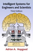
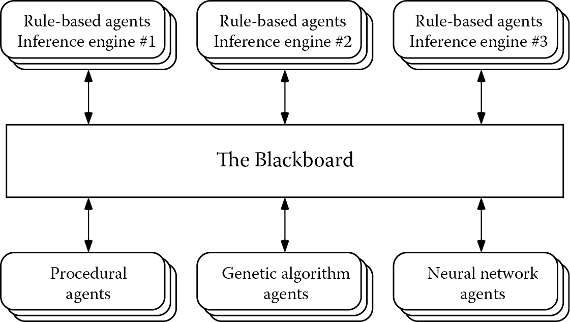
The blackboard model or blackboard architecture, shown in Figure 9.1, provides a software structure that is well suited to multifaceted tasks. Systems that have this kind of structure are called blackboard systems. In a blackboard system, knowledge of the application domain is divided into modules. These modules were historically referred to as knowledge sources (or KSs) but, as they are independent and autonomous, they are now commonly regarded as agents. Each agent is designed to tackle a particular subtask. The agents are independent and can communicate only by reading from or writing to the blackboard, a globally accessible working memory where the current state of understanding is represented. The agents can also delete unwanted information from the blackboard.

The first published application of a blackboard system was Hearsay-II for speech understanding in 1975 (Erman et al. 1980; Lesser et al. 1975). Further developments took place during the 1980s (Nii 1986). In the late 1980s, the Algorithmic and Rule-Based Blackboard System (ARBS) was developed and subsequently applied to diverse problems including the interpretation of ultrasonic images (Hopgood et al. 1993), the management of telecommunications networks (Hopgood 1994), and the control of plasma deposition processes (Hopgood et al. 1998). Later, ARBS was redesigned as a distributed system, DARBS, in which the software modules run in parallel, possibly on separate computers connected via the Internet (Nolle et al. 2001; Tait et al. 2008). DARBS is now freely available as open-source software.* The blackboard model is now widely seen as a key technology for multiagent systems (Brzykcy et al. 2001).

A blackboard system is analogous to a team of experts who communicate their ideas via a physical blackboard, by adding or deleting items in response to the information that they find there. Each agent represents such an expert having a specialized area of knowledge. As each agent can be encoded in the most suitable form for its particular task, blackboard systems offer a mechanism for the collaborative use of different computational techniques such as rules, neural networks, genetic algorithms, and fuzzy logic. The inherent modularity of a blackboard system is also helpful for maintenance. Each rule-based agent can use a suitable reasoning strategy for its particular task, for example, forward chaining or backward chaining, and can be thought of as a rule-based system in microcosm.

Agents are applied in response to information on the blackboard, when they have some contribution to make. This leads to increased efficiency, since the detailed knowledge within an agent is only applied when that agent becomes relevant. The agents are said to be opportunistic, activating themselves whenever they can contribute to the global solution. In early, nondistributed backboard systems, true opportunism was difficult to achieve as it required explicit scheduling and could involve interrupting an agent that was currently active. In modern blackboard systems, each agent is its own process, either in parallel with other agents on multiple processors or concurrently on a single processor, so no explicit scheduling is required.

In the interests of efficiency and clarity, some degree of structure is usually imposed on the blackboard by dividing it into partitions. An agent then only needs to look at a partition rather than the whole blackboard. Typically, the blackboard partitions correspond to different levels of analysis of the problem, progressing from detailed information to more abstract concepts. In the Hearsay-II blackboard system for computerized understanding of natural speech, the levels of analysis include those of syllable, word, and phrase (Erman et al. 1980). In ultrasonic image interpretation using ARBS, described in more detail in Chapter 11, the levels progress from raw signal data, via a description of the significant image features, to a description of the defects in the component (Hopgood et al. 1993).

The key advantages of the blackboard architecture can be summarized as follows (Feigenbaum 1988):

• Many and varied sources of knowledge can participate in the development of a solution to a problem.
• Since each agent has access to the blackboard, each can be applied as soon as it becomes appropriate. This is opportunism, that is, application of the right knowledge at the right time.
• For many types of problems, especially those involving large amounts of numerical processing, the characteristic style of incremental solution development is particularly efficient.
• Different types of reasoning strategy (for example, data-driven and goal-driven) can be mixed as appropriate in order to reach a solution.
• Hypotheses can be posted onto the blackboard for testing by other agents. A complete test solution does not have to be built before deciding to modify or abandon the underlying hypothesis.
• In the event that the system is unable to arrive at a complete solution to a problem, the partial solutions appearing on the blackboard are available and may be of some value.

9.3 Parameter Setting

Designing a suitable solution for a given application can involve a large amount of trial and error. Although computational intelligence methods avoid the “knowledge acquisition bottleneck” that was mentioned in Chapter 5, Section 5.4 in relation to knowledge-based systems, a “parameter-setting bottleneck” may be introduced instead. The techniques described here are intended to avoid this bottleneck by using one computational intelligence technique to set the parameters of another.

9.3.1 Genetic–Neural Systems

Part of the practical challenge in building a practical neural network is to choose the right architecture and the right learning parameters. Neural networks can suffer from a parameter-setting bottleneck as the developer struggles to configure a network for a particular problem (Woodcock et al. 1991). Whether a network will converge, that is, learn suitable weightings, will depend on the topology, the transfer function of the nodes, the values of the parameters in the training algorithm, and the training data. The ability to converge may even depend on the order in which the training data are presented.

Although Kolmogorov’s Existence Theorem (see Chapter 8) leads to the conclusion that a three-layered perceptron, with the sigmoid transfer function, can perform any mapping from a set of inputs to the desired outputs, the theorem tells us nothing about the learning parameters, the necessary number of neurons, or whether additional layers would be beneficial. It is, however, possible to use a genetic algorithm to optimize the network configuration (Yao 1999). A suitable cost function might combine the RMS error with duration of training.

Supervised training of a neural network involves adjusting its weights until the output patterns obtained for a range of input patterns are as close as possible to the desired patterns. The different network topologies use different training algorithms for achieving this weight adjustment, typically through back-propagation or errors. Just as it is possible for a genetic algorithm to configure a network, it is also possible to use a genetic algorithm to train the network (Yao 1999). This can be achieved by letting each gene represent a network weight, so that a complete set of network weights is mapped onto an individual chromosome. Each chromosome can be evaluated by testing a neural network with the corresponding weights against a series of test patterns. A fitness value can be assigned according to the error, so that the weights represented by the fittest generated individual correspond to a trained neural network.

9.3.2 Genetic–Fuzzy Systems

The performance of a fuzzy system depends on the definitions of the fuzzy sets and on the fuzzy rules. As these parameters can all be expressed numerically, it is possible to devise a system whereby they are learned automatically using genetic algorithms. A chromosome can be devised that represents the complete set of parameters for a given fuzzy system. The cost function could then be defined as the total error when the fuzzy system is presented with a number of different inputs with known desired outputs.

Often, a set of fuzzy rules for a given problem can be drawn up fairly easily, but defining the most suitable membership functions remains a difficult task. Karr (Karr 1991a, 1991b) has performed a series of experiments to demonstrate the viability of using genetic algorithms to specify the membership functions. In Karr’s scheme, all membership functions are triangular. The variables are constrained to lie within a fixed range, so the fuzzy sets low and high are both right-angle triangles (Figure 9.2). The slope of these triangles can be altered by moving their intercepts on the abscissa, marked max1 and min4 in Figure 9.2. All intermediate fuzzy sets are assumed to have membership functions that are isosceles triangles. Each is defined by two points, maxi and mini, where i labels the fuzzy set. The chromosome is then a list of all the points maxi and mini that determine the complete set of membership functions. In several demonstrator systems, Karr’s GA-modified fuzzy controller outperformed a fuzzy controller whose membership functions had been set manually. This success demonstrates that tuning the fuzzy sets is a numerical optimization problem.

9.4 Capability Enhancement

One technique may be used within another to enhance the latter’s capabilities. Here, three examples are described: neuro–fuzzy systems, which combine the benefits of neural networks and fuzzy logic; Lamarckian and Baldwinian inheritance for enhancing the performance of a genetic algorithm with local search around individuals in the population; and learning classifier systems that use genetic algorithms to discover rules.

9.4.1 Neuro–Fuzzy Systems

Section 9.3.2 showed how a genetic algorithm can be used to optimize the parameters of a fuzzy system. In such a scheme, the genetic algorithm for parameter setting and the fuzzy system that uses those parameters are distinct and separate. The parameters for a fuzzy system can also be learned using neural networks, but here much closer integration is possible between the neural network and the fuzzy system that it represents. A neuro–fuzzy system is a fuzzy system, the parameters of which are derived by a neural network learning technique. It can equally be viewed as a neural network that represents a fuzzy system. The two views are equivalent and it is possible to express a neuro–fuzzy system in either form.

Consider the following fuzzy rules, based on the example used in Chapter 3:

fuzzy_rule r9_1f

	if temperature is high

	or water_level is high

	then pressure becomes high.

fuzzy_rule r9_2f

	if temperature is medium

	or water_level is medium

	then pressure becomes medium.

fuzzy_rule r9_3f

	if temperature is low

	or water_level is low

	then pressure becomes low.

These fuzzy rules and the corresponding membership functions can be represented by the neural network shown in Figure 9.3. The first stage is fuzzification, in which any given input value for temperature is given a membership value for low, medium, and high. A single-layer perceptron, designated level 1 in Figure 9.3, can achieve this because it is a linear classification task. The only difference from other classifications met previously is that the target output values are not just 0 and 1, but any value in the range 0–1. A similar network is required at level 1 for the other input variable, water_level. The neurons whose outputs correspond to the low, medium, and high memberships are marked L, M, and H, respectively, in Figure 9.3.

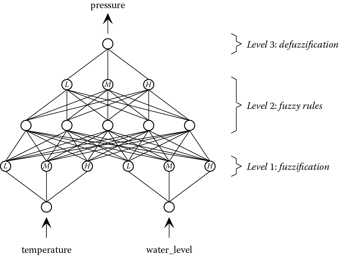
Level 2 of the neuro–fuzzy network performs the role of the fuzzy rules, taking the six membership values as its inputs and generating as its outputs the memberships for low, medium, and high of the fuzzy variable pressure. The final stage, at level 3, involves combining these membership values to produce a defuzzified value for the output variable.

The definitions of the fuzzy sets and the fuzzy rules are implicit in the connections and weights of the neuro–fuzzy network. Using a suitable learning mechanism, the weights can be learned from a series of examples. The network can then be used on previously unseen inputs to generate defuzzified output values. In principle, the fuzzy sets and rules can be inferred from the network and run as a fuzzy rule-based system, of the type described in Chapter 3, to produce identical results (Altug et al. 1999; Chow et al. 1999).

The popular ANFIS (adaptive-network-based fuzzy inference system) is based on similar principles. It uses a multilayered feedforward neural network known as an adaptive network, in which each node performs a specific function dependent on its input data and individual parameters (Jang 1993).

9.4.2 Baldwinian and Lamarckian Inheritance in Genetic Algorithms

Capability enhancement of a genetic algorithm can be achieved by hybridizing it with local search procedures. This form of hybridization can help the genetic algorithm to optimize individuals within the population, while maintaining the GA’s ability to explore the search space. The aim would be either to increase the quality of the solutions, so they are closer to the global optimum, or to increase the efficiency, that is, the speed at which the optimum is found. One approach is to introduce an extra step involving local search in the immediate vicinity of each chromosome in the population, to see whether any of its neighbors offers a fitter solution.

A commonly used, if rather artificial, example is to suppose that the task is to find the maximum denary integer represented by a seven-bit binary-encoded chromosome. The optimum is clearly 1111111. A chromosome’s fitness could be taken as the highest integer represented either by itself or by any of its near neighbors found by local search. A near neighbor of an individual might typically be defined as one that has a Hamming separation of 1 from it, that is, one bit is different. For example, the chromosome 0101100 (denary value 44) would have a fitness of 108, since it has a nearest neighbor 1101100 (denary value 108). The chromosome could be either:

1. replaced by the higher scoring neighbor, in this case 1101100 (this is Lamarckian inheritance) or
2. left unchanged while retaining the fitness value of its fittest neighbor (this is Baldwinian inheritance).

The first scheme, in which the chromosome is replaced by its fitter neighbor, is named after Lamarck (Lamarck 1809). Lamarck believed that, in nature, offspring can genetically inherit their parents’ learned characteristics and behaviors. Although this concept is a controversial view of nature, it is nevertheless a useful technique for genetic algorithms, which are inspired by nature but do not need to be an accurate biological simulation.

In the alternative scheme, Baldwinian inheritance, the chromosome is unchanged but a higher fitness is ascribed to it to acknowledge its proximity to a fitter solution. This model is named after Baldwin’s view of biological inheritance (Baldwin 1896), which is now widely accepted in preference to Lamarck’s. Baldwin argued that, although learned characteristics and behaviors cannot be inherited genetically, the capacity to learn such characteristics and behaviors can be.

Elmihoub et al. (2004, 2006b) have set out to establish the relative benefits of the two forms of inheritance. In a series of experiments, they have adjusted the relative proportions of Lamarckian and Baldwinian inheritance, and the probability of applying a local steepest-gradient descent search to any individual in the population. Their results for a four-dimensional Shwefel function (Schwefel 1981) are shown in Figure 9.4. They have shown that the optimal balance between the two forms of inheritance depends on the population size, the probability of local search and the nature of the fitness landscape (Elmihoub et al. 2006a; Hopgood 2005). With this in mind, they have also experimented with making these parameters self-adaptive by coding them within the chromosomes. Taking this idea to its logical conclusion, a completely self-adapting genetic algorithm could be envisaged where no parameters at all need to be specified by the user.

9.4.3 Learning Classifier Systems

Holland’s learning classifier systems (LCSs) combine genetic algorithms with rule-based systems to provide a mechanism for rule discovery (Holland and Reitman 1978; Goldberg 1989). The rules are simple production rules (see Chapter 2, Section 2.1), coded as a fixed-length mixture of binary numbers and wild-card, that is, “don’t care” characters. Their simple structure makes it possible to generate new rules by means of a genetic algorithm.

The overall LCS is illustrated in Figure 9.5. At the heart of the system is the message list, which fulfills a similar role to the blackboard in a blackboard system. Information from the environment is placed here, along with rule deductions and instructions for the actuators that act on the environment.

A credit-apportionment system, known as the bucket-brigade algorithm, is used to maintain a credit balance for each rule. The genetic algorithm uses a rule’s credit balance as the measure of its fitness. Conflict resolution (see Chapter 2, Section 2.8) between rules in the conflict set is achieved via an auction, in which the rule with the most credits is chosen to fire. In doing so, it must pay some of its credits to the rules that led to its conditions being satisfied. If the fired rule leads to some benefit in the environment, it receives additional credits.

9.5 Clarification and Verification of Neural Network Outputs

Neural networks have the ability to learn associations between input vectors and their associated outputs. However, the underlying reasons for the associations may be opaque, as the associations are effectively encoded in the weightings on the interconnections between the neurons. A neural network is therefore often described as a “black box,” with an internal state that conveys no readily useful information to an observer. This metaphor implies that the inputs and outputs have significance for an observer, but the weights on the interconnections between the neurons do not. This analogy contrasts with a transparent system, such as a KBS, where the internal state, that is, the value of a variable, does have meaning for an observer.

There has been considerable research into rule extraction. Here, the aim is to produce automatically a set of intelligible rules that are equivalent to the trained neural network from which they have been extracted (Tsukimoto 2000). A variety of methods have been reported for extracting different types of rules, including production rules and fuzzy rules.

In safety-critical systems, reliance on the output from a neural network without any means of verification is not acceptable. It has, therefore, been proposed that rules be used to verify that the neural network output is consistent with its input (Picton et al. 1991). The use of rules for verification implies that at least some of the domain knowledge can be expressed in rule form.

Johnson et al. (Johnson et al. 1990) suggest that an adjudicator module be used to decide whether a set of rules or a neural network is likely to provide the more reliable output for a given input. The adjudicator would have access to information relating to the extent of the neural network’s training data and could determine whether a neural network would have to interpolate between, or extrapolate from, examples in the training set. This is important, since neural networks are good at interpolation but poor at extrapolation. The adjudicator may, for example, call upon rules to handle the exceptional cases that would otherwise require a neural network to extrapolate from its training data. If heuristic rules are also available for the less exceptional cases, then they could be used to provide an explanation for the neural network’s findings. A supervisory rule-based module could dictate the training of a neural network, deciding how many nodes are required, adjusting the learning rate as training proceeds, and deciding when training should terminate.

9.6 Summary

This section has looked at just some of the ways in which different computation techniques—including intelligent systems and conventional programs—can work together within hybrid systems. Chapters 11 through 14 deal with applications of intelligent systems in engineering and science, most of which involve hybrids of some sort.

Further Reading

Castillo, O., P. Melin, and W. Pedrycz, eds. 2010. Hybrid Intelligent Systems: Analysis and Design. Springer, Berlin.

Craig, I. 1995. Blackboard Systems. Intellect, Bristol, UK.

Jain, L. C., and N. M. Martin, eds. 1999. Fusion of Neural Networks, Fuzzy Sets, and Genetic Algorithms: Industrial Applications. CRC Press, Boca Raton, FL.

---