
Chapter 3
Handling Uncertainty: Probability and Fuzzy Logic
3.1 Sources of Uncertainty
The discussion of rule-based systems in Chapter 2 assumed that we live in a clear-cut world where every hypothesis is either true, false, or unknown. Furthermore, it was pointed out that many systems make use of the closed-world assumption, whereby any hypothesis that is unknown is assumed to be false. We were then left with a binary system where everything is either true or false. While this model of reality is useful in many applications, real reasoning processes are rarely so clear-cut. Referring to the example of the control of a power station boiler, we made use of the following rule:
rule r2_8
if transducer_output is low
then water_level becomes low.
There are three distinct forms of uncertainty that might be associated with this rule:
- Uncertainty in the rule itself
A low level of water in the drum is not the only possible explanation for a low transducer output. Another possible cause could be that the float attached to the transducer is stuck. What we really mean by this rule is that, if the transducer output is low, then the water level is probably low.
- Uncertainty in the evidence
The evidence upon which the rule is based may be uncertain. There are two possible reasons for this uncertainty. First, the evidence may come from a source that is not totally reliable. For instance, we may not be absolutely certain that the transducer output is low, as this information relies upon a meter to measure the voltage. Second, the evidence itself may have been derived by a rule whose conclusion was probable rather than certain.
- Use of vague language
The rule is based around the notion of a “low” transducer output. Assuming that the output is a voltage, we must consider whether “low” corresponds to 1mV, 1V, or 1kV.
It is important to distinguish between these sources of uncertainty as they need to be handled differently. There are some situations in nature that are truly random and whose outcome, while uncertain, can be anticipated on a statistical basis. For instance, we can anticipate that, on average, one of six throws of a die will result in a score of four. Some of the techniques that we will be discussing are based upon probability theory. These assume that a statistical approach can be adopted, although this assumption will be only an approximation to the real circumstances unless the problem is truly random.
This chapter will review some of the commonly used techniques for reasoning with uncertainty. Bayesian updating has a rigorous derivation based upon probability theory, but its underlying assumptions, for example, the statistical independence of multiple pieces of evidence, may not be true in practical situations. Certainty theory does not have a rigorous mathematical basis but has been devised as a practical way of overcoming some of the limitations of Bayesian updating. Possibility theory, or fuzzy logic, allows the third form of uncertainty, that is, vague language, to be used in a precise manner. The assumptions and arbitrariness of the various techniques have meant that reasoning under uncertainty remains a controversial issue.
3.2 Bayesian Updating
3.2.1 Representing Uncertainty by Probability
Bayesian updating assumes that it is possible to ascribe a probability to every hypothesis or assertion and that probabilities can be updated in the light of evidence for or against a hypothesis or assertion. This updating can either use Bayes’ theorem directly (Section 3.2.2), or it can be slightly simplified by the calculation of likelihood ratios (Section 3.2.3). One of the earliest successful applications of Bayesian updating to expert systems was PROSPECTOR, a system that assisted mineral prospecting by interpreting geological data (Duda et al. 1979; Hart et al. 1978).
Let us start our discussion by returning to our rule set for control of the power station boiler (see Chapter 2), which included the following two rules:
rule r2_4
if release_valve is stuck
then steam_outlet becomes blocked.
rule r2_6
if steam is escaping
then steam_outlet becomes blocked.
We are going to consider the hypothesis that there is a steam outlet blockage. Previously, under the closed-world assumption, we asserted that, in the absence of any evidence about a hypothesis, the hypothesis could be treated as false. The Bayesian approach is to ascribe an a priori probability (sometimes simply called the prior probability) to the hypothesis that the steam outlet is blocked. This is the probability that the steam outlet is blocked, in the absence of any evidence that it is blocked or that it is not blocked. Bayesian updating is a technique for updating this probability in the light of evidence for or against the hypothesis. So, whereas we had previously assumed that steam is escaping led to the derived fact steam_outlet is blocked with absolute certainty, now we can only say that it supports that deduction. Bayesian updating is cumulative so that, if the probability of a hypothesis has been updated in the light of one piece of evidence, the new probability can then be updated further by a second piece of evidence.
3.2.2 Direct Application of Bayes’ Theorem
Suppose that the prior probability that steam_outlet is blocked is 0.01, which implies that blockages occur only rarely. Informally, our modified version of rule r2_6 might look like this:
rule blockage1 /* not Flex format */
if steam is escaping
then update probability of [steam_outlet is blocked].
With this new rule, the observation of steam escaping requires us to update the probability of a steam outlet blockage. This contrasts with rule r2_6, where the conclusion that there is a steam outlet blockage would be drawn with absolute certainty. In this example, steam_outlet is blocked is considered to be a hypothesis (or assertion), and steam is escaping is its supporting evidence.
The technique of Bayesian updating provides a mechanism for updating the probability of a hypothesis P(H) in the presence of evidence E. Often the evidence is a symptom, and the hypothesis is a diagnosis. The technique is based upon the application of Bayes’ theorem (sometimes called Bayes’ rule). Bayes’ theorem provides an expression for the conditional probability P(H|E) of a hypothesis H given some evidence E, in terms of P(E|H), that is, the conditional probability of E given H. It is expressed as
(3.1)
The theorem is easily proved by looking at the definition of dependent probabilities. Of an expected population of events in which E is observed, P(H|E) is the fraction in which H is also observed. Thus,
(3.2)
Similarly,
(3.3)
The combination of Equations 3.2 and 3.3 yields Equation 3.1. Bayes’ theorem can then be expanded as follows by noting that P(E) is equal to P(E & H) + P(E & ~H):
(3.4)
where ~H means “not H.” The probability of ~H is simply given by
(3.5)
Equation 3.4 provides a mechanism for updating the probability of a hypothesis H in the light of new evidence E. This is done by updating the existing value of P(H) to the value for P(H|E) yielded by Equation 3.4. The application of the equation requires knowledge of the following values:
- P(H), the current probability of the hypothesis. If this is the first update for this hypothesis, then P(H) is the prior probability.
- P(E|H), the conditional probability that the evidence is present, given that the hypothesis is true.
- P(E|~H), the conditional probability that the evidence is present, given that the hypothesis is false.
Thus, to build a system that makes direct use of Bayes’ theorem in this way, values are needed in advance for P(H), P(E|H), and P(E|~H) for all the different hypotheses and evidence covered by the rules. Obtaining these values might appear at first glance more formidable than the expression we are hoping to derive, namely, P(H|E). However, in the case of diagnosis problems, the conditional probability of evidence, given a hypothesis, is usually more readily available than the conditional probability of a hypothesis, given the evidence. Even if P(E|H) and P(E|~H) are not available as formal statistical observations, they may at least be available as informal estimates. So, in our example, an expert may have some idea of how often steam is observed escaping when there is an outlet blockage, but is less likely to know how often a steam escape is due to an outlet blockage. Chapter 1 introduced the ideas of deduction, abduction, and induction. Bayes’ theorem, in effect, performs abduction (i.e., determining causes) using deductive information (i.e., the likelihood of symptoms, effects, or evidence). The premise that deductive information is more readily available than abductive information is one of the justifications for using Bayesian updating.
3.2.3 Likelihood Ratios
Likelihood ratios, defined in the following text, provide an alternative means of representing Bayesian updating. They lead to rules of this general form:
rule blockage2 /* not Flex format */
if steam is escaping
then [steam_outlet is blocked] becomes x times more likely.
With a rule like this, if steam is escaping, we can update the probability of a steam outlet blockage provided we have an expression for x. A value for x can be expressed most easily if the likelihood of the hypothesis steam_outlet is blocked is expressed as odds rather than a probability. The odds O(H) of a given hypothesis H are related to its probability P(H) by the relations
(3.6)
and
(3.7)
As before, ~H means “not H.” Thus, a hypothesis with a probability of 0.2 has odds of 0.25 (or “4 to 1 against”). Similarly a hypothesis with a probability of 0.8 has odds of 4 (or “4 to 1 on”). An assertion that is absolutely certain, that is, has a probability of 1, has infinite odds. In practice, limits are often set on odds values so that, for example, if O(H)>106, then H is true, and if O(H)<10−6, then H is false. Such limits are arbitrary.
In order to derive the updating equations, start by considering the hypothesis “not H,” or ~H, in Equation 3.1:
(3.8)
Division of Equation 3.1 by Equation 3.8 yields
(3.9)
By definition, O(H|E), the conditional odds of H given E, is
(3.10)
Substituting Equations 3.6 and 3.10 into Equation 3.9 yields
(3.11)
where
(3.12)
O(H|E) is the updated odds of H, given the presence of evidence E, and A is the affirms weight of evidence E. It is one of two likelihood ratios. The other is the denies weight D of evidence E. The denies weight can be obtained by considering the absence of evidence, that is, ~E:
(3.13)
where
(3.14)
The function represented by Equations 3.11 and 3.13 is shown in Figure 3.1. Rather than displaying odds values, which have an infinite range, the corresponding probabilities have been shown. The weight (A or D) has been shown on a logarithmic scale over the range 0.01 to 100.

3.2.4 Using the Likelihood Ratios
Equation 3.11 provides a simple way of updating our confidence in hypothesis H in the light of new evidence E, assuming that we have a value for A and for O(H), that is, the current odds of H. O(H) will be at its a priori value if it has not previously been updated by other pieces of evidence. In the case of rule r2_6, H refers to the hypothesis steam_outlet is blocked, and E refers to the evidence steam is escaping.
In many cases, the absence of a piece of supporting evidence may reduce the likelihood of a certain hypothesis. In other words, the absence of supporting evidence is equivalent to the presence of opposing evidence. The known absence of evidence is distinct from not knowing whether the evidence is present and can be used to reduce the probability (or odds) of the hypothesis by applying Equation 3.13 using the denies weight, D.
If a given piece of evidence E has an affirms weight A that is greater than 1, then its denies weight must be less than 1 and vice versa:
A>1 implies D<1,
A<1 implies D>1.
If A<1 and D>1, then the absence of evidence is supportive of a hypothesis. Rule r2_7 provides an example of this, where water_level is not low supports the hypothesis pressure is high and, implicitly, water_level is low opposes the hypothesis. The rule is
rule r2_7
if temperature is high
and water_level is not low
then pressure becomes high.
The same hypothesis is also supported by the evidence temperature is high and, implicitly, opposed by the evidence temperature is not high.
Using the Flint™ toolkit extension to Flex™ (Beaudoin et al. 2005), a Bayesian version of this rule might be as follows, where the relative values of the affirms and denies weights determine which evidence supports the hypothesis and which evidence opposes it.
uncertainty_rule r2_7b
if temperature is high (affirms 18.0; denies 0.11)
and water_level is low (affirms 0.10; denies 1.90)
then pressure becomes high.
As with the direct application of Bayes’ rule, likelihood ratios have the advantage that the definitions of A and D are couched in terms of the conditional probability of evidence given a hypothesis, rather than the reverse. As pointed out earlier, it is usually assumed that this information is more readily available than the conditional probability of a hypothesis given the evidence, at least in an informal way. Even if accurate conditional probabilities are unavailable, Bayesian updating using likelihood ratios is still a useful technique if heuristic values can be attached to A and D.
3.2.5 Dealing with Uncertain Evidence
So far we have assumed that evidence is either definitely present (i.e., has a probability of 1) or definitely absent (i.e., has a probability of 0). If the probability of the evidence lies between these extremes, then the confidence in the conclusion must be scaled appropriately. There are two reasons why the evidence may be uncertain:
- The evidence could be an assertion generated by another uncertain rule, and which therefore has a probability associated with it.
- The evidence may be in the form of data that are not totally reliable, such as the output from a sensor.
In terms of probabilities, we wish to calculate P(H|E), where E is uncertain. We can handle this problem by assuming that E was asserted by another rule whose evidence was B, where B is certain (has probability 1). Given the evidence B, the probability of E is P(E|B). Our problem then becomes one of calculating P(H|B). An expression for this has been derived by Duda et al. (Duda, Hart, and Nilsson 1976):
P(H|B) = P(H|E) × P(E|B) + P(H|~E) × [1 – P(E|B)] (3.15)
This expression can be useful if Bayes’ theorem is being used directly (Section 3.2.2), but an alternative is needed when using likelihood ratios. One technique is to modify the affirms and denies weights to reflect the uncertainty in E. One means of achieving this is to interpolate the weights linearly as the probability of E varies between 1 and 0. Figure 3.2 illustrates this scaling process, where the interpolated affirms and denies weights are given the symbols A′ and D′, respectively. While P(E) is greater than 0.5, the affirms weight is used, and when P(E) is less than 0.5, the denies weight is used. Over the range of values for P(E), A′ and D′ vary between 1 (neutral weighting) and A and D, respectively. The interpolation process achieves the right sort of result but has no rigorous basis. The expressions used to calculate the interpolated values are

A′ = [2(A − 1) × P(E)] + 2 − A (3.16)
D′ = [2(1 – D) × P(E)] + D (3.17)
3.2.6 Combining Evidence
Much of the controversy concerning the use of Bayesian updating is centered on the issue of how to combine several pieces of evidence that support the same hypothesis. If n pieces of evidence are found that support a hypothesis H, then the formal restatement of the updating equation is straightforward:
O(H|E1&E2&E3 … En) = A × O(H) (3.18)
where
(3.19)
However, the usefulness of this pair of equations is doubtful since we do not know in advance which pieces of evidence will be available to support the hypothesis H. We would have to write expressions for A covering all possible pieces of evidence Ei, as well as all combinations of the pairs Ei&Ej, of the triples Ei&Ej&Ek, of quadruples Ei&Ej&Ek&Em, and so on. As this is clearly an unrealistic requirement, especially where the number of possible pieces of evidence (or symptoms in a diagnosis problem) is large, a simplification is normally sought. The problem becomes much more manageable if it is assumed that all pieces of evidence are statistically independent. It is this assumption that is one of the most controversial aspects of the use of Bayesian updating in knowledge-based systems since the assumption is rarely accurate. Statistical independence of two pieces of evidence (E1 and E2) means that the probability of observing E1 given that E2 has been observed is identical to the probability of observing E1 given no information about E2. Stating this more formally, the statistical independence of E1 and E2 is defined as
P(E1|E2) = P(E1) and P(E2|E1) = P(E2) (3.20)
If the independence assumption is made, then the rule-writer need only worry about supplying weightings of the form
(3.21)
and
(3.22)
for each piece of evidence Ei that has the potential to update H. If, in a given run of the system, n pieces of evidence are found that support or oppose H, then the updating equations are simply
O(H|E1&E2&E3 … En) = A1 × A2 × A3 × … × An × O(H) (3.23)
and
O(H|~E1&~E2&~E3 … ~En) = D1 × D2 × D3 × … × Dn × O(H) (3.24)
Problems arising from the interdependence of pieces of evidence can be avoided if the rule base is properly structured. Where pieces of evidence are known to be dependent on each other, they should not be combined in a single rule. Instead, assertions—and the rules that generate them—should be arranged in a hierarchy from low-level input data to high-level conclusions, with many levels of hypotheses between. This does not limit the amount of evidence that is considered in reaching a conclusion, but controls the interactions between the pieces of evidence. Inference networks are a convenient means of representing the levels of assertions from input data through intermediate deductions to final conclusions. Figure 3.3 and Figure 3.4 show two possible inference networks. Each node represents either a hypothesis or a piece of evidence and has an associated probability (not shown). In Figure 3.3, the rule-writer has attempted to draw all the evidence that is relevant to particular conclusions together in a single rule for each conclusion. This produces a shallow network with no intermediate levels between input data and conclusions. Such a system would only be reliable if there was little or no dependence between the input data.
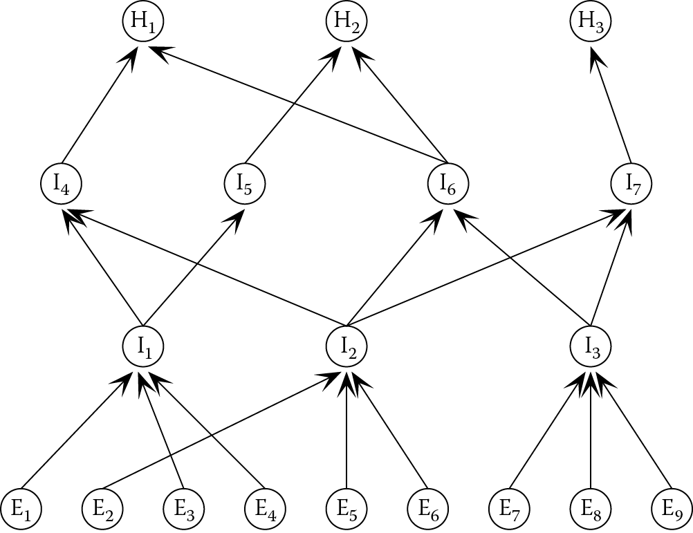
A deeper Bayesian inference network (Ei = evidence, Hi = hypothesis, Ii = intermediate hypothesis).

In contrast, the inference network in Figure 3.4 includes several intermediate steps. The probabilities at each node are modified as the reasoning process proceeds, until they reach their final values. Note that the rules in the boiler control example made use of several intermediate nodes that helped to make the rules more understandable and avoided duplication of tests for specific pieces of evidence.
In order to maintain some consistency of rule format, the condition parts of rule r3_1 given earlier have been joined by a conjunction (and). However, the formal treatment of Bayesian updating allows no distinction between conjoining (and) and disjoining (or) evidence. Instead, each item of evidence is assumed to contribute independently toward updating the probability of the hypothesis (i.e., the conclusion).
3.2.7 Combining Bayesian Rules with Production Rules
In a practical rule-based system, we may wish to mix uncertain rules with production rules. For instance, we may wish to make use of the following production rule even though the assertion release_valve is stuck may have been established with a probability less than 1.
rule r3_1a
if release_valve is stuck
then task becomes clean_release_valve.
In this case, the hypothesis that the release valve needs cleaning can be asserted with the same probability as the evidence. This avoids the issue of providing a prior probability for the hypothesis or a weighting for the evidence.
If a production rule contains multiple pieces of evidence that are independent from each other, their combined probability can be derived from standard probability theory. Consider, for example, a rule in which two pieces of independent evidence are conjoined (i.e., they are joined by and):
if <evidence E1> and <evidence E2> then <hypothesis H3>.
The probability of hypothesis H3 is given by
P(H3) = P(E1) × P(E2) (3.25)
Production rules containing independent evidence that is disjoined (i.e., joined by or) can be treated in a similar way. So given the rule
if <evidence E1> or <evidence E2> then <hypothesis H3>.
the probability of hypothesis H3 is given by
P(H3) = P(E1) + P(E2) – (P(E1) × P(E2)) (3.26)
The Flint toolkit (Beaudoin et al. 2005) takes a different approach in which the production rules are treated as though they were Bayesian. A default prior probability of 0.5 is assigned to the hypothesis, and the weighted affirms and denies weights, A′ and D′, are assumed to equal the odds of the evidence, O(E). This approach is equivalent to the method described earlier if there is only one item of evidence, but deviates from it for multiple items of evidence.
3.2.8 A Worked Example of Bayesian Updating
We will consider the same example that was introduced in Chapter 2, namely, control of a power station boiler. Let us start with just four rules in Flex format:
rule r3_1a
if release_valve is stuck
then task becomes clean_release_valve.
rule r3_2a
if warning_light is on
then release_valve becomes stuck.
rule r3_3a
if pressure is high
then release_valve becomes stuck.
rule r3_4a
if temperature is high
and water_level is not low
then pressure becomes high.
The conclusion of each of these rules is expressed as an assertion. The four rules contain four assertions (or hypotheses) and three pieces of evidence that are independent of the rules, namely, the temperature, the status of the warning light (on or off), and the water level. The various probability estimates for these and their associated affirms and denies weights are shown in Table 3.1.
Values Used in the Worked Example of Bayesian Updating
|
H |
E |
P(H) |
O(H) |
P(E|H) |
P(E|~H) |
A |
D |
|
release valve needs cleaning |
release valve is stuck |
— |
— |
— |
— |
— |
— |
|
release valve is stuck |
warning light is on |
0.02 |
0.02 |
0.88 |
0.4 |
2.20 |
0.20 |
|
release valve is stuck |
pressure is high |
0.02 |
0.02 |
0.85 |
0.01 |
85.0 |
0.15 |
|
pressure is high |
temperature is high |
0.1 |
0.11 |
0.90 |
0.05 |
18.0 |
0.11 |
|
pressure is high |
water level is low |
0.1 |
0.11 |
0.05 |
0.5 |
0.10 |
1.90 |
Having calculated the affirms and denies weights, we can now rewrite our production rules as probabilistic rules. We will leave the first rule as a production rule, albeit in the altered format of Flint, in order to illustrate the interaction between production rules and probabilistic rules. Our new rule set is therefore as follows:
uncertainty_rule r3_1b
if release_valve is stuck
then task becomes clean_release_valve.
uncertainty_rule r3_2b
if warning_light is on (affirms 2.20; denies 0.20)
then release_valve becomes stuck.
uncertainty_rule r3_3b
if pressure is high (affirms 85.0; denies 0.15)
then release_valve becomes stuck.
uncertainty_rule r3_4b
if temperature is high (affirms 18.0; denies 0.11)
and water_level is low (affirms 0.10; denies 1.90)
then pressure becomes high.
Rule r3_4b makes use of two pieces of evidence, and it no longer needs a negative condition, as this has been accommodated by the affirms and denies weights. The requirement that water_level is not low be supportive evidence is expressed by the denies weight of water_level is low being greater than 1 while the affirms weight is less than 1.
To illustrate how the various weights are used, let us consider how a Bayesian inference engine would use the following set of input data:
water_level is not low.
warning light is on.
temperature is high.
We will assume that the rules fire in the following order:
r3_4b → r3_3b → r3_2b → r3_1b
The resultant rule trace might then appear as follows:
uncertainty_rule r3_4b
H = pressure is high; O(H) = 0.11
E1 = temperature is high; A1 = 18.0
E2 = water_level is low; D2 = 1.90
O(H|(E1&~E2)) = O(H) × A1 × D2 = 3.76
/* Updated odds of "pressure is high" are 3.76 */
uncertainty_rule r3_3b
H = release_valve is stuck; O(H) = 0.02
E = pressure is high; A = 85.0
Because E is not certain (O(E) = 3.76, P(E) = 0.79), the inference engine must calculate an interpolated value A' for the affirms weight of E (see Section 3.2.5).
A'= [2(A-1) × P(E)] + 2 - A = 49.7
O(H|(E)) = O(H) × A' = 0.99
/* Updated odds of "release_valve is stuck" are 0.99, */
/* corresponding to a probability of approximately 0.5 */
uncertainty_rule r3_2b
H = release_valve is stuck; O(H) = 0.99
E = warning_light is on; A = 2.20
O(H|(E)) = O(H) × A = 2.18
/* Updated odds of "release_valve is stuck" are 2.18 */
uncertainty_rule r3_1b
H = task is clean_release_valve
E = release_valve is stuck;
O(E)= 2.18 implies O(H)= 2.18
/* This is a production rule, so the conclusion is asserted with the same probability as the evidence. */
/* Updated odds of "task is clean_release_valve" are 2.18 */
3.2.9 Discussion of the Worked Example
The foregoing example serves to illustrate a number of features of Bayesian updating. Our final conclusion that the release valve needs cleaning is reached with a certainty represented as
O(task is clean_release_valve) = 2.18
or
P(task is clean_release_valve) = 0.69
Thus, there is a probability of 0.69 that the valve needs cleaning. In a real-world situation, this is a more realistic outcome than concluding that the valve definitely needs cleaning, which would have been the conclusion had we used the original set of production rules.
The initial three items of evidence were all stated with complete certainty: water level is not low; warning_light is on; and temperature is high. These are given facts, and P(E) = 1 for each of them. Consider the evidence warning_light is on. A probability of less than 1 might be associated with this evidence if it were generated as an assertion by another probabilistic rule, or if it were supplied as an input to the system, but the user’s view of the warning light was impaired. If P(warning light is on) is 0.8, an interpolated value of the affirms weight would be used in rule r3_2b. Equation 3.16 yields an interpolated value of 1.72 for the affirms weight.
However, if P(warning light is on) were less than 0.5, then an interpolated denies weighting would be used. If P(warning light is on) were 0.3, an interpolated denies weighting of 0.68 is yielded by Equation 3.17.
If P(warning light is on) = 0.5, then the warning light is just as likely to be on as it is to be off. If we try to interpolate either the affirms or denies weight, a value of 1 will be found. Thus, if each item of evidence for a particular rule has a probability of 0.5, then the rule has no effect whatsoever.
Assuming that the prior probability of a hypothesis is less than 1 and greater than 0, the hypothesis can never be confirmed with complete certainty by the application of likelihood ratios, as this would require its odds to become infinite.
While Bayesian updating is a mathematically rigorous technique for updating probabilities, it is important to remember that the results obtained can only be valid if the data supplied are valid. This is the key issue to consider when assessing the virtues of the technique. The probabilities shown in Table 3.1 have not been measured from a series of trials, but instead, they are an expert’s best guesses. Given that the values upon which the affirms and denies weights are based are only guesses, then a reasonable alternative to calculating them is to simply take an educated guess at the appropriate weightings. Such an approach is just as valid or invalid as calculating values from unreliable data. If a rule-writer takes such an ad hoc approach, the provision of both an affirms and denies weighting becomes optional. If an affirms weight is provided for a piece of evidence E, but not a denies weight, then that rule can be ignored when P(E) < 0.5.
As well as relying on the rule-writer’s weightings, Bayesian updating is also critically dependent on the values of the prior probabilities. Obtaining accurate estimates for these is also problematic.
Even if we assume that all of the data supplied in the foregoing worked example are accurate, the validity of the final conclusion relies upon the statistical independence from each other of the supporting pieces of evidence. In our example, as with very many real problems, this assumption is dubious. For example, pressure is high and warning_light is on were used as independent pieces of evidence, when in reality there is a cause-and-effect relationship between the two.
3.2.10 Advantages and Disadvantages of Bayesian Updating
Bayesian updating is a means of handling uncertainty by updating the probability of an assertion when evidence for or against the assertion is provided. The principal advantages of Bayesian updating are
- The technique is based upon a proven statistical theorem.
- Likelihood is expressed as a probability (or odds), which has a clearly defined and familiar meaning.
- The technique requires deductive probabilities, which are generally easier to estimate than abductive ones. The user supplies values for the probability of evidence (the symptoms) given a hypothesis (the cause), rather than the reverse.
- Likelihood ratios and prior probabilities can be replaced by sensible guesses. This is at the expense of advantage (1), as the probabilities subsequently calculated cannot be interpreted literally but rather as an imprecise measure of likelihood.
- Evidence for and against a hypothesis (or the presence and absence of evidence) can be combined in a single rule by using affirms and denies weights.
- Linear interpolation of the likelihood ratios can be used to take account of any uncertainty in the evidence (i.e., uncertainty about whether the condition part of the rule is satisfied), although this is an ad hoc solution.
- The probability of a hypothesis can be updated in response to more than one piece of evidence.
The principal disadvantages of Bayesian updating are
- The prior probability of an assertion must be known or guessed at.
- Conditional probabilities must be measured or estimated or, failing those, guesses must be taken at suitable likelihood ratios. Although the conditional probabilities are often easier to judge than the prior probability, they are nevertheless a considerable source of errors. Estimates of likelihood are often clouded by a subjective view of the importance or utility of a piece of information (Buchanan and Duda 1983).
- The single probability value for the truth of an assertion tells us nothing about its precision.
- Because evidence for and against an assertion are lumped together, no record is kept of how much there is of each.
- The addition of a new rule that asserts a new hypothesis often requires alterations to the prior probabilities and weightings of several other rules. This contravenes one of the main advantages of knowledge-based systems.
- The assumption that pieces of evidence are independent is often unfounded. The only alternatives are to calculate affirms and denies weights for all possible combinations of dependent evidence, or to restructure the rule base so as to minimize these interactions.
- The linear interpolation technique for dealing with uncertain evidence is not mathematically justified.
- Representations based on odds, as required to make use of likelihood ratios, cannot handle absolute truth, that is, odds = ∞.
3.3 Certainty Theory
3.3.1 Introduction
Certainty theory (Shortliffe and Buchanan 1975), sometimes called Stanford certainty theory, is an adaptation of Bayesian updating that is incorporated into the EMYCIN expert system shell. EMYCIN is based on MYCIN (Shortliffe 1976), an expert system that assists in the diagnosis of infectious diseases. The name EMYCIN is derived from “essential MYCIN,” reflecting the fact that it is not specific to medical diagnosis and that its handling of uncertainty is simplified. Certainty theory represents an attempt to overcome some of the shortcomings of Bayesian updating, although the mathematical rigor of Bayesian updating is lost. As this rigor is rarely justified by the quality of the data, the loss of rigor may not be a significant problem.
3.3.2 Making Uncertain Hypotheses
Instead of using probabilities, each assertion in EMYCIN has a certainty value associated with it. Certainty values can range between 1 and –1.
For a given hypothesis H, its certainty value C(H) is given by
C(H) = 1.0 if H is known to be true;
C(H) = 0.0 if H is unknown;
C(H) = –1.0 if H is known to be false.
There is a similarity between certainty values and probabilities, such that
C(H) = 1.0 corresponds to P(H) = 1.0;
C(H) = 0.0 corresponds to P(H) being at its a priori value;
C(H) = –1.0 corresponds to P(H) = 0.0.
Each rule also has a certainty associated with it, known as its certainty factor, CF. Certainty factors serve a similar role to the affirms and denies weightings in Bayesian systems:
uncertainty_rule generic1
if <evidence>
then <hypothesis>
with certainty factor <CF>.
Part of the simplicity of certainty theory stems from the fact that identical measures of certainty are attached to rules and hypotheses. The certainty factor of a rule is modified to reflect the level of certainty of the evidence, such that the modified certainty factor CF′ is given by
(3.27)
If the evidence is known to be present, that is, C(E) = 1, then Equation 3.27 yields CF′ = CF.
The technique for updating the certainty of hypothesis H, in the light of evidence E, involves the application of the following composite function:
(3.28)
(3.29)
(3.30)
where
C(H|E) is the certainty of H updated in the light of evidence E;
C(H) is the initial certainty of H, that is, 0, unless it has been updated by the previous application of a rule;
|x| is the magnitude of x, that is, ignoring its sign.
It can be seen from the foregoing equations that the updating procedure consists of adding a positive or negative value to the current certainty of a hypothesis. This contrasts with Bayesian updating where the odds of a hypothesis are multiplied by the appropriate likelihood ratio. The composite function represented by Equations 3.28 to 3.30 is plotted in Figure 3.5 and can be seen to have a broadly similar shape to the Bayesian updating equation (plotted in Figure 3.1).

In the standard version of certainty theory, a rule can only be applied if the certainty of the evidence C(E) is greater than 0, that is, if the evidence is more likely to be present than not. EMYCIN restricts rule-firing further by requiring that C(E) > 0.2 for a rule to be considered applicable. The justification for this heuristic is that it saves computational power and makes explanations clearer, as marginally effective rules are suppressed. In fact, it is possible to allow rules to fire regardless of the value of C(E). The absence of supporting evidence, indicated by C(E) < 0, would then be taken into account since CF′ would have the opposite sign from CF.
Although there is no theoretical justification for the function for updating certainty values, it does have a number of desirable properties:
- The function is continuous and has no singularities or steps.
- The updated certainty C(H|E) always lies within the bounds −1 and +1.
- If either C(H) or CF′ is +1 (i.e., definitely true), then C(H|E) is also +1.
- If either C(H) or CF′ is −1 (i.e., definitely false), then C(H|E) is also −1.
- When contradictory conclusions are combined, they tend to cancel each other out, that is, if C(H) = − CF′, then C(H|E) = 0.
- Several pieces of independent evidence can be combined by repeated application of the function, and the outcome is independent of the order in which the pieces of evidence are applied.
- If C(H) = 0, that is, the certainty of H is at its a priori value, then C(H|E) = CF′.
- If the evidence is certain (i.e., C(E) = 1), then CF′ = CF.
- Although not part of the standard implementation, the absence of evidence can be taken into account by allowing rules to fire when C(E) < 0.
3.3.3 Logical Combinations of Evidence
In Bayesian updating systems, each piece of evidence that contributes toward a hypothesis is assumed to be independent and is given its own affirms and denies weights. In systems based upon certainty theory, the certainty factor is associated with the rule as a whole rather than with individual pieces of evidence. For this reason, certainty theory provides a simple algorithm for determining the value of the certainty factor that should be applied when more than one item of evidence is included in a single rule. The relationship between pieces of evidence is made explicit by the use of and and or. If separate pieces of evidence are intended to contribute toward a single hypothesis independently of each other, they must be placed in separate rules. The algorithm for combining items of evidence in a single rule is borrowed from Zadeh’s possibility theory (Section 3.4). The algorithm covers the cases where evidence is conjoined (i.e., joined by and), disjoined (i.e., joined by or), and negated (using not).
3.3.3.1 Conjunction
Consider a rule of the form
uncertainty_rule generic2
if <evidence E1>
and <evidence E2>
then <hypothesis>
with certainty factor <CF>.
The certainty of the combined evidence is given by C(E1 and E2), where
C(E1 and E2) = min[C(E1), C(E2)] (3.31)
3.3.3.2 Disjunction
Consider a rule of the form
uncertainty_rule generic3
if <evidence E1>
or <evidence E2>
then <hypothesis>
with certainty factor <CF>.
The certainty of the combined evidence is given by C(E1 or E2), where
C(E1 or E2) = max[C(E1), C(E2)] (3.32)
3.3.3.3 Negation
Consider a rule of the form
uncertainty_rule generic4
if not <evidence E>
then <hypothesis>
with certainty factor <CF>.
The certainty of the negated evidence, C(E), is given by C(~E), where
C(~E) = –C(E) (3.33)
3.3.4 A Worked Example of Certainty Theory
In order to illustrate the application of certainty theory, we can rework the example that was used to illustrate Bayesian updating. Four rules were used, which together could determine whether the release valve of a power station boiler needs cleaning (see Section 3.2.8). Each of the four rules can be rewritten with an associated certainty factor, which is estimated by the rule-writer:
uncertainty_rule r3_1c
if release_valve is stuck
then task becomes clean_release_valve
with certainty factor 1.0.
uncertainty_rule r3_2c
if warning_light is on
then release_valve becomes stuck
with certainty factor 0.2.
uncertainty_rule r3_3c
if pressure is high
then release_valve becomes stuck
with certainty factor 0.9.
uncertainty_rule r3_4c
if temperature is high
and water_level is not low
then pressure becomes high
with certainty factor 0.5.
Although the process of providing certainty factors might appear ad hoc compared with Bayesian updating, it may be no less reliable than estimating the probabilities upon which Bayesian updating relies. In the Bayesian example, the production rule r3_1b had to be treated as a special case. In a system based upon uncertainty theory, rule r3_1c can be made to behave as a production rule simply by giving it a certainty factor of 1.
As before, the following set of input data will be considered:
water_level is not low.
warning_light is on.
temperature is high.
We will assume that the rules fire in the order
r3_4c → r3_3c → r3_2c → r3_1c
The resultant rule trace might then appear as follows:
uncertainty_rule r3_4c CF = 0.5
H = pressure is high; C(H) = 0
E1 = temperature is high; C(E1) = 1
E2 = water_level is low; C(E2) = -1, C(~E2) = 1
C(E1&~E2) = min[C(E1),C(~E2)] = 1
CF' = CF × C(E1&~E2) = CF
C(H|(E1&~E2)) = CF' = 0.5
/* Updated certainty of "pressure is high" is 0.5 */
uncertainty_rule r3_3c CF = 0.9
H = release_valve is stuck; C(H) = 0
E = pressure is high; C(E) = 0.5
CF' = CF × C(E) = 0.45
C(H|(E)) = CF' = 0.45
/* Updated certainty of "release_valve is stuck" is 0.45 */
uncertainty_rule r3_2c CF = 0.2
H = release_valve is stuck; C(H) = 0.45
E = warning_light is on; C(E) = 1
CF' = CF × C(E) = CF
C(H|(E)) = C(H) + [CF' × (1-C(H))] = 0.56
/* Updated certainty of "release_valve is stuck" is 0.56 */
uncertainty_rule r3_1c CF = 1
H = task is clean_release_valve C(H) = 0
E = release_valve is stuck; C(E) = 0.56
CF' = CF × C(E) = 0.56
C(H|(E)) = CF' = 0.56
/* Updated certainty of "task is clean_release_valve" is 0.56 */
3.3.5 Discussion of the Worked Example
Given the certainty factors shown, the example yielded the result that the release valve needs cleaning with a similar level of confidence to the Bayesian updating example.
Under Bayesian updating, rules r3_2b and r3_3b could be combined into a single rule without changing their effect:
uncertainty_rule r3_5b
if warning_light is on (affirms 2.20; denies 0.20)
and pressure is high (affirms 85.0; denies 0.15)
then release_valve becomes stuck.
With certainty theory, the weightings apply not to the individual pieces of evidence (as with Bayesian updating) but to the rule itself. If rules r3_2c and r3_3c were combined in one rule, a single certainty factor would need to be chosen to replace the two used previously. Thus a combined rule might look like
uncertainty_rule r3_5c
if warning_light is on
and pressure is high
then release_valve becomes stuck
with certainty factor 0.95.
In the combined rule, the two items of evidence are no longer treated independently, and the certainty factor is the adjudged weighting if both items of evidence are present. If our worked example had contained this combined rule instead of rules r3_2c and r3_3c, then the rule trace would contain the following:
uncertainty_rule r3_5c CF = 0.95
H = release_valve is stuck; C(H) = 0
E1 = warning_light is on; C(E1) = 1
E2 = pressure is high; C(E2) = 0.5
C(E1 & E2) = min[C(E1),C(E2)] = 0.5
CF' = CF × C(E1 & E2) = 0.48
C(H|(E1 & E2)) = CF' = 0.48
/* Updated certainty of "release_valve is stuck" is 0.48 */
With the certainty factors used in the example, the combined rule yields a lower confidence in the hypothesis release_valve is stuck than rules r3_2c and r3_3c used separately. As a knock-on result, rule r3_1c would yield the conclusion task is clean_release_valve with a diminished certainty of 0.48.
3.3.6 Relating Certainty Factors to Probabilities
It has already been noted that there is a similarity between the certainty factors that are attached to hypotheses and the probabilities of those hypotheses, such that
C(H) = 1.0 corresponds to P(H) = 1.0;
C(H) = 0.0 corresponds to P(H) being at its a priori value;
C(H) = –1.0 corresponds to P(H) = 0.0.
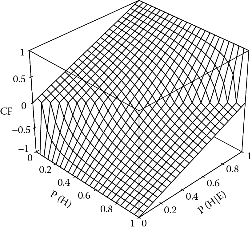
Additionally, a formal relationship exists between the certainty factor associated with a rule and the conditional probability P(H|E) of a hypothesis H given some evidence E. This is only of passing interest as certainty factors are not normally calculated in this way but instead are simply estimated or chosen to give suitable results. The formal relationships are as follows.
If evidence E supports hypothesis H, that is, P(H|E) is greater than P(H), then
(3.34)
If evidence E opposes hypothesis H, that is, P(H|E) is less than P(H), then
(3.35)
The shape of Equations 3.34 and 3.35 is shown in Figure 3.6.
3.4 Fuzzy Logic: Type-1
Bayesian updating and certainty theory are techniques for handling the uncertainty that arises, or is assumed to arise, from statistical variations or randomness. Fuzzy logic, sometimes called possibility theory, addresses a different source of uncertainty, namely, vagueness in the use of language. Fuzzy logic was developed by Zadeh (1975, 1983a, 1983b) and builds upon his theory of fuzzy sets (Zadeh 1965). Zadeh asserts that, while probability theory may be appropriate for measuring the likelihood of a hypothesis, it says nothing about the meaning of the hypothesis. A goal of fuzzy logic is to achieve “computing with words” (Zadeh 1996). This section focuses on the simplest and most commonly used form of fuzzy logic, known as type-1. Section 3.6 discusses a more sophisticated form of fuzzy logic, known as type-2.
3.4.1 Crisp Sets and Fuzzy Sets
The rules shown in this chapter and in Chapter 2 contain a number of examples of vague language where fuzzy sets might be applied, such as the following phrases:
- Water level is low.
- Temperature is high.
- Pressure is high.
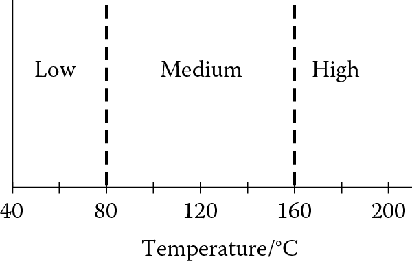
In conventional set theory, the sets high, medium, and low—applied to a variable such as temperature—would be mutually exclusive. If a given temperature (say, 200°C) is high, then it is neither medium nor low. Such sets are said to be crisp or nonfuzzy (Figure 3.7). If the boundary between medium and high is set at 160°C, then a temperature of 161°C is considered high, while 159°C is considered medium. This distinction is rather artificial and means that a tiny difference in temperature can completely change the rule-firing, while a rise in temperature from 161°C to 300°C has no effect at all.
Fuzzy sets are a means of smoothing out the boundaries. The theory of fuzzy sets expresses imprecision quantitatively by introducing characteristic membership functions that can assume values between 0 and 1 corresponding to degrees of membership from “not a member” through to “a full member.” If F is a fuzzy set, then the membership function µF (x) measures the degree to which an absolute value x belongs to F. This degree of membership is sometimes called the possibility that x is described by F. The process of deriving these possibility values for a given value of x is called fuzzification.
Conversely, consider that we are given the imprecise statement temperature is low. If LT is the fuzzy set of low temperatures, then we might define the membership function µLT such that
µLT (140°C) = 0.0
µLT (120°C) = 0.0
µLT (100°C) = 0.25
µLT (80°C) = 0.5
µLT (60°C) = 0.75
µLT (40°C) = 1.0
µLT (20°C) = 1.0
These values correspond with the linear membership function shown in Figure 3.8. Although linear membership functions like those in Figures 3.8a,b are convenient in many applications, the most suitable shape of the membership functions and the number of fuzzy sets depends on the particular application. Figures 3.8c,d show some nonlinear alternatives.

The key differences between fuzzy and crisp sets are that
- an element has a degree of membership [0–1] of a fuzzy set;
- membership of one fuzzy set does not preclude membership of another.
Thus, the temperature 180°C may have some (nonzero) degree of membership to both fuzzy sets high and medium. This is represented in Figure 3.8 by the overlap between the fuzzy sets. The sum of the membership functions for a given value can be arranged to equal 1, as shown for temperature and pressure in Figure 3.8, but this is not a necessary requirement.
Some of the terminology of fuzzy sets may require clarification. The statement temperature is low is an example of a fuzzy statement involving a fuzzy set (low temperature) and a fuzzy variable (temperature). A fuzzy variable is one that can take any value from a global set (e.g., the set of all temperatures), where each value can have a degree of membership of a fuzzy set (e.g., low temperature) associated with it.
Although the discussion so far has concentrated on continuous variables such as temperature and pressure, the same ideas can also be applied to discrete variables, such as the number of signals detected in a given time span.
3.4.2 Fuzzy Rules
If a variable is set to a value by crisp rules, its value will change in steps as different rules fire. The only way to smooth those steps would be to have a large number of rules. However, only a small number of fuzzy rules are required to produce smooth changes in the outputs as the input values alter. The number of fuzzy rules required is dependent on the number of variables, the number of fuzzy sets, and the ways in which the variables are combined in the fuzzy rule conditions. Numerical information is explicit in crisp rules, for example, “if temperature > 160°C then …” but in fuzzy rules it becomes implicit in the chosen shape of the fuzzy membership functions.
Consider a rule base that contains the following fuzzy rules:
fuzzy_rule r3_6f
if temperature is high
then pressure becomes high.
fuzzy_rule r3_7f
if temperature is medium
then pressure becomes medium.
fuzzy_rule r3_8f
if temperature is low
then pressure becomes low.
Suppose the measured boiler temperature is 180°C. As this is a member of both fuzzy sets high and medium, rules r3_6f and r3_7f will both fire. The pressure, we conclude, will be somewhat high and somewhat medium. Suppose that the membership functions for temperature are as shown in Figure 3.8. The possibility that the temperature is high, µHT, is 0.75, and the possibility that the temperature is medium, µMT, is 0.25. As a result of firing the rules, the possibilities that the pressure is high and medium, µHP and µMP, are set as follows:
µHP = max[µHT , µHP]
µMP = max[µMT , µMP]
The initial possibility values for pressure are assumed to be zero if these are the first rules to fire, and thus µHP and µMP become 0.75 and 0.25, respectively. These values can be passed on to other rules that might have pressure is high or pressure is medium in their condition clauses.
The rules r3_6f, r3_7f, and r3_8f contain only simple conditions. Possibility theory provides a recipe for computing the possibilities of compound conditions. The formulas for conjunction, disjunction, and negation are similar to those used in certainty theory (Section 3.3.3):
(3.36)
To illustrate the use of these formulas, suppose that water level has the fuzzy membership functions shown in Figure 3.8 and that rule r3_6f is redefined as follows:
fuzzy_rule r3_9f
if temperature is high
and water_level is not low
then pressure becomes high.
For a water level of 1.2 m, the possibility of the water level being low, µLW, is 0.6. The possibility of the water level not being low is therefore 0.4. As this is less than 0.75, the combined possibility for the temperature being high and the water level not being low is 0.4. Thus the possibility that the pressure is high, µHP, becomes 0.4 if it has not already been set to a higher value.
If several rules affect the same fuzzy set of the same variable, they are equivalent to a single rule whose conditions are joined by the disjunction or. For example, these two rules
fuzzy_rule r3_6f
if temperature is high
then pressure becomes high.
fuzzy_rule r3_10f
if water_level is high
then pressure becomes high.
are equivalent to this single rule:
fuzzy_rule r3_11f
if temperature is high
or water_level is high
then pressure becomes high.
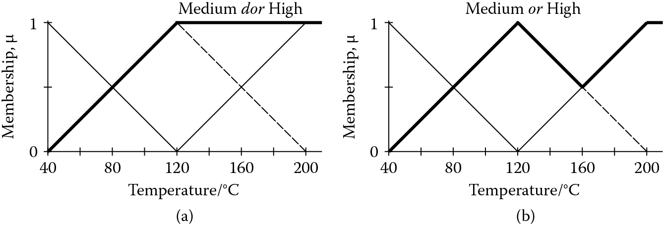
Aoki and Sasaki (Aoki and Sasaki 1990) have argued for treating the disjunction or differently when it involves two fuzzy sets of the same fuzzy variable, for example, high and medium temperature. In such cases, the memberships are clearly dependent on each other. Therefore, we can introduce a new operator dor for “dependent or.” For example, given the rule
fuzzy_rule r3_12f
if temperature is low
dor temperature is medium
then pressure becomes lowish.
the combined possibility for the condition becomes
(3.37)
Given the fuzzy sets for temperature shown in Figure 3.8, the combined possibility would be the same for any temperature below 120°C, as shown in Figure 3.9. This is consistent with the intended meaning of fuzzy rule r3_12f. If the or operator had been used, the membership would dip between 40°C and 120°C, with a minimum at 80°C, as shown in Figure 3.9.
3.4.3 Defuzzification
In the foregoing example, at a temperature of 180°C, the possibilities for the pressure being high and medium, µHP and µMP, are set to 0.75 and 0.25, respectively, by the fuzzy rules r3_6f and r3_7f. It is assumed that the possibility for the pressure being low, µLP, remains at 0. These values can be passed on to other rules that might have pressure is high or pressure is medium in their condition clauses without any further manipulation. However, if we want to interpret these membership values in terms of a numerical value of pressure, they would need to be defuzzified. Defuzzification is particularly important when the fuzzy variable is a control action such as “set current,” where a specific setting is required. The use of fuzzy logic in control systems is discussed further in Section 3.5. Defuzzification takes place in two stages, described in the following text.
3.4.3.1 Stage 1: Scaling the Membership Functions
The first step in defuzzification is to adjust the fuzzy sets in accordance with the calculated possibilities. A commonly used method is Larsen’s product operation rule (Lee 1990a, 1990b), in which the membership functions are multiplied by their respective possibility values. The effect is to compress the fuzzy sets so that the peaks equal the calculated possibility values, as shown in Figure 3.10. Some authors (Johnson and Picton 1995) adopt an alternative approach in which the fuzzy sets are truncated, as shown in Figure 3.11. For most shapes of fuzzy set, the difference between the two approaches is small, but Larsen’s product operation rule has the advantages of simplifying the calculations and allowing fuzzification followed by defuzzification to return the initial value, except as described in the subsection “A defuzzification anomaly” in the following text.

Larsen’s product operation rule for calculating membership functions from fuzzy rules. Membership functions for pressure are shown, derived from Rules 3.6f and 3.7f, for a temperature of 180°C.

Truncation method for calculating membership functions from fuzzy rules. Membership functions for pressure are shown, derived from Rules 3.6f and 3.7f, for a temperature of 180°C.
3.4.3.2 Stage 2: Finding the Centroid
The most commonly used method of defuzzification is the centroid method, sometimes called the center of gravity, center of mass, or center of area method. Defuzzification by determining the centroid of the fuzzy output function is part of an overall process known as Mamdani-style fuzzy inference (Mamdani 1977). The defuzzified value is taken as the point along the fuzzy variable axis that is the centroid, or balance point, of all the scaled membership functions taken together for that variable (Figure 3.12). One way to visualize this is to imagine the membership functions cut out from stiff card and pasted together where (and if) they overlap. The defuzzified value is the balance point along the fuzzy variable axis of this composite shape. When two membership functions overlap, both overlapping regions contribute to the mass of the composite shape. Figure 3.12 shows a simple case, involving neither the low nor high fuzzy sets. The example that we have been following concerning boiler pressure is more complex and is described in Section 3.4.3.3 in the following text.

If there are N membership functions with centroids ci and areas ai, then the combined centroid C, that is, the defuzzified value, is
(3.38)
When the fuzzy sets are compressed using Larsen’s product operation rule, the values of ci are unchanged from the centroids of the uncompressed shapes, Ci, and ai is simply μiAi, where Ai is the area of the membership function prior to compression. (This is not the case with the truncation method shown in Figure 3.11, which causes the centroid of asymmetrical membership functions to shift along the fuzzy variable axis.) The use of triangular membership functions or other simple geometries simplifies the calculations further. For triangular membership functions, Ai is one half of the base length multiplied by the height. For isosceles triangles, Ci is the midpoint along the base, and for right-angle triangles, Ci is approximately 29% of the base length from the upright.
3.4.3.3 Defuzzifying at the Extremes
There is a complication in defuzzifying whenever the two extreme membership functions are involved, that is, those labeled high and low here. Given the fuzzy sets shown in Figure 3.8, any pressure above 0.7 MNm−2 has a membership of high of 1. Thus the membership function continues indefinitely toward the right, and we cannot find a balance point using the centroid method. Similarly, any pressure below 0.1 MNm−2 has a membership of low of 1, although in this case the membership function is bounded because the pressure cannot go below 0.
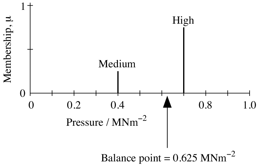
One solution to these problems might be to specify a range for the fuzzy variable, MIN–MAX, or 0.1–0.7 MNm−2 in this example. During fuzzification, a value outside this range can be accepted and given a membership of 1 for the fuzzy sets low or high. However, during defuzzification, the low and high fuzzy sets can be considered bounded at MIN and MAX, and defuzzification by the centroid method can proceed. This method is shown in Figure 3.13 using the values 0.75 and 0.25 for µHP and µMP, respectively, as calculated in Section 3.4.2, yielding a defuzzified pressure of 0.527 MNm−2. A drawback of this solution is that the defuzzified value can never reach the extremes of the range. For example, if we know that a fuzzy variable has a membership of 1 for the fuzzy set high and 0 for the other fuzzy sets, then its actual value could be any value greater than or equal to MAX. However, its defuzzified value using this scheme would be the centroid of the high fuzzy set, in this case 0.612 MNm−2, which is considerably below MAX.

An alternative solution is the mirror rule. During defuzzification only, the low and high membership functions are treated as symmetrical shapes centered on MIN and MAX, respectively. This is achieved by reflecting the low and high fuzzy sets in imaginary mirrors. This method has been used in Figure 3.13, yielding a significantly different result, that is, 0.625 MNm−2, for the same possibility values. The method uses the full range MIN–MAX of the fuzzy variable during defuzzification so that a fuzzy variable with a membership of 1 for the fuzzy set high and 0 for the other fuzzy sets would be defuzzified to MAX.
3.4.3.4 Sugeno Defuzzification
So far we have considered defuzzification by determining the centroid of the fuzzy output function, that is, the Mamdani method (Mamdani 1977). As the output may be a combination of several scaled membership functions, determination of the centroid can become computationally expensive. However, the combination of four assumptions can greatly simplify the defuzzification calculation:
- Larsen’s product operation rule is applied.
- The mirror rule is applied.
- The membership functions for the output are symmetrical (after applying the mirror rule, if required, at the extremes).
- The membership functions for the output have the same area Ai (prior to compression through Larsen’s product operation rule).
When all four assumptions are made, the calculation of the centroid of the fuzzy output function becomes equivalent to determining the weighted average of a set of singletons, that is, spike functions, as shown in Figure 3.14. With the introduction of this simplification of the defuzzification calculation, the whole process is known as zero-order Sugeno fuzzy inference (Takagi and Sugeno 1985). The height of each spike is the same as the height of the corresponding fuzzy output in a Mamdani-style system. The centroid, that is, the weighted sum of the singletons, is given by
(3.39)
where each value of μi is the height of spike i, and Ci is its position along the fuzzy-variable axis (Hopgood et al. 1998). Equation 3.39 represents a considerable simplification of the more general equation for defuzzification shown in Equation 3.38.
3.4.3.5 A Defuzzification Anomaly
It is interesting to investigate whether defuzzification can be regarded as the inverse of fuzzification. In the foregoing example, a pressure of 0.625 MNm−2 would fuzzify to a membership of 0.25 for medium and 0.75 for high. When defuzzified by the method shown in Figure 3.13, the original value of 0.625 MNm−2 is returned. This observation provides strong support for defuzzification based upon Larsen’s product operation rule combined with the mirror rule for dealing with the fuzzy sets at the extremes (Figure 3.13). No such simple relationship exists if the membership functions are truncated (Figure 3.11) instead of being compressed Larsen’s product operation rule, or if the extremes are handled by imposing a range (Figure 3.13) instead of applying the mirror rule.
However, even the full set of four assumptions listed earlier for zero-order Sugeno fuzzy inference cannot always guarantee that fuzzification and defuzzification will be straightforward inverses of each other. For example, as a result of firing a set of fuzzy rules, we might end up with the following memberships for the fuzzy variable pressure:
- Low membership = 0.25
- Medium membership = 0.0
- High membership = 0.25
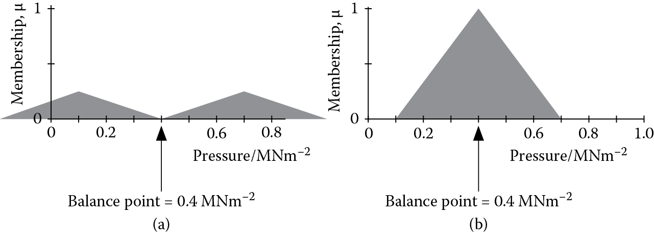
Defuzzification of these membership values would yield an absolute value of 0.4 MNm−2 for the pressure (Figure 3.15). If we were now to look up the fuzzy memberships for an absolute value of 0.4 MNm−2, that is, to fuzzify the value, we would obtain
- Low membership = 0.0
- Medium membership = 1.0
- High membership = 0.0
The resulting membership values are clearly different from the ones we started with, although they still defuzzify to 0.4 MNm−2, as shown in Figure 3.15. The reason for this anomaly is that, under defuzzification, there are many different combinations of membership values that can yield an absolute value such as 0.4 MNm−2. The foregoing sets of membership values are just two examples. However, under fuzzification, there is only one absolute value, namely 0.4 MNm−2, that can yield fuzzy membership values for low, medium, and high of 0.0, 1.0, and 0.0, respectively. Thus, defuzzification is said to be a “many-to-one” relationship, whereas fuzzification is a “one-to-one” relationship.
This observation poses a dilemma for implementers of a fuzzy system. If pressure appears in the condition part of further fuzzy rules, different membership values could be used depending on whether or not it is defuzzified and refuzzified before being passed on to those rules.
A secondary aspect of the anomaly is the observation that, in the foregoing example, we began with possibility values of 0.25 and, therefore, apparently rather weak evidence about the pressure. However, as a result of defuzzification followed by fuzzification, these values are transformed into evidence that appears much stronger. Johnson and Picton (Johnson and Picton 1995) have labeled this “Hopgood’s defuzzification paradox.” The paradox arises because, unlike probabilities or certainty factors, possibility values need to be interpreted relative to each other rather than in absolute terms.
3.5 Fuzzy Control Systems
3.5.1 Crisp and Fuzzy Control
Control decisions can be thought of as a transformation from state variables to action variables (Figure 3.16). State variables describe the current state of the physical plant and the desired state. Action variables are those that can be directly altered by the controller, such as the electrical current sent to a furnace, or the flow rate through a gas valve. In some circumstances, it may be possible to obtain values for the action variables by direct mathematical manipulation of the state variables. This is the case for a PID (proportional + integral + derivative) controller—see Chapter 14, Section 14.2.5. Given suitably chosen functions, this mathematical modeling approach causes values of action variables to change smoothly as values of state variables change. However, in high-level control, such as, for a complex manufacturing process, analytical functions that link state variables to action variables are rarely available. This is one reason for using rules instead for this purpose.

Crisp sets are conventional Boolean sets where an item is either a member (degree of membership = 1) or it is not (degree of membership = 0). Applying crisp sets to state and action variables corresponds to dividing up the range of allowable values into subranges, each of which forms a set. Suppose that a state variable such as temperature is divided into five crisp sets. A temperature reading can belong to only one of these sets, so only one rule will apply, resulting in a single control action. Thus, the number of different control actions is limited to the number of rules, which in turn is limited by the number of crisp sets. The action variables are changed in abrupt steps as the state variables change.
Fuzzy logic enables a small number of rules to produce smooth changes in the action variables as the state variables change. It is, therefore, particularly well suited to control decisions where the control actions need to be scaled as input measurements change. The number of rules required is dependent on the number of state variables, the number of fuzzy sets, and the ways in which the state variables are combined in rule conditions. Numerical information is explicit in crisp rules, but in fuzzy rules it becomes implicit in the chosen shape of the fuzzy membership functions.
3.5.2 Fuzzy Control Rules
Some simple examples of fuzzy control rules for an industrial electric oven are as follows:
fuzzy_rule r3_13f
if temperature is high
or current is high
then current_change becomes reduce.
fuzzy_rule r3_14f
if temperature is medium
then current_change becomes no_change.
fuzzy_rule r3_15f
if temperature is low
and current is high
then current_change becomes no_change.
fuzzy_rule r3_16f
if temperature is low
and current is low
then current_change becomes increase.
The rules and the fuzzy sets to which they refer are, in general, dependent on each other. Figure 3.17 shows some possible fuzzy membership functions, µ, for the state variables temperature and current, and for the required change in current, that is, for the action variable current_change. The state variables are the inputs to the fuzzy controller, and the action variable is the output. Since the fuzzy sets overlap, a temperature and current may have a nonzero degree of membership of more than one fuzzy set. Some variation in the shapes of the fuzzy sets has been introduced in this example so that the sum of the memberships for a particular fuzzy variable is not necessarily equal to 1. Suppose that the recorded temperature is 300°C and the measured current is 15 A. The temperature and current are each members of two fuzzy sets: medium and high. Rules r3_13f and r3_14f will fire, with the apparently contradictory conclusion that we should both reduce the electric current and leave it alone. Of course, what is actually required is some reduction in current.

Fuzzy sets: (a) electric current (state variable), (b) temperature (state variable), (c) change in electric current (action variable).
Rule r3_13f contains a disjunction. Using Equation 3.36, the possibility value for the composite condition is
max(µ(temperature is high), µ(current is high)).
At 300°C and 15 A, µ(temperature is high) is 0.3 and µ(current is high) is 0.5. The composite possibility value is therefore 0.5, and µ(current_change is reduce) becomes 0.5. Rule r3_14f is simpler, containing only a single condition. The possibility value µ(temperature is medium) is 0.3, and so µ(current_change is no_change) becomes 0.3.
3.5.3 Defuzzification in Control Systems
After firing rules r3_13f and r3_14f, current_change has a degree of membership, or possibility, for reduce and another for no_change. These fuzzy actions must be converted into a single precise action to be of any practical use, that is, they need to be defuzzified.
Assuming that we are using Larsen’s Product Operation Rule (see Section 3.4.3), the membership functions for the control actions are compressed according to their degree of membership. Thus, the membership functions for reduce and for no_change are compressed so that their peak values become 0.5 and 0.3, respectively (Figure 3.18). Defuzzification can then take place by finding the centroid of the combined membership functions.

One of the membership functions, that is, reduce, covers an extremity of the fuzzy variable current_change and, therefore, continues indefinitely toward −∞. As discussed in Section 3.4.3, a method of handling this is required in order to find the centroid. Figure 3.19 shows the effect of applying the mirror rule so that the membership function for reduce is treated, for defuzzification purposes only, as though it were symmetrical around −50%.

As the initial membership functions for the output, current_change, are symmetrical (after applying the mirror rule) and they have the same area, all of the assumptions for zero-order Sugeno fuzzy inference are now satisfied. So, the centroid C is given by
(3.39)
Inserting the values from Figure 3.18, we obtain
(3.40)
Thus, the defuzzified control action is a 31.25% reduction in the current, as shown in Figure 3.19.
3.6 Fuzzy Logic: Type-2
While type-1 fuzzy logic is undoubtedly useful, as demonstrated by its numerous applications in control systems and elsewhere, it is sometimes criticized for being too precise in its handling of membership functions. Since a given value of a variable, such as temperature, has a fixed membership value of a fuzzy set such as low, it might be argued that there is no uncertainty at all. This weakness was recognized by the architect of fuzzy logic himself, Zadeh, in his pioneering paper (Zadeh 1975). To overcome this perceived weakness, he proposed that the membership of a fuzzy set could itself be treated as a fuzzy variable. The result is a “fuzzy-fuzzy” model, known as type-2 fuzzy logic. In principle, there is no need to stop there. The second-order membership could also be a fuzzy variable, resulting in type-3 fuzzy logic. The concept can be generalized to type-n fuzzy logic, although types 1 and 2 dominate current research and practice.
In the example considered in Figure 3.8, a temperature such as 60°C has the following memberships of the type-1 fuzzy sets low, medium, and high:
µLT (60°C) = 0.75
µMT (60°C) = 0.25
µHT (60°C) = 0
This model successfully accommodates the use of vague language in the sense that words such as “low” and “medium” can represent a range of different temperatures with differing levels of membership. What it does not allow, however, are differing interpretations of the words “low” and “medium.” So, what we really need, and type-2 fuzzy logic provides, is a way to represent the idea that µLT (60°C) is “about 0.75,” and µMT (60°C) is “about 0.25.”
Mendel (Mendel 2007) describes an experiment where 50 people are asked to define the endpoints of a description such as “low temperature.” (His example describes levels of eye contact, but the principle is the same.) In the context of an industrial boiler, the upper bound of “low temperature” might be set by such a sample of people to fall in the range 60°C–130°C, with a mean of 95°C. A type-1 fuzzy set could be constructed using the mean value, but this would not reflect the spread of opinion about how to interpret the phrase “low temperature” in this context. In particular, it would fail to recognize that a large proportion of the sample think that, in this context, “low temperature” can be above the boiling point of water at atmospheric pressure. (In the example used in Section 3.4, the upper bound for “low temperature” was actually set at 120°C.)
In order to model such a spread of opinion in type-2 fuzzy logic, we need to recognize the existence of a continuum of alternative fuzzy sets whose endpoints are in the specified range. The boundaries of the fuzzy set are no longer a line of infinitesimal thickness but a band known as the footprint of uncertainty. Then, if we were to look up the membership of “low temperature” for a specific temperature such as 80°C, we would not find just a single membership value, as in a type-1 fuzzy set, but a range of possibilities from within the footprint of uncertainty. Values in this range might all be considered equally likely, in which case the fuzzy set is said to be interval type-2 (Figure 3.20). Alternatively, a weighting function known as the secondary membership function, z, can be imposed so that, for example, values close to the mean might be weighted most highly. The latter fuzzy sets are generalized type-2 (Figure 3.20). Interval type-2 fuzzy sets grew in popularity quite rapidly because of their computational simplicity, but generalized type-2 are now starting to take centre stage owing to their greater expressiveness (John and Coupland 2007). The secondary membership functions for type-1, interval type-2, and generalized type-2 fuzzy sets are compared in Figure 3.21.
(a) 
(b) 
Type-2 fuzzy sets: (a) interval, (b) generalized. (Derived from Wagner, C., and H. Hagras. 2010.)
(a) 
(b) 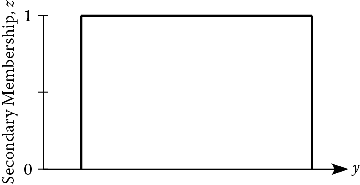
(c) 
Secondary membership functions for (a) type-1 fuzzy set, (b) interval type-2 fuzzy set, and (c) generalized type-2 fuzzy set. (Derived from Wagner, C., and H. Hagras. 2010.)
3.7 Other Techniques
Fuzzy logic, or possibility theory, occupies a distinct position among the many strategies for handling uncertainty, as it is the only established one that is concerned specifically with uncertainty arising from imprecise use of language. Techniques have been developed for dealing with other specific sources of uncertainty. For example, plausibility theory (Rescher 1976) addresses the problems arising from unreliable or contradictory sources of information. Other techniques have been developed in order to overcome some of the perceived shortcomings of Bayesian updating and certainty theory. Notable among these are the Dempster–Shafer theory of evidence and Quinlan’s Inferno, both of which are briefly reviewed here.
None of the more specialized techniques for handling uncertainty overcomes the most difficult problem, namely, obtaining accurate estimates of the likelihood of events and combinations of events. For this reason, their use may be difficult to justify in many practical knowledge-based systems.
3.7.1 Dempster–Shafer Theory of Evidence
The theory of evidence (Barnett 1981) is a generalization of probability theory that was created by Dempster and developed by Shafer (Shafer 1976). It addresses two specific deficiencies of probability theory that have already been highlighted, namely, that
- the single probability value for the truth of a hypothesis tells us nothing about its precision;
- because evidence for and against a hypothesis are lumped together, we have no record of how much there is of each.
Rather than representing the probability of a hypothesis H by a single value P(H), Dempster and Shafer’s technique binds the probability to a subinterval L(H)–U(H) of the range 0–1. Although the exact probability P(H) may not be known, L(H) and U(H) represent lower and upper bounds on the probability such that
L(H) ≤ P(H) ≤ U(H) (3.41)
The precision of our knowledge about H is characterized by the difference U(H)–L(H). If this is small, our knowledge about H is fairly precise, but if it is large, we know relatively little about H. A clear distinction is therefore made between uncertainty and ignorance, where uncertainty is expressed by the limits on the value of P(H), and ignorance is represented by the size of the interval defined by those limits. According to Buchanan and Duda (Buchanan and Duda 1983), Dempster and Shafer have pointed out that the Bayesian agony of assigning prior probabilities to hypotheses is often due to ignorance of the correct values, and this ignorance can make any particular choice arbitrary and unjustifiable.
The foregoing ordering (3.41) can be interpreted as two assertions:
- The probability of H is at least L(H).
- The probability of ~H is at least 1.0 – U(H).
Thus, a separate record is kept of degree of belief and disbelief in H. Like Bayesian updating, the theory of evidence benefits from the solid basis of probability theory for the interpretation of L(H) and U(H). When L(H) = U(H), the theory of evidence reduces to the Bayesian updating method. It is, therefore, not surprising that the theory of evidence also suffers from many of the same difficulties.
3.7.2 Inferno
The conclusions that can be reached by the Dempster–Shafer theory of evidence are of necessity weaker than those that can be arrived at by Bayesian updating. If the available knowledge does not justify stronger solutions, then drawing weaker solutions is desirable. This theme is developed further in Inferno (Quinlan 1983), a technique that its creator, Quinlan, has subtitled “a cautious approach to uncertain inference.” Although Inferno is based upon probability theory, it avoids assumptions about the dependence or independence of pieces of evidence and hypotheses. As a result, the correctness of any inferences can be guaranteed, given the available knowledge. Thus, Inferno deliberately errs on the side of caution.
The three key motivations for the development of Inferno were as follows:
- Other systems often make unjustified assumptions about the dependence or independence of pieces of evidence or hypotheses. Inferno allows users to state any such relationships when they are known, but it makes no assumptions.
- Other systems take a measure of belief (e.g., probability or certainty) in a piece of evidence and calculate from it a measure of belief in a hypothesis or conclusion. In terms of a Bayesian inference network (Figure 3.3 and Figure 3.4), probabilities or certainty values are always propagated in one direction, namely, from the bottom (evidence) to the top (conclusions). Inferno allows users to enter values for any node on the inference network and to observe the effects on values at all other nodes.
- Inferno informs the user of inconsistencies that might be present in the information presented to it and can make suggestions of ways to restore consistency.
Quinlan (Quinlan 1983) gives a detailed account of how these aims are achieved, and provides a comprehensive set of expressions for propagating probabilities throughout the nodes of an inference network.
3.8 Summary
A number of different schemes exist for assigning numerical values to assertions in order to represent levels of confidence in them and for updating the confidence levels in the light of supporting or opposing evidence. The greatest difficulty lies in obtaining accurate values of likelihood, whether measured as a probability or by some other means. The certainty factors that are associated with rules in certainty theory, and the affirms and denies weightings in Bayesian updating, can be derived from probability estimates. However, a more pragmatic approach is frequently adopted, namely, to choose values that produce the right sort of results, even though the values cannot be theoretically justified. As the more sophisticated techniques (e.g., Dempster–Shafer theory of evidence and Inferno) also depend upon probability estimates that are often dubious, their use may be difficult to justify.
Bayesian updating is soundly based on probability theory, whereas many of the alternative techniques are ad hoc. In practice, Bayesian updating is also an ad hoc technique because
- linear interpolation of the affirms and denies weighting is frequently used as a convenient means of compensating for uncertainty in the evidence;
- the likelihood ratios (or the probabilities from which they are derived) and prior probabilities are often based on estimates rather than statistical analysis;
- separate items of evidence that support a single assertion are assumed to be statistically independent, although this may not be the case in reality.
Neural networks (see Chapter 8) represent an alternative approach that avoids the difficulties in obtaining reliable probability estimates. Neural networks can be used to train a computer system using many examples so that it can draw conclusions weighted according to the evidence supplied. Of course, given a large enough set of examples, it would also be possible to calculate accurately the prior probabilities and weightings needed in order to make Bayesian updating or one of its derivatives work effectively.
Fuzzy logic is also closely associated with neural networks, as will be discussed in Chapter 9. Fuzzy logic provides a precise way of handling vague terms such as “low” and “high” using fuzzy sets. Type-2 fuzzy logic takes this vagueness a stage further by allowing uncertainty in the membership functions that describe the fuzzy sets. Fuzzy logic enables a small set of rules to produce output values that change smoothly as the input values change. Fuzzy controllers exploit this characteristic by ensuring that deviations in the state variables of the controlled system are remedied by appropriately scaled control actions.
Further Reading
Bouchon-Meunier, B., C. Marsala, M. Rifqi, and R. R. Yager, eds. 2008. Uncertainty and Intelligent Information Systems. World Scientific, Hong Kong.
Hajek, P., T. Havranek, and R. Jirousek. 1992. Uncertain Information Processing in Expert Systems. CRC Press, Boca Raton, FL.
Jantzen, J. 2007. Foundations of Fuzzy Control. Wiley-Blackwell, London.
Kandel, A. 1991. Fuzzy Expert Systems. CRC Press, Boca Raton, FL.
Klir, G. J., and M. J. Wierman. 2010. Uncertainty-Based Information: Elements of Generalized Information Theory (Studies in Fuzziness and Soft Computing). 2nd ed. Physica-Verlag, Heidelberg.
Li, H. X., and V. C. Yen. 1995. Fuzzy Sets and Fuzzy Decision-Making. CRC Press, Boca Raton, FL.
Ross, T. J. 2010. Fuzzy Logic with Engineering Applications. 3rd ed. Wiley-Blackwell, London.