When we introduced random-number generation, we mentioned that if the random module’s randrange function indeed produces integers at random, then every number in the specified range has an equal probability (or likelihood) of being chosen each time the function is called. For a six-sided die, each value 1 through 6 should occur one-sixth of the time, so the probability of any one of these values occurring is 1/6_th or about 16.667%.

In the next section, we create and execute a dynamic (that is, animated) die-rolling simulation script. In general, you’ll see that the more rolls we attempt, the closer each die value’s percentage of the total rolls gets to 16.667% and the heights of the bars gradually become about the same. This is a manifestation of the law of large numbers.

FuncAnimation drives a frame-by-frame animation. Each animation frame specifies everything that should change during one plot update. Stringing together many of these updates over time creates the animation effect. You decide what each frame displays with a function you define and pass to FuncAnimation.

Each animation frame will:

• roll the dice a specified number of times (from 1 to as many as you’d like), updating die frequencies with each roll,

• clear the current plot,

• create a new set of bars representing the updated frequencies, and

• create new frequency and percentage text for each bar.

Generally, displaying more frames-per-second yields smoother animation. For example, video games with fast-moving elements try to display at least 30 frames-per-second and often more. Though you’ll specify the number of milliseconds between animation frames, the actual number of frames-per-second can be affected by the amount of work you perform in each frame and the speed of your computer’s processor. This example displays an animation frame every 33 milliseconds—yielding approximately 30 (1000 / 33) frames-per-second. Try larger and smaller values to see how they affect the animation. Experimentation is important in developing the best visualizations.

In the previous chapter’s Intro to Data Science section, we developed the static visualization interactively so you could see how the code updates the bar plot as you execute each statement. The actual bar plot with the final frequencies and percentages was drawn only once.

For this dynamic visualization, the screen results update frequently so that you can see the animation. Many things change continuously—the lengths of the bars, the frequencies and percentages above the bars, the spacing and labels on the axes and the total number of die rolls shown in the plot’s title. For this reason, we present this visualization as a script, rather than interactively developing it.

The script takes two command-line arguments:

• number_of_frames—The number of animation frames to display. This value determines the total number of times that FuncAnimation updates the graph. For each animation frame, FuncAnimation calls a function that you define (in this example, update) to specify how to change the plot.

• rolls_per_frame—The number of times to roll the die in each animation frame. We’ll use a loop to roll the die this number of times, summarize the results, then update the graph with bars and text representing the new frequencies.

To understand how we use these two values, consider the following command:

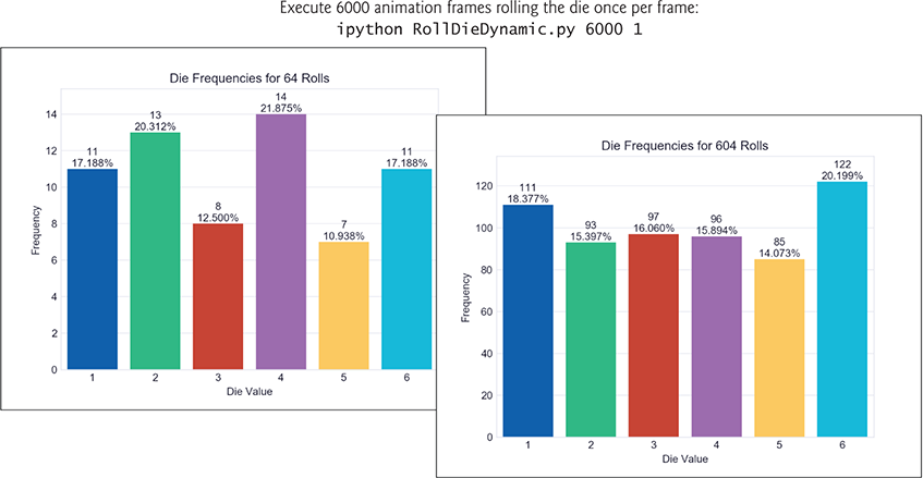
ipython RollDieDynamic.py 6000 1

In this case, FuncAnimation calls our update function 6000 times, rolling one die per frame for a total of 6000 rolls. This enables you to see the bars, frequencies and percentages update one roll at a time. On our system, this animation took about 3.33 minutes (6000 frames / 30 frames-per-second / 60 seconds-per-minute) to show you only 6000 die rolls.

Displaying animation frames to the screen is a relatively slow input–output-bound operation compared to the die rolls, which occur at the computer’s super fast CPU speeds. If we roll only one die per animation frame, we won’t be able to run a large number of rolls in a reasonable amount of time. Also, for small numbers of rolls, you’re unlikely to see the die percentages converge on their expected 16.667% of the total rolls.

To see the law of large numbers in action, you can increase the execution speed by rolling the die more times per animation frame. Consider the following command:

ipython RollDieDynamic.py 10000 600

In this case, FuncAnimation will call our update function 10,000 times, performing 600 rolls-per-frame for a total of 6,000,000 rolls. On our system, this took about 5.55 minutes (10,000 frames / 30 frames-per-second / 60 seconds-per-minute), but displayed approximately 18,000 rolls-per-second (30 frames-per-second * 600 rolls-per-frame), so we could quickly see the frequencies and percentages converge on their expected values of about 1,000,000 rolls per face and 16.667% per face.

Experiment with the numbers of rolls and frames until you feel that the program is helping you visualize the results most effectively. It’s fun and informative to watch it run and to tweak it until you’re satisfied with the animation quality.

We took the following four screen captures during each of two sample executions. In the first, the screens show the graph after just 64 die rolls, then again after 604 of the 6000 total die rolls. Run this script live to see over time how the bars update dynamically. In the second execution, the screen captures show the graph after 7200 die rolls and again after 166,200 out of the 6,000,000 rolls. With more rolls, you can see the percentages closing in on their expected values of 16.667% as predicted by the law of large numbers.

We focus primarily on the new features used in this example. Line 3 imports the Matplotlib animation module.

1 # RollDieDynamic.py
2 """Dynamically graphing frequencies of die rolls."""
3 from matplotlib import animation
4 import matplotlib.pyplot as plt
5 import random
6 import seaborn as sns
7 import sys
8

Lines 9–27 define the update function that FuncAnimation calls once per animation frame. This function must provide at least one argument. Lines 9–10 show the beginning of the function definition. The parameters are:

• frame_number—The next value from FuncAnimation’s frames argument, which we’ll discuss momentarily. Though FuncAnimation requires the update function to have this parameter, we do not use it in this update function.

• rolls—The number of die rolls per animation frame.

• faces—The die face values used as labels along the graph’s x-axis.

• frequencies—The list in which we summarize the die frequencies.

We discuss the rest of the function’s body in the next several subsections.

 9 def update(frame_number, rolls, faces, frequencies):
10     """Configures bar plot contents for each animation frame."""

Lines 12–13 roll the die rolls times and increment the appropriate frequencies element for each roll. Note that we subtract 1 from the die value (1 through 6) before incrementing the corresponding frequencies element—as you’ll see, frequencies is a six-element list (defined in line 36), so its indices are 0 through 5.

11    # roll die and update frequencies
12    for i in range(rolls):
13        frequencies[random.randrange(1, 7) - 1] += 1
14

Line 16 in function update calls the matplotlib.pyplot module’s cla (clear axes) function to remove the existing bar plot elements before drawing new ones for the current animation frame. We discussed the code in lines 17–27 in the previous chapter’s Intro to Data Science section. Lines 17–20 create the bars, set the bar plot’s title, set the x- and y-axis labels and scale the plot to make room for the frequency and percentage text above each bar. Lines 23–27 display the frequency and percentage text.

15     # reconfigure plot for updated die frequencies
16     plt.cla() # clear old contents contents of current Figure
17     axes = sns.barplot(faces, frequencies, palette='bright') # new bars
18     axes.set_title(f'Die Frequencies for {sum(frequencies):,} Rolls')
19     axes.set(xlabel='Die Value', ylabel='Frequency')
20     axes.set_ylim(top=max(frequencies) * 1.10) # scale y-axis by 10%
21
22     # display frequency & percentage above each patch (bar)
23     for bar, frequency in zip(axes.patches, frequencies):
24         text_x = bar.get_x() + bar.get_width() / 2.0
25         text_y = bar.get_height()
26         text = f'{frequency:,}
{frequency / sum(frequencies):.3%}'
27         axes.text(text_x, text_y, text, ha='center', va='bottom')
28

Lines 30 and 31 use the sys module’s argv list to get the script’s command-line arguments. Line 33 specifies the Seaborn 'whitegrid' style. Line 34 calls the matplotlib.pyplot module’s figure function to get the Figure object in which FuncAnimation displays the animation. The function’s argument is the window’s title. As you’ll soon see, this is one of FuncAnimation’s required arguments. Line 35 creates a list containing the die face values 1–6 to display on the plot’s x-axis. Line 36 creates the six-element frequencies list with each element initialized to 0—we update this list’s counts with each die roll.

29 # read command-line arguments for number of frames and rolls per frame
30 number_of_frames = int(sys.argv[1])
31 rolls_per_frame = int(sys.argv[2])
32
33 sns.set_style('whitegrid') # white background with gray grid lines
34 figure = plt.figure('Rolling a Six-Sided Die') # Figure for animation
35 values = list(range(1, 7)) # die faces for display on x-axis
36 frequencies = [0] * 6 # six-element list of die frequencies
37

Lines 39–41 call the Matplotlib animation module’s FuncAnimation function to update the bar chart dynamically. The function returns an object representing the animation. Though this is not used explicitly, you must store the reference to the animation; otherwise, Python immediately terminates the animation and returns its memory to the system.

38 # configure and start animation that calls function update
39 die_animation = animation.FuncAnimation(
40     figure, update, repeat=False, frames=number_of_frames, interval=33,
41     fargs=(rolls_per_frame, values, frequencies))
42
43 plt.show() # display window

FuncAnimation has two required arguments:

• figure—the Figure object in which to display the animation, and

• update—the function to call once per animation frame.

In this case, we also pass the following optional keyword arguments:

• repeat—False terminates the animation after the specified number of frames. If True (the default), when the animation completes it restarts from the beginning.

• frames—The total number of animation frames, which controls how many times FunctAnimation calls update. Passing an integer is equivalent to passing a range—for example, 600 means range(600). FuncAnimation passes one value from this range as the first argument in each call to update.

• interval—The number of milliseconds (33, in this case) between animation frames (the default is 200). After each call to update, FuncAnimation waits 33 milliseconds before making the next call.

• fargs (short for “function arguments”)—A tuple of other arguments to pass to the function you specified in FuncAnimation’s second argument. The arguments you specify in the fargs tuple correspond to update’s parameters rolls, faces and frequencies (line 9).

For a list of FuncAnimation’s other optional arguments, see

https://matplotlib.org/api/_as_gen/matplotlib.animation.FuncAnimation.html

Finally, line 43 displays the window.