9.1 (Class Average: Writing Grades to a Plain Text File) Figure 3.2 presented a class-average script in which you could enter any number of grades followed by a sentinel value, then calculate the class average. Another approach would be to read the grades from a file. In an IPython session, write code that enables you to store any number of grades into a grades.txt plain text file.

9.2 (Class Average: Reading Grades from a Plain Text File) In an IPython session, write code that reads the grades from the grades.txt file you created in the previous exercise. Display the individual grades and their total, count and average.

9.3 (Class Average: Writing Student Records to a CSV File) An instructor teaches a class in which each student takes three exams. The instructor would like to store this information in a file named grades.csv for later use. Write code that enables an instructor to enter each student’s first name and last name as strings and the student’s three exam grades as integers. Use the csv module to write each record into the grades.csv file. Each record should be a single line of text in the following CSV format:

9.4 (Class Average: Reading Student Records from a CSV File) Use the csv module to read the grades.csv file from the previous exercise. Display the data in tabular format.

9.5 (Class Average: Creating a Grade Report from a CSV File) Modify your solution to the preceding exercise to create a grade report that displays each student’s average to the right of that student’s row and the class average for each exam below that exam’s column.

9.6 (Class Average: Writing a Gradebook Dictionary to a JSON File) Reimplement Exercise 9.3 using the json module to write the student information to the file in JSON format. For this exercise, create a dictionary of student data in the following format:

9.7 (Class Average: Reading a Gradebook Dictionary from a JSON File) Reimplement Exercise 9.4 using the json module to read the grades.json file created in the previous exercise. Display the data in tabular format, including an additional column showing each student’s average to the right of that student’s three exam grades and an additional row showing the class average on each exam below that exam’s column.

9.8 (pickle Object Serialization and Deserialization) We mentioned that we prefer to use JSON for object serialization due to the Python documentation’s stern security warnings about pickle. However, pickle has been used to serialize objects for many years, so you’re likely to encounter it in Python legacy code. According to the documentation, “If you are doing your own pickle writing and reading, you’re safe (provided no one else has access to the pickle file, of course.)”¹⁴ Reimplement your solutions to Exercises 9.6–9.7 using the pickle module’s dump function to serialize the dictionary into a file and its load function to deserialize the object. Pickle is a binary format, so this exercise requires binary files. Use the file-open mode 'wb' to open the binary file for writing and 'rb' to open the binary file for reading. Function dump receives as arguments an object to serialize and a file object in which to write the serialized object. Function load receives the file object containing the serialized data and returns the original object. The Python documentation suggests the pickle file extension .p.

9.9 (Telephone-Number Word Generator) In Exercise 5.12, you created a telephone-number word-generator program. Modify that program to write its output to a text file.

9.10 (Project: Analyzing a Book from Project Gutenberg) A great source of plain text files is the collection of over 57,000 free e-books at Project Gutenberg:

9.11 (Project: Visualizing Word Frequencies with a Word Cloud) A word cloud visualizes words, displaying more frequently occurring words in larger fonts. In this exercise, you’ll create a word cloud that visualizes the top 200 words in Pride and Prejudice. You’ll use the open-source wordcloud module’s¹⁵ WordCloud class to generate a word cloud with just a few lines of code.

9.12 (Project: State-of-the-Union Speeches) Text files of all U.S. Presidents’ State-of-the-Union speeches are available online. Download one of these speeches. Write a script that reads the speech from the file, then displays statistics about the speech, including the total word count, the total character count, the average word length, the average sentence length, a word distribution of the words frequencies, and the top 10 longest words. In the “Natural Language Processing (NLP)” chapter, you’ll find lots of more sophisticated techniques for analyzing and comparing such texts.

9.13 (Project: Building a Basic Sentiment Analyzer) We’ll do lots of sentiment analysis in the data-science chapters. For example, we’ll look at large numbers of tweets from Twitter on various topics, determining whether people had positive or negative opinions about those topics. We’ll see that many software packages have built-in sentiment-analysis capabilities. In this exercise, you’ll build a basic sentiment analyzer. A basic way to do this is to search online for files of positive words (like happy, pleasant, …) and files of negative words (like sad, angry, …). Then, search through a text to see how many positive words and how many negative words it contains. Based on those counts, rate the text as positive, negative or neutral.

9.14 (Project: Basic Similarity Detection via Average Sentence Length and Average Word Length) Who actually wrote William Shakespeare’s works? Some researchers believe that Sir Francis Bacon may have authored some or all of these works. Download one of Shakespeare’s works and one of Bacon’s works from Project Gutenberg. For each, calculate the average sentence length and average word length. Are these close? Compute other statistics as well.

9.15 (Project: Working with CSV Datasets Using the csv Module) In the Intro to Data Science section, we loaded the Titanic disaster dataset into a pandas DataFrame, then used DataFrame capabilities to perform some simple analysis of that data. For this exercise, use the csv module to read the Titanic disaster dataset, then manually count the records that contain a value for the age column. Those that do not will have the value 'NA'. For only those records that have an age value, calculate the average age. For this exercise, investigate and use the csv module’s DictReader class.

9.16 (Working with the diamonds.csv Dataset in Pandas) In this book’s data-science chapters, you’ll work extensively with datasets, many in CSV format. You’ll frequently use pandas to load datasets and prepare their data for use in machine-learning studies. Datasets are available for almost anything you’d want to study. There are numerous dataset repositories from which you can download datasets in CSV and other formats. In this chapter, we mentioned:

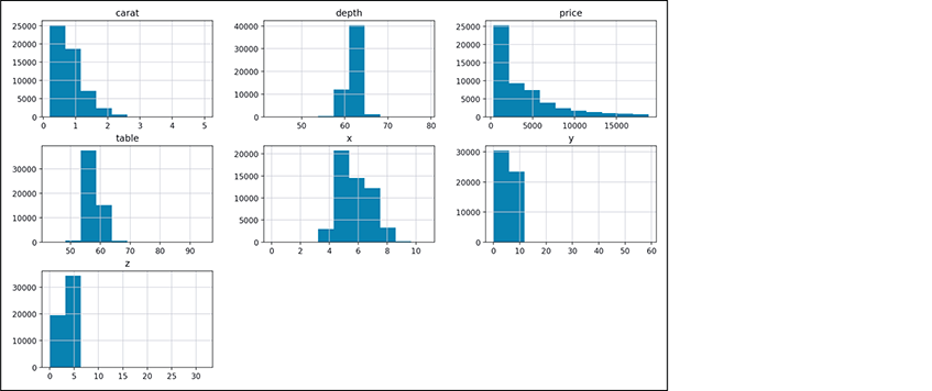
9.17 (Working with the Iris.csv Dataset in Pandas) Another popular dataset for machine-learning novices is the Iris dataset, which contains 150 records of information about three Iris plant species. Like this diamonds dataset, the Iris dataset is available from various online sources, including Kaggle. Investigate the Iris dataset’s columns,¹⁸ then perform the following tasks to study and analyze the dataset:

9.18 (Project: Anscombe’s Quartet CSV) Locate a CSV file online containing the data for Anscombe’s Quartet. Load the data into a pandas DataFrame. Investigate pandas built-in scatter-plot capability for plotting x-y coordinate pairs and use it to plot the x-y coordinate pairs in Anscombe’s Quartet.

9.19 (Challenging Project: A Crossword-Puzzle Generator) Most people have worked crossword puzzles, but few have ever attempted to generate one by hand. Generating a crossword puzzle is suggested here as a string-manipulation and file-processing project requiring substantial sophistication and effort.

9.20 (Challenging Project: A Spell Checker) Many apps you use daily have built-in spell checkers. In the “Natural Language Processing,” “Machine Learning” and “Deep Learning” chapters, you’ll learn techniques that can be used to build sophisticated spell checkers. In this project, you’ll take a simpler, more mechanical approach. You’ll need a computerized dictionary as a source of words.