
Appendices
The set ![]() of real numbers has deficiencies. For example, the equation x2 + 1 = 0 has no real root; that is, no real number u exists such that u2 + 1 = 0. This type of problem also exists for the set
of real numbers has deficiencies. For example, the equation x2 + 1 = 0 has no real root; that is, no real number u exists such that u2 + 1 = 0. This type of problem also exists for the set ![]() of natural numbers. It contains no solution of the equation x + 1 = 0, and the set
of natural numbers. It contains no solution of the equation x + 1 = 0, and the set ![]() of integers was invented to solve such equations. But
of integers was invented to solve such equations. But ![]() is also inadequate (for example, 2x − 1 = 0 has no root in
is also inadequate (for example, 2x − 1 = 0 has no root in ![]() ), and hence the set
), and hence the set ![]() of rational numbers was invented. Again,
of rational numbers was invented. Again, ![]() contains no solution to x2 − 2 = 0, so the set
contains no solution to x2 − 2 = 0, so the set ![]() of real numbers was created. Similarly, the set
of real numbers was created. Similarly, the set ![]() of complex numbers was invented that contains a root of x2 + 1 = 0. More precisely, there is a complex number i such that
of complex numbers was invented that contains a root of x2 + 1 = 0. More precisely, there is a complex number i such that
i2 = − 1.
However, the process ends here. The complex numbers have the property that every nonconstant polynomial with complex coefficients has a (complex) root. In 1799, at the age of 22, Carl Friedrich Gauss first proved this result, which is known as the Fundamental Theorem of Algebra. We give a proof in Section 6.6.
In this appendix, we describe the set ![]() of complex numbers. The set of real numbers is usually identified with the set of all points on a straight line. Similarly, the complex numbers are identified with the points in the euclidean plane by labeling the point with cartesian coordinates (a, b) as
of complex numbers. The set of real numbers is usually identified with the set of all points on a straight line. Similarly, the complex numbers are identified with the points in the euclidean plane by labeling the point with cartesian coordinates (a, b) as
(a, b) = a + bi.
Then the set ![]() of complex numbers is defined by
of complex numbers is defined by
![]()
When this is done, the resulting Euclidean plane is called the complex plane.
Each real number a is identified with the point a = a + 0i = (a, 0) on the x-axis in the usual way, and for this reason the x-axis is called the real axis. The points
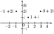
bi = 0 + bi = (0, b) on the y-axis are called imaginary numbers, and the y-axis is called the imaginary axis.138 The diagram shows the complex plane and several complex numbers.
Identification of the complex number a + bi = (a, b) with the ordered pair (a, b) immediately gives the following condition for equality:
Equality Principle. a = bi = a′ + b′ i if and only if a = a′ and b = b′.
For a complex number z = a + bi, the real numbers a and b are called the real part of z and the imaginary part of z, respectively, and are denoted by a = rez and b = imz. Hence, the equality principle becomes as follows: Two complex numbers are equal if and only if their real parts are equal and their imaginary parts are equal.
With the requirement that i2 = − 1, we define addition and multiplication of complex numbers as follows:
![]()
These operations are analogous to those for linear polynomials a + bx, with one difference: i2 = − 1. These definitions imply that complex numbers satisfy all the arithmetic axioms enjoyed by real numbers. Hence, they may be manipulated in the obvious fashion, except that we replace i2 by −1 whenever it occurs.
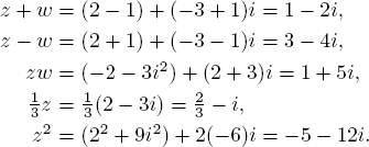
Example 1. If z = 2 − 3i and ![]()
Example 2. Find all complex numbers z such that z2 = − i.
Solution. Write z = a + bi, where a and b are to be determined. Then the condition z2 = − i becomes
(a2 − b2) + 2abi = 0 + (− 1)i.
Equating real and imaginary parts gives a2 = b2 and 2ab = − 1. The solution is
![]()
Theorem 1 collects the basic properties of addition and multiplication of complex numbers. The verifications are straightforward and left to the reader.
Theorem 1. If z, u, and ![]() are complex numbers, then
are complex numbers, then

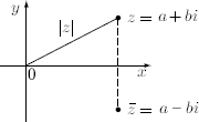
The following two notions are indispensable when working with complex numbers. If z = a + bi is a complex number, the conjugate ![]() and the absolute value (or modulus) |z| are defined by
and the absolute value (or modulus) |z| are defined by
![]()
Thus, ![]() is a complex number and is the reflec-tion of z in the real axis (see the diagram), whereas |z| is a nonnegative real number and equals the distance between z and the origin. Note that the absolute value of a real number a = a + 0i is
is a complex number and is the reflec-tion of z in the real axis (see the diagram), whereas |z| is a nonnegative real number and equals the distance between z and the origin. Note that the absolute value of a real number a = a + 0i is ![]() using the definition of absolute value for complex num-bers, which agrees with the absolute value of a regarded as a real number.
using the definition of absolute value for complex num-bers, which agrees with the absolute value of a regarded as a real number.
Theorem 2. Let z and ![]() denote complex numbers. Then
denote complex numbers. Then
1. ![]()
2. ![]()
3. ![]()
4. z is real if and only if ![]()
5. ![]()
6. |z| ≥ 0 and |z| = 0 if and only if z = 0
7. ![]()
Proof. (1) We prove (2), (5), and (7) and leave the rest to the reader. If z = a + bi and ![]() we compute
we compute

which proves (2). Next, (5) follows from
![]()
Finally (2) and (5) give
![]()
Then (7) follows when we take positive square roots.
Let z be a nonzero complex number. Then (6) of Theorem 2 shows that |z| ≠ 0, and so ![]() by (5). As a result, we call the complex number
by (5). As a result, we call the complex number ![]() the inverse of z and denote it z−1 = 1/z, which proves Theorem 3.
the inverse of z and denote it z−1 = 1/z, which proves Theorem 3.
Theorem 3. If z = a + bi is a nonzero complex number, then z has an inverse given by
![]()
Hence, for real numbers, dividing by any nonzero complex number is possible. Example 3 shows how division is done in practice.
Example 3. Express ![]() in the form a + bi.
in the form a + bi.
Solution. We multiply the numerator and denominator by the conjugate 2 − 5i of the denominator:
![]()
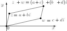
The addition of complex numbers has a geometric description. The diagram shows plots of the complex numbers z = a + bi and ![]() and their sum
and their sum ![]() . These points, together with the origin, form the vertices of a parallelogram, so we can find the sum
. These points, together with the origin, form the vertices of a parallelogram, so we can find the sum ![]() geometrically by completing the parallelogram. This method is the Parallelogram Law of Complex Addition and is a special case of vector addition, as students of linear algebra will recognize.
geometrically by completing the parallelogram. This method is the Parallelogram Law of Complex Addition and is a special case of vector addition, as students of linear algebra will recognize.
The geometric description of complex multiplication requires that complex num-bers be represented in polar coordinates. The circle with its center at the origin and radius 1 shown in the diagram below is called the unit circle. An angle θ measured counterclockwise from the real axis is said to be in standard po-sition. The angle θ determines a unique point P on this circle. The radian measure of θ is defined to be the length of the arc from 1 to P. Hence, the radian measure of a right angle is π/2 radians and that of a full circle is 2π radians. We define the cosine and sine of θ (written cos θ and sin θ) to be the x and y coordinates of P. Hence, P is the point (cos θ, sin θ) = cos θ + i sin θ in the complex plane. These complex numbers cos θ + i sin θ on the unit circle are denoted eiθ = cos θ + i sin θ.

![]()
A complete discussion of why we use this notation lies outside the scope of this book.139
The fact that eiθ is actually an exponential function of θ is confirmed by verifying that the law of exponents holds, that is,
![]()
This law is analogous to the exponent rule eaeb = ea+b for real exponents a and b, and it is an immediate consequence of the identities for sin (θ + ![]() ) and cos (θ +
) and cos (θ + ![]() ):
):

We can now describe complex multiplication geometrically. We let z = a + bi be any complex number. The distance r from z to 0 is the modulus r = |z|. If z ≠ 0, it determines an angle θ, as shown in the diagram, called an argument of z. This angle is not unique (θ + 2πk would do as well for any k = 0, ± 1, ± 2, . . .,) but, as the diagram clearly shows,

always hold. Hence, in any case
![]()
This expression is the polar form of the complex number z. The geometric description of complex multiplication follows from the law of exponents.
Theorem 4. Multiplication Rule. If z = reiθ and ![]() are two complex numbers in polar form, then
are two complex numbers in polar form, then
![]()
In other words, to multiply two complex numbers, simply multiply the absolute values and add the arguments. This method simplifies calculations and is valid for any arguments θ and ![]() .
.
Example 4. Multiply ![]() by first converting the factors to polar form.
by first converting the factors to polar form.
Solution. The polar forms (see the diagram) are

Hence, the multiplication rule gives

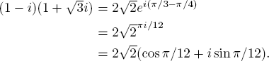
Of course, direct multiplication gives ![]() so equating real and imaginary parts gives the (somewhat unexpected) formulas
so equating real and imaginary parts gives the (somewhat unexpected) formulas
![]()
If z = reiθ is given in polar form, z2 = r2e2iθ by the multiplication rule. Hence, z3 = (reiθ)(r2e2iθ) = r3e3iθ. In general, we have Theorem 5 for any n ≥ 1 (we leave the proof for n ≤ 0 as Exercise 15(b)). The name honors Abraham DeMoivre (1667-1754).
Theorem 5. DeMoivre's Theorem. If θ is any angle and r > 0, then (reiθ)n = rneinθ for all integers n.
Example 5. Verify that ![]()
The polar form is ![]() Hence DeMoivre's theorem gives
Hence DeMoivre's theorem gives
![]()
If n ≥ 1, a complex number u is called an nth root of unity if un = 1. DeMoivre's theorem gives a way to find all possibilities (there are n). If we write u = reiθ in polar form and use DeMoivre's theorem, the condition un = 1 becomes
![]()
Comparing absolute values gives rn = 1, so r = 1 (because r is real and positive). However, the arguments may differ by integral multiples of 2π, so all we can conclude is that nθ = 2kπ, where k is an integer; that is,
![]()
These arguments give distinct values of u on the unit circle for k = 0, 1, 2, . . ., n − 1, as shown in the di-agram. But every choice of k yields a value of θ differing from one of these by a multiple of 2π, so they give all the possible roots. This proves Theorem 6.

Theorem 6. The nth roots of unity are ![]() for k = 0, 1, 2, . . ., n − 1.
for k = 0, 1, 2, . . ., n − 1.
We find these roots geometrically as the distinct points on the unit circle, starting at 1, that cut the circle into n equal sectors. Note that if n = 2, the roots are 1 and −1, whereas the four 4th roots of unity are 1, i, − 1, and −i. In general, if we write ![]() then the nth then
then the nth then ![]() for each k ≥ 1, so the nth roots of unity are just the powers of
for each k ≥ 1, so the nth roots of unity are just the powers of ![]()
![]()
For this reason, ![]() is called a primitive nth root of unity. It follows easily (Exercise 16) that
is called a primitive nth root of unity. It follows easily (Exercise 16) that ![]() that is, the sum of the nth roots of unity is zero.
that is, the sum of the nth roots of unity is zero.
1. Solve each equation for the real number x.
(a) x − 4i = (2 − i)2
(b) (2 + xi)(3 − 2i) = 12 + 5i
(c) (2 + xi)2 = 4
(d) (2 + xi)(2 − xi) = 5
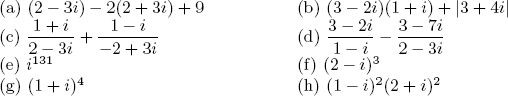
2. Convert each expression to the form a + bi.
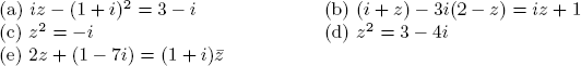
3. In each case, find the complex number z.
4. Let rez and imz denote the real and imaginary parts of z. Show that

5. In each case, describe the graph of the equation, where z denotes a complex number

6. Verify ![]() directly for z = a + bi and
directly for z = a + bi and ![]()
7. Prove that ![]() for all complex numbers
for all complex numbers ![]() and z.
and z.
8. Show that (1 + i)n + (1 − i)n is real for all integers n ≥ 1.
9.
(a) Complex Distance Formula. Show that ![]() is the distance between the complex numbers z and
is the distance between the complex numbers z and ![]()
(b) Triangle Inequality. Show that ![]() for all complex numbers z and
for all complex numbers z and ![]() [Hint: Consider the triangle with vertices
[Hint: Consider the triangle with vertices ![]() and
and ![]() ]
]
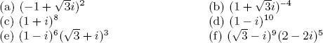
10. Write each expression in polar form.
![]()
11. Write each expression in the form a + bi.
![]()
12. Write each expression in the form a + bi.
13. Use DeMoivre's theorem to show that
![]()
14. Find all complex numbers such that
![]()
15. Let z = reiθ in polar form.
![]()
16. Show that the sum of the nth roots of unity is 0.
![]()
17.
(a) Suppose that z1, z2, z3, z4, and z5 are equally spaced around the unit circle. Show that z1 + z2 + z3 + z4 + z5 = 0. [Hint: (1 − z)(1 + z + z2 + z3 + z4) = 1 − z5 for any complex number z.]
(b) Repeat (a) for any n ≥ 2 points placed equally around the unit circle.
18. If z = a + bi, show that ![]() [Hint: (|a| − |b|)2 ≥ 0.]
[Hint: (|a| − |b|)2 ≥ 0.]
19. Let f(x) = a0 + a1x + a2x2 + ![]() + anxn be a polynomial with real coefficients ai. If z is a complex root of f(x), that is, f(z) = 0, show that
+ anxn be a polynomial with real coefficients ai. If z is a complex root of f(x), that is, f(z) = 0, show that ![]() is also a root.
is also a root.
20. If f(x) is a polynomial with complex coefficients, let ![]() be the polynomial obtained from f(x) by taking the conjugate of every coefficient. Show that
be the polynomial obtained from f(x) by taking the conjugate of every coefficient. Show that ![]() is a polynomial with real coefficients.
is a polynomial with real coefficients.
21. Let z ≠ 0 be a complex number. If t is real, describe tz geometrically if
(a) t > 0
(b) t < 0
22. If z and ![]() are nonzero complex numbers, show that
are nonzero complex numbers, show that ![]() if and only if one is a positive real multiple of the other. [Hint: Consider the parallelogram with vertices
if and only if one is a positive real multiple of the other. [Hint: Consider the parallelogram with vertices ![]() and
and ![]() Use Exercise 21 and the fact that, if t is real, |1 + t| = 1 + |t| is impossible if t < 0.]
Use Exercise 21 and the fact that, if t is real, |1 + t| = 1 + |t| is impossible if t < 0.]
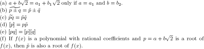
23. If a and b are rational numbers, let p and q denote numbers of the form ![]() If
If ![]() define
define ![]() and [p] = a2 − 2b2. Show that each of the following expressions holds.
and [p] = a2 − 2b2. Show that each of the following expressions holds.
Matrix algebra will be familiar to most readers as it is standard fare in beginning linear algebra courses. The new ingredient here is that the matrices we consider will have entries drawn from an arbitrary commutative ring R, rather than from the real numbers ![]() A ring is an algebraic system in which there are two operations, addition and multiplication, for which the usual laws of arithmetic are valid (see Section 3.1). A ring R is called commutative if ab = ba for all a, b
A ring is an algebraic system in which there are two operations, addition and multiplication, for which the usual laws of arithmetic are valid (see Section 3.1). A ring R is called commutative if ab = ba for all a, b ![]() R. Examples include the familiar number systems
R. Examples include the familiar number systems ![]() and
and ![]() It is worth noting that the set
It is worth noting that the set ![]() of all 2 × 2 matrices over
of all 2 × 2 matrices over ![]() is a ring that is not commutative.
is a ring that is not commutative.
In this appendix, the standard results from linear algebra about matrices, adjugates, inverses, determinants, and so on, will be stated, with suitable minor modifications, over an arbitrary commutative ring R. We omit most proofs. When ![]() many proofs from linear algebra remain valid, but this is often not the case. It is important to note that it is essential that R is commutative in many arguments, especially when dealing with inverses and determinants. Hence,
many proofs from linear algebra remain valid, but this is often not the case. It is important to note that it is essential that R is commutative in many arguments, especially when dealing with inverses and determinants. Hence,
R denotes a commutative ring throughout Appendix B.
Matrix Algebra
A rectangular array of elements of R is called a matrix and the elements themselves are called the entries of the matrix. Thus,
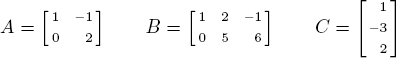
are matrices over ![]() The shape of a matrix depends on the number of rows and columns, and an m × n matrix is one with m rows and n columns. Two matrices are the same size if they have the same number of rows and the same number of columns. Thus, the preceding matrices A, B, and C are of size 2 × 2, 2 × 3, and 3 × 1, respectively. An n × n matrix is called a square matrix.
The shape of a matrix depends on the number of rows and columns, and an m × n matrix is one with m rows and n columns. Two matrices are the same size if they have the same number of rows and the same number of columns. Thus, the preceding matrices A, B, and C are of size 2 × 2, 2 × 3, and 3 × 1, respectively. An n × n matrix is called a square matrix.
The rows and columns of a matrix are numbered from the top down and from left to right, respectively. Then the entry in row i and column j of a matrix A is called the (i, j)-entry of A. If the (i, j)-entry is denoted aij, then A has the form

which usually is abbreviated as A = [aij]. Two m × n matrices A = [aij] and B = [bij] are equal (written A = B) if they have the same size and corresponding entries are equal, that is
![]()
The set of all m × n matrices with entries from R is denoted Mmn(R). For A and B in Mmn(R), we obtain their sum A + B by adding corresponding entries. If A = [aij] and B = [bij], this is
![]()
This addition enjoys many of the properties of numerical addition. For example, if A, B, and C are in Mmn(R), then
A + B = B + A and A + (B + C) = (A + B) + C.
The matrix in Mmn(R) each of whose entries is zero is called the zero matrix of size m × n and is denoted 0 (or 0mn if the size must be emphasized). Clearly,
A + 0 = A, for all A in Mmn(R).
So 0 plays the role in Mmn(R) that the number zero plays in ![]() We obtain the negative −A of a matrix A in Mmn(R) by negating every entry of A. Hence,
We obtain the negative −A of a matrix A in Mmn(R) by negating every entry of A. Hence,
A + (− A) = 0, for all A in Mmn(R).
Finally we define subtraction by A − B = A + (− B). If A = [aij] and B = [bij],
−A = [− aij] and A − B = [aij − bij].
With these definitions, the additive arithmetic in Mmn(R) is entirely analogous to numerical arithmetic.
We also use the following notation: If A is a matrix and r ![]() R, the matrix rA is obtained by multiplying every entry of A by r. More formally
R, the matrix rA is obtained by multiplying every entry of A by r. More formally
If A = [aij] then rA = [raij].
This is called scalar multiplication and one verifies that it enjoys the following useful properties for all scalars r, s and matrices A, B:
1. r(A + B) = rA + rB
2. (r + s)A = rA + sA
3. r(sA) = (rs)A
4. 1A = A
Example 1. Given ![]() and
and ![]() in
in ![]() we have
we have
![]()
Example 2. If ![]() and
and ![]() in M23(R), find X in M23(R) such that X + A = B.
in M23(R), find X in M23(R) such that X + A = B.
Solution. We proceed as in numerical arithmetic and subtract A from both sides:
![]()
Multiplication of matrices is less natural than addition. To describe it, we define the dot product of a row matrix and a column matrix as follows:
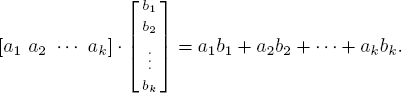
Now let A be an m × k matrix and B be a k × n matrix, chosen so that the rows of A and the columns of B have the same number k of entries. Then the product AB is defined to be the m × n matrix whose
(i, j)-entry is the dot product of row i of A and column j of B.
Thus to compute the (i, j)-entry, go across the ith row of A and down the jth column of B and form the dot product. Note: If A is m × k and B is k′ × n, then
AB is defined only if k = k′, and then the product AB is m × n.
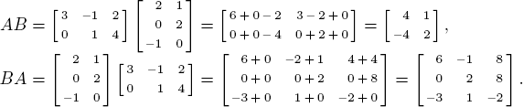
Example 3. For ![]() and
and ![]() compute AB and BA.
compute AB and BA.
Solution. We write out the dot products explicitly.
Example 4. If ![]() and
and ![]() compute A2, AB, and BA.
compute A2, AB, and BA.
Solution. ![]()
so A2 = 0 can occur even when A ≠ 0. Next
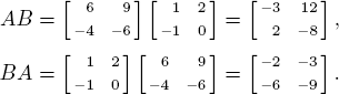
Hence AB ≠ BA is possible even though they are both the same size.
Example 4 shows that two familiar properties of numerical algebra fail for matrices. Hence, it is surprising to learn that the following property does hold.
Theorem 1. Let A, B, and C be of sizes m × p, p × q, and q × n, respectively. Then (AB)C = A(BC).
Proof. Write A = [aij], B = [bij], and C = [cij]. Then AB = [xij] where we have ![]() and (AB)C = [yij] where
and (AB)C = [yij] where ![]() Hence,
Hence,
![]()
This last expression is the (i, j)-entry of A(BC), and the theorem follows. Note that we needed the associativity of R to get aik(bktctj) = aikbktctj = (aikbkt)ctj.
We express this result by saying that matrix multiplication is associative when the matrix sizes are such that the products involved are all defined.
The number 1 plays a neutral role in numerical multiplication in the sense that 1a = a and a 1 = a for every number a. The analogous role in matrix algebra is played by the identity matrices In. For each n ≥ 1, the matrix In is defined to be the n × n matrix with 1s along the main diagonal (upper left to lower right), and 0s elsewhere. Thus,
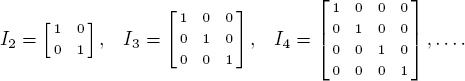
We use I without a subscript for the identity matrix when there is no need to emphasize the size. The reader can verify that the relations
![]()
hold whenever the matrix products are defined.
Note that rA = (rI)A for all r ![]() R and all matrices A. Moreover, since R is commutative we have (when the matrix multiplications are defined)
R and all matrices A. Moreover, since R is commutative we have (when the matrix multiplications are defined)
r(AB) = (rA)B = A(rB), for all r ![]() R.
R.
Square Matrices and Inverses
We are interested primarily in square matrices. For convenience, we use the notation
Mn(R) = Mnn(R), for any n ≥ 2.
If A and B lie in Mn(R) then A + B and AB are both in Mn(R). Theorem 2 collects several properties of Mn(R) for reference later.
Theorem 2. Let A, B, and C be matrices in Mn(R). Then
1. A + B = B + A
2. (A + B) + C = A + (B + C)
3. A + 0 = A
4. A + (− A) = 0
5. (AB)C = A(BC)
6. AI = A = IA
7. A(B + C) = AB + AC and (B + C)A = BA + CA
Proof. The only property not discussed previously is (7), and we leave the verification as Exercise 12.
The reader may have noted that Theorem 2 shows that Mn(R) is a ring (noncommutative if n ≥ 2). It is also noteworthy that Theorem 2 holds even if the ring R is not commutative.
If A is a square matrix, a matrix B is called an inverse of A if
![]()
If it exists, this matrix B is uniquely determined by A. For if AC = I also holds, then AC = AB (both equal to I) so left multiplication by B gives C = B. A square matrix A is called invertible if it has an inverse, and in this case the (unique) inverse is denoted A−1. Note that 0 has no inverse; in fact if AB = 0 for some B ≠ 0 then A has no inverse.
Write Rn for the set of n × 1 column matrices with entries from R. If ![]() it is known that A is invertible if and only if the system AX = B of linear equations has a solution X for any
it is known that A is invertible if and only if the system AX = B of linear equations has a solution X for any ![]() This holds in general because AB = I in Mn(R) implies BA = I (Exercise 13). On the other hand, if
This holds in general because AB = I in Mn(R) implies BA = I (Exercise 13). On the other hand, if ![]() it is known that A is invertible if and only if the homogeneous linear system AX = 0 has only the trivial solution X = 0. But this condition fails for
it is known that A is invertible if and only if the homogeneous linear system AX = 0 has only the trivial solution X = 0. But this condition fails for ![]() (consider A = 2I). Hence if A is a square matrix, we need other ways to determine when A−1 exists.
(consider A = 2I). Hence if A is a square matrix, we need other ways to determine when A−1 exists.
Again, it is well known that ![]() is invertible if and only if det A ≠ 0. If R is any commutative ring it turns out that the determinant of A
is invertible if and only if det A ≠ 0. If R is any commutative ring it turns out that the determinant of A ![]() Mn(R) can be defined in such a way that A is invertible if and only if det A is a unit in R (u
Mn(R) can be defined in such a way that A is invertible if and only if det A is a unit in R (u ![]() R is a unit if uv = 1 = vu for some
R is a unit if uv = 1 = vu for some ![]() The idea is to define det A inductively. If n = 1 and A = [a], this holds if we define
The idea is to define det A inductively. If n = 1 and A = [a], this holds if we define
det [a] = a.
If n ≥ 2, assume inductively that det A has been defined for all (n − 1) × (n − 1) matrices over R. If A is n × n write Aij for the (n − 1) × (n − 1) matrix obtained from A by deleting row i and column j. Then, given 1 ≤ i, j ≤ n we define the (i, j) -cofactor of A by
cij(A) = (− 1)i+j det Aij.
With this, we define det A as follows:
(*) det A = a11 c11(A) + a21 c21(A) + ![]() + an 1 cn 1(A).
+ an 1 cn 1(A).
Then one shows that the following properties of determinants hold for rows:
1. If B is formed by multiplying a row of A by u ![]() R, then det B = u det A.
R, then det B = u det A.
2. If A contains a row of zeros then det A = 0.
3. If two rows of A are interchanged then det A changes sign.
4. If a multiple of a row of A is added to a different row, then det A is unchanged.
5. If two rows of A are identical then det A = 0.
With this one can prove a result first given (for ![]() in 1772 by Pierre Simon de Laplace.
in 1772 by Pierre Simon de Laplace.
Theorem 3. Cofactor Expansion Theorem. If A = [aij] is an n × n matrix over a commutative ring R, then
1. ![]() , for each j = 1, 2, . . ., n,
, for each j = 1, 2, . . ., n,
2. ![]() , for each i = 1, 2, . . ., n.
, for each i = 1, 2, . . ., n.
Furthermore, (a)–(e) above hold for rows and for columns.
We omit the details.140 The expressions in (1) and (2) of Theorem 3 are called the cofactor expansions along column j and row i, respectively. In words, to find the cofactor expansion of det A along a row or column, multiply the entries of the row (column) by the corresponding cofactors, and add the results.
The cofactor expansion theorem has many important consequences, and the following result is necessary to describe them. Given an n × n matrix A = [aij], the transpose AT of A is defined by
AT = [bij], where bij = aji for all i and j.
This is an n × n matrix obtained from A by interchanging elements symmetric about the main diagonal. For example, if ![]() then
then ![]() The familiar elementary properties of the transpose hold
The familiar elementary properties of the transpose hold
1. (A + B)T = AT + BT
2. (rA)T = rAT
3. (AB)T = BTAT)
when the matrix operations are defined (even for nonsquare matrices). We omit the proof of the following theorem.
Theorem 4. Transpose Theorem. If A is a square matrix then det AT = det A.
Surprisingly, the determinant function preserves matrix multiplication. Again we omit the proof.
Theorem 5. Multiplication Theorem. If A and B are n × n matrices then
det (AB) = det A det B.
Given an n × n matrix A = [aij] over a commutative ring R, we define the adjugate of A (also called the classical adjoint of A) as follows:
adj A = [cij(A)]T.
This is also n × n and the cofactor expansion theorem (with some ingenuity) gives
Theorem 6. Adjugate Theorem. If A is n × n and d = det A, then
A (adj A) = dIn = (adj A) A.
Again we omit the details.
If it happens that d = det A is a unit in R, then (as R is commutative) the adjugate theorem gives
A[d−1 adj (A)] = In = [d−1 adj (A)]A,
from which A is invertible and A−1 = d−1 adj (A). This proves part of
Theorem 7. Invertibility Theorem. If A is n × n then A is invertible if and only if det A is a unit in R. In this case det (A−1) = (det A)−1.
The rest of the proof follows from Theorem 5 (Exercise 14).
The case of 2 × 2 matrices is simple and so arises frequently in examples. The relevant facts are displayed next.
Example 5. If n = 2 and ![]() then we have adj
then we have adj ![]() and det A = ad − bc. Hence, if ad − bc is a unit in R then
and det A = ad − bc. Hence, if ad − bc is a unit in R then ![]() is a convenient formula for the inverse of A.
is a convenient formula for the inverse of A.
These results are enough to do most of the calculations in this book. A good reference source for this material (and much more) is the book by McDonald, B.R. Linear Algebra over Commutative Rings, Marcel Dekker Inc., New York, 1984.
Multilinear Approach
An n × n matrix A can be thought of as a row of columns in Rn, and it is instructive to view matrices that way. Hence, we write A = [A1, . . ., Ak, . . ., An], where Ak denotes column k of A. The determinant function det: Mn(R) → R has two basic properties from this point of view.
First, det is a multilinear function of the columns of a matrix, that is, it is a linear function of column k for each k (when we fix all other columns of A). More precisely, if we define
![]()
the requirement is that, for each k,
δk(rX + sY) = rδk(X) + sδk(Y) for all r, s ![]() R and X, Y
R and X, Y ![]() Rn.
Rn.
Second, det is an alternating function of the columns of a matrix; that is if two distinct columns of A are interchanged to form B, then det B = − det A.
Before proceeding, write Xn = {1, 2, . . ., n} and recall the symmetric group Sn (see Section 1.4) of all permutations of Xn, that is all bijections σ: Xn → Xn. Each such σ is a product of transpositions, that is permutations that interchange two members of Xn. And σ is called even or odd according as it can be expressed as a product of an even, respectively odd, number of transpositions (the parity theorem ensures that this is well defined). The sign of σ is defined to be 1 or −1 according as σ is even or odd, and is written (− 1)σ.
Hence, the fact that det is alternating means that if B is obtained from A by a series of column transpositions, then det B = (− 1)σ det A where σ is the corresponding column permutation. With this it can be shown that d = det is the only multilinear, alternating function d: Mn(R) → R that satisfies d(I) = 1. Moreover, if we write σ(k) = σk when σ ![]() Sn and k
Sn and k ![]() Xn, the following characterization of det A can be proved.
Xn, the following characterization of det A can be proved.
Theorem 8. If A = [aij] is n × n then ![]() where the sum ranges over all n! elements σ of Sn.
where the sum ranges over all n! elements σ of Sn.
Theorem 8 leads to other important properties of the determinant, and is often taken as the definition.
Throughout these exercises, R is assumed to be a commutative ring.
1. If A is square, AB = 0, and B ≠ 0, show that A cannot be invertible.
2.
(a) If B = [B1, . . ., Bk, . . ., Bn] where Bk is column k of B, show that AB = [AB1, . . ., ABk, . . ., ABn].
(b) If AX = 0 for every X ![]() Rn, show that A = 0.
Rn, show that A = 0.
3. If ![]() and
and ![]() show that AB = I2 but BA ≠ I3.
show that AB = I2 but BA ≠ I3.
4. Show that ![]() is invertible in M2(R) if and only if a and c are both units. In this case find A−1.
is invertible in M2(R) if and only if a and c are both units. In this case find A−1.
5. Find invertible 2 × 2 matrices A and B such that A + B is not invertible.
6. Find a matrix X such that AX = B if ![]() and
and ![]()
7. If A and B are n × n, show that (A − B)(A + B) = A2 − B2 if and only if AB = BA.
8. If A2 = 0, show that I + A is invertible and find (I + A)−1 in terms of A.
9. If ![]() show that A3 = I and use this result to find A−1 in terms of A.
show that A3 = I and use this result to find A−1 in terms of A.
10. Show that ![]() satisfies A2 − 3A − 10I = 0 and use this result to find A−1 in terms of A.
satisfies A2 − 3A − 10I = 0 and use this result to find A−1 in terms of A.
11. Let A and B denote n × n matrices.
(a) If A and B are invertible, show that A−1 and AB also are invertible, and find formulas for the inverses.
(b) If A, B and A + B are invertible, show that A−1 + B−1 is also invertible find a formula for the inverse.
(c) If I + BA is invertible show that I + AB is invertible and find a formula for (I + AB)−1. [Hint: A(I + BA) = (I + AB)A.]
12. Prove (7) of Theorem 2. (These expressions are called the distributive laws.)
13.
(a) If A, B ![]() Mn(R), show that AB = I implies that BA = I.
Mn(R), show that AB = I implies that BA = I.
(b) Show that A is invertible if and only if AX = B has a solution for every B ![]() Rn. [Hint: Write I = [E1, . . ., Ek, . . ., En], use (a) Exercise 2(a).]
Rn. [Hint: Write I = [E1, . . ., Ek, . . ., En], use (a) Exercise 2(a).]
14. Prove Theorem 7 using Theorems 5 and 6.
15. Let Eij denote the matrix in Mn(R) with (i, j) -entry 1 and all other entries 0.
(a) Show that EikEmj = δkmEij where δkm = 0 or 1 according as k = m or k ≠ m.
(b) Show that E11 + E22 + ![]() + Enn = I.
+ Enn = I.
(c) Show that if A = [aij] ![]() Mn(R) then A = Σi,jaijEij.
Mn(R) then A = Σi,jaijEij.
Here the Eij are called matrix units in Mn(R), and δkm is called the Kronecker delta.
The independent sets in a vector space are undeniably important, but the largest independent sets are the most important of all: they are the bases of the space. This theme that the “ largest” objects of a given type are the most interesting is universal in mathematics, certainly in algebra. Zorn's lemma is a set-theoretical principle that shows that maximal objects of various types exist and has become indispensable in many parts of mathematics. Clarifying what “ maximal” means is best formulated using the concept of a partial ordering.
A partial order on a nonempty set P is a relation141 ≤ on P that satisfies the following conditions (where x, y, and z denote elements of P):

A set P with a partial ordering is called a partially ordered set (poset for short). We say that (P, ≤) is a poset to assert that ≤ is a partial ordering on the set P. Posets occur everywhere in mathematics; here are a few examples.
The following are easily verified to be partial orders:
Inclusion ⊆ on any nonempty collection of sets.
Divisibility ![]() on any nonempty set of positive integers.
on any nonempty set of positive integers.
The usual ordering ≤ on the set ![]() of real numbers.
of real numbers.
Nonempty subsets of a poset are again posets with the same partial order.
Other examples will occur later.
If ≤ is a partial order on a set P, we write x < y to mean x ≤ y and x ≠ y. An element m ![]() P is called maximal in P if there is no element x of P such that m < x, or equivalently,
P is called maximal in P if there is no element x of P such that m < x, or equivalently,
![]()
For example, if U is any nonempty set, let ![]() denote the set of proper subsets X ⊂ U. Then the maximal members of
denote the set of proper subsets X ⊂ U. Then the maximal members of ![]() (under inclusion) are the sets U {a} omitting one element a
(under inclusion) are the sets U {a} omitting one element a ![]() U. Here is a more algebraic example.
U. Here is a more algebraic example.
Example 1. If R is a ring, the maximal ideals of R (Section 3.3) are defined to be the maximal members of the poset ![]() is an ideal of R} partially ordered by inclusion. If R is commutative, corollary 1 of Theorem 6 §3.3 shows that an ideal A is maximal if and only if the factor ring R/A is a field.
is an ideal of R} partially ordered by inclusion. If R is commutative, corollary 1 of Theorem 6 §3.3 shows that an ideal A is maximal if and only if the factor ring R/A is a field.
Zorn's lemma gives a condition that guarantees that maximal elements exist in certain posets. To state it, we need some terminology. Let (P, ≤) be a poset. If X ⊆ P is a nonempty subset, an element u ![]() P is called an upper bound for X if x ≤ u for every x
P is called an upper bound for X if x ≤ u for every x ![]() X. Note that u need not be an element of X. For example, in the poset
X. Note that u need not be an element of X. For example, in the poset ![]() the interval
the interval ![]() has no maximal member, but any number u ≥ 1 is an upper bound on X.
has no maximal member, but any number u ≥ 1 is an upper bound on X.
If we are looking for maximal elements in a poset P, choose x1 ![]() P. If x1 is maximal, we are done. Otherwise, x1 < x2 for some x2
P. If x1 is maximal, we are done. Otherwise, x1 < x2 for some x2 ![]() P. If x2 is maximal, we are finished; otherwise x1 < x2 < x3 for some x3
P. If x2 is maximal, we are finished; otherwise x1 < x2 < x3 for some x3 ![]() P. Hence, either we find a maximal element at some stage, or we create elements x1, x2, x3, . . . in P such that x1< x2 < x3 <
P. Hence, either we find a maximal element at some stage, or we create elements x1, x2, x3, . . . in P such that x1< x2 < x3 < ![]() is a strictly increasing sequence. So it is plausible that guaranteeing the existence of maximal elements in P will require some restriction on such ascending sequences from P. In 1935, Max Zorn found a condition on P that does this and is reasonably easy to verify in specific situations.
is a strictly increasing sequence. So it is plausible that guaranteeing the existence of maximal elements in P will require some restriction on such ascending sequences from P. In 1935, Max Zorn found a condition on P that does this and is reasonably easy to verify in specific situations.
Two elements x and y in a poset P are called comparable if either x ≤ y or y ≤ x, and the poset P is called a chain if any two elements are comparable. Thus, ![]() is a chain with respect to the usual partial ordering. A partially ordered set P is said to be inductive if every chain in P has an upper bound in P.
is a chain with respect to the usual partial ordering. A partially ordered set P is said to be inductive if every chain in P has an upper bound in P.
Theorem. Zorn's Lemma. Every inductive partially ordered set has a maximal element.
Note that to show that a poset is inductive, it is not enough to check that all countable142 chains x1< x2 < x3 < ![]() have upper bounds in P. For example, consider the set
have upper bounds in P. For example, consider the set ![]() of all countable subsets of
of all countable subsets of ![]() partially ordered by inclusion. Then every countable chain in
partially ordered by inclusion. Then every countable chain in ![]() has an upper bound in
has an upper bound in ![]() , namely, its union (since unions of countable sets are again countable). But
, namely, its union (since unions of countable sets are again countable). But ![]() has no maximal member because such a maximal set would have to be
has no maximal member because such a maximal set would have to be ![]() itself, and
itself, and ![]() is not a countable set.
is not a countable set.
Zorn's lemma has a wide variety of applications throughout mathematics; we give three examples from algebra. We begin with vector spaces. In Section 6.1, we proved that every finite dimensional vector space has a basis, but the proof that this holds in the infinite dimensional case requires Zorn's lemma. If V is a vector space over a field F, let X be a nonempty (possibly infinite) subset of V. Then X is called independent if every finite subset of X is independent (in the sense of Section 6.1), and X is said to span V if every element of V is a linear combination of (a finite number of) elements of X, Finally, X is called a basis of V if it is independent and spans V.
Example 2. If F is a field, show that every nonzero vector space V has a basis.
Solution. The idea is to show that any maximal independent set is a basis. Let ![]() denote the set of all independent sets in V and partially order
denote the set of all independent sets in V and partially order ![]() by inclusion. We begin by using Zorn's lemma to show that
by inclusion. We begin by using Zorn's lemma to show that ![]() has maximal members. First,
has maximal members. First, ![]() is not empty since
is not empty since ![]() is in
is in ![]() for all
for all ![]() in V. Suppose that
in V. Suppose that ![]() is a chain in
is a chain in ![]() if
if ![]() , we claim that X is independent. To see this, let {x1, x2, . . ., xn} be a finite subset of X. Then each xk is in some Xi, so, since Xi form a chain, {x1, x2,
, we claim that X is independent. To see this, let {x1, x2, . . ., xn} be a finite subset of X. Then each xk is in some Xi, so, since Xi form a chain, {x1, x2, ![]() , xn} ⊆ Xm for some m. Hence, {x1, x2, . . ., xn} is independent (since Xm is in
, xn} ⊆ Xm for some m. Hence, {x1, x2, . . ., xn} is independent (since Xm is in ![]() ), as required. This shows that X is in
), as required. This shows that X is in ![]() and so is an upper bound for
and so is an upper bound for ![]() in
in ![]()
Now Zorn's lemma shows that ![]() has a maximal member B, and we claim that B is a basis of V. Since it is independent (being in
has a maximal member B, and we claim that B is a basis of V. Since it is independent (being in ![]() ), it remains to prove that span(B) = V, where span(B) consists of all linear combinations of vectors in B. Assume on the contrary that
), it remains to prove that span(B) = V, where span(B) consists of all linear combinations of vectors in B. Assume on the contrary that ![]() we show that
we show that ![]() is independent, contradicting the maximality of B.
is independent, contradicting the maximality of B.
So let X be a finite subset of ![]() we must show that X is independent. If X ⊆ B, this follows because
we must show that X is independent. If X ⊆ B, this follows because ![]() If
If ![]() , then
, then ![]() , so write
, so write ![]() , xi
, xi ![]() B. Let
B. Let ![]() ai
ai ![]() F. Then a0 = 0 because otherwise
F. Then a0 = 0 because otherwise ![]() , contrary to our choice (since
, contrary to our choice (since ![]() exists in the field F). Hence, a1x1 + a2x2 +
exists in the field F). Hence, a1x1 + a2x2 + ![]() + anxn = 0, so ai = 0 for i ≥ 1, as required.
+ anxn = 0, so ai = 0 for i ≥ 1, as required.
It is worth noting that Example 2 is true for any division ring in place of F. In fact, most of the theory of vector spaces goes through for division rings.
The next two examples of Zorn's lemma come from ring theory. An additive subgroup L of a ring R is called a left ideal if Ra ⊆ L for all a ![]() L, where Ra = {ra
L, where Ra = {ra ![]() r
r ![]() R}. Right ideals are defined similarly, and the ideals of R (see Section 3.3) are just the left and right ideals. A maximal left ideal M is defined to be a maximal member of {L ≠ R
R}. Right ideals are defined similarly, and the ideals of R (see Section 3.3) are just the left and right ideals. A maximal left ideal M is defined to be a maximal member of {L ≠ R ![]() L is a left ideal}, partially ordered by inclusion.
L is a left ideal}, partially ordered by inclusion.
Example 3. If L ≠ R is any left ideal, then L is contained in a maximal left ideal.
Solution. Let ![]() is a left ideal and L ⊆ X ≠ R}, partially ordered by inclusion. Then
is a left ideal and L ⊆ X ≠ R}, partially ordered by inclusion. Then ![]() is not empty (
is not empty (![]() so it suffices to show that
so it suffices to show that ![]() contains a maximal element. By Zorn's lemma, it is enough to show that
contains a maximal element. By Zorn's lemma, it is enough to show that ![]() is inductive. Hence, let {Xi
is inductive. Hence, let {Xi ![]() i
i ![]() I} be a chain from
I} be a chain from ![]() ; we show that
; we show that ![]() is an upper bound for {Xi}. Clearly, X is a left ideal containing L, and we claim that X ≠ R. For if X = R, then 1
is an upper bound for {Xi}. Clearly, X is a left ideal containing L, and we claim that X ≠ R. For if X = R, then 1 ![]() X, say 1
X, say 1 ![]() Xk for some k
Xk for some k ![]() I. Since Xk is a left ideal, it follows that R = R 1 ⊆ Xk ⊆ R, so Xk = R, contrary to the fact that
I. Since Xk is a left ideal, it follows that R = R 1 ⊆ Xk ⊆ R, so Xk = R, contrary to the fact that ![]() So X is an upper bound in
So X is an upper bound in ![]() on the chain {Xi}, as required.
on the chain {Xi}, as required.
As our last example of the use of Zorn's lemma, we prove a theorem that is of central importance in the theory of commutative rings. Let R be a commutative ring. An ideal P of R is called a prime ideal of R if R/P is an integral domain, or equivalently, if rs ![]() P, where r, s
P, where r, s ![]() R, then either r
R, then either r ![]() P or s
P or s ![]() P (see Theorem 3 §3.3). Every commutative ring has at least one prime ideal by Example 3 (since maximal ideals are prime in any commutative ring).
P (see Theorem 3 §3.3). Every commutative ring has at least one prime ideal by Example 3 (since maximal ideals are prime in any commutative ring).
An element a ![]() R is said to be nilpotent if an = 0 for some n ≥ 1, and the set nil(R) of all nilpotents in a commutative ring R is called the nil radical of R. It is easy to verify that nil(R) ⊆ P for every prime ideal P, and hence that nil(R) ⊆ ∩ {P
R is said to be nilpotent if an = 0 for some n ≥ 1, and the set nil(R) of all nilpotents in a commutative ring R is called the nil radical of R. It is easy to verify that nil(R) ⊆ P for every prime ideal P, and hence that nil(R) ⊆ ∩ {P ![]() P is a prime ideal of R}. The following example uses Zorn's lemma to show that this is in fact equality.
P is a prime ideal of R}. The following example uses Zorn's lemma to show that this is in fact equality.
Example 4. If R is a commutative ring, nil(R) = ∩ {P ![]() P is a prime ideal of R}.
P is a prime ideal of R}.
Solution. Let a ![]() P for every prime ideal P; by the above remarks, we must show that a is nilpotent. So we assume that a is not nilpotent and show (using Zorn's Lemma) that a ∉ P for some prime ideal P. To this end, let
P for every prime ideal P; by the above remarks, we must show that a is nilpotent. So we assume that a is not nilpotent and show (using Zorn's Lemma) that a ∉ P for some prime ideal P. To this end, let
![]() is an ideal of R and an ∉ A for every n ≥ 1}.
is an ideal of R and an ∉ A for every n ≥ 1}.
Then ![]() is not empty as
is not empty as ![]() since a is not nilpotent. Suppose {Ai
since a is not nilpotent. Suppose {Ai ![]() i
i ![]() I} is a chain from
I} is a chain from ![]() , and let A =
, and let A = ![]() i
i![]() IAi. Then A is an ideal and if an
IAi. Then A is an ideal and if an ![]() A, then an
A, then an ![]() Ak for some k, contradicting the fact that
Ak for some k, contradicting the fact that ![]() Hence, an ∉ A for each n, and so
Hence, an ∉ A for each n, and so ![]() This shows that
This shows that ![]() is inductive, so, by Zorn's lemma, let
is inductive, so, by Zorn's lemma, let ![]() be a maximal member of
be a maximal member of ![]() Then certainly a = a1 ∉ P, so it remains to show that P is a prime ideal. To that end, let rs
Then certainly a = a1 ∉ P, so it remains to show that P is a prime ideal. To that end, let rs ![]() P, where r, s
P, where r, s![]() R; we must show that r
R; we must show that r ![]() P or s
P or s ![]() P. Suppose, on the contrary, that r ∉ P and s ∉ P. Then
P. Suppose, on the contrary, that r ∉ P and s ∉ P. Then
![]()
and P ⊂ Rr + P because r ∉ P. Since P is maximal in ![]() it follows that Rr + P is not in
it follows that Rr + P is not in ![]() and hence that an
and hence that an ![]() Rr + P for some n ≥ 1, say an = t1r + p1, where t1
Rr + P for some n ≥ 1, say an = t1r + p1, where t1 ![]() R and p1
R and p1 ![]() P. Similarly, since s ∉ P, there exists m ≥ 1 such that am = t2s + p2, where t2
P. Similarly, since s ∉ P, there exists m ≥ 1 such that am = t2s + p2, where t2 ![]() R and p2
R and p2 ![]() P. But then
P. But then
am+n = (t1r + p1)(t2s + p2) = (t1t2)rs + (t1r)p2 + (t2s)p1 + p1p1.
Hence, am+n ![]() P because rs, p1, and p2 are all in P. This contradiction completes the proof.
P because rs, p1, and p2 are all in P. This contradiction completes the proof.
The proof of Zorn's lemma is difficult and will be omitted.143 It requires (and is in fact equivalent to) the Axiom of Choice, which asserts that if ![]() is any family of nonempty sets, we can form a set containing one element of each of the sets in
is any family of nonempty sets, we can form a set containing one element of each of the sets in ![]() The axiom was first proposed in 1904 by Ernst Zermelo. At first glance, it seems self-evident, but there may be infinitely many choices of elements to make. For example, if
The axiom was first proposed in 1904 by Ernst Zermelo. At first glance, it seems self-evident, but there may be infinitely many choices of elements to make. For example, if ![]() consists of all the bounded intervals from
consists of all the bounded intervals from ![]() , we can choose (say) the midpoint of each interval; but if
, we can choose (say) the midpoint of each interval; but if ![]() consists of all nonempty subsets of
consists of all nonempty subsets of ![]() , then it is not clear how to make all the choices. Bertrand Russell illustrates the point as follows: If a man has infinitely many pairs of shoes, and infinitely many pairs of socks, then he can easily choose one shoe from each pair (choose the left one, say), but choosing one sock from each pair requires the axiom of choice.
, then it is not clear how to make all the choices. Bertrand Russell illustrates the point as follows: If a man has infinitely many pairs of shoes, and infinitely many pairs of socks, then he can easily choose one shoe from each pair (choose the left one, say), but choosing one sock from each pair requires the axiom of choice.
Mathematician's attitudes about the axiom of choice vary from never using it to making no distinction between mathematics assuming the axiom and mathematics not assuming it. Irving Kaplansky takes a middle position: “ I try to remember to make a note of it when I use it, but I do not hesitate to use it.” Whatever your attitude, Kurt Gödel showed in 1940 that the axiom of choice is consistent with the other axioms of set theory; that is, it cannot be disproved using these axioms. Then in 1963 Paul Cohen showed that the axiom of choice is independent of the other axioms; that is, it cannot be proved from these axioms.
1. If M is a finitely generated module (see Section 6.1), show that every submodule K ≠ M is contained in a maximal submodule N (that is, a submodule N ≠ M such that if N ⊆ X, where X ≠ M is a submodule, then N = X).
2. Let K ⊆ M be modules (see Section 6.1).
(a) Show that there exists a submodule N maximal such that K ∩ N = 0.
(b) If N is as in (a), show that (K + N) ∩ X ≠ 0 for every submodule X ≠ 0. [Hint: Consider the cases X ⊆ N and X ![]() N separately.]
N separately.]
3. Show that every commutative ring R contains a minimal prime ideal Q, that is a prime ideal Q such that, if P ⊆ Q and P is a prime ideal, then P = Q.
Appendix D Proof of the Recursion Theorem
If A is a set, a mapping ![]() is called a sequence from A. Sequences are usually described as follows: If we write α(n) = an for each
is called a sequence from A. Sequences are usually described as follows: If we write α(n) = an for each ![]() then the sequence is denoted a0, a1, a2, a3, . . ., an, . . . . The recursion theorem is concerned with recursively defined sequences wherein the first term a0 is specified and the later terms are uniquely determined by the earlier ones. Such sequences are unique if they exist (see Theorem 3 §1.1); our task here is to prove existence.
then the sequence is denoted a0, a1, a2, a3, . . ., an, . . . . The recursion theorem is concerned with recursively defined sequences wherein the first term a0 is specified and the later terms are uniquely determined by the earlier ones. Such sequences are unique if they exist (see Theorem 3 §1.1); our task here is to prove existence.
Theorem. Recursion Theorem. Given a set A and a ![]() A, there is exactly one sequence a0, a1, a2, a3, . . ., an, . . . from A that satisfies the following requirements:
A, there is exactly one sequence a0, a1, a2, a3, . . ., an, . . . from A that satisfies the following requirements:
1. a0 = a.
2. For n ≥ 1, the term an is uniquely determined by a0, a1, a2, . . ., and an−1.
Proof. For each n ≥ 1, let βn: An → A be a mapping. We want to show that a sequence a0, a1, a2, ![]() exists such that
exists such that
a0 = a and an = βn(a0, a1, . . ., an−1), for each n ≥ 1.
The sequence is just a mapping ![]() such that α(n) = an, and we construct α as a set of ordered pairs in
such that α(n) = an, and we construct α as a set of ordered pairs in ![]() (see Section 0.3). Call a subset λ
(see Section 0.3). Call a subset λ ![]() “ nice” if it satisfies the following two conditions:
“ nice” if it satisfies the following two conditions:
a. (0, a) is in λ.
b. If (k, xk) is in λ for k = 0, 1, . . ., n − 1, so also is (n, βn(a0, a1, . . ., an−1)).
![]() is clearly “ nice”. Let α denote the intersection of all “ nice” subsets λ, that is
is clearly “ nice”. Let α denote the intersection of all “ nice” subsets λ, that is
![]()
It is a routine verification that α is itself “nice”.
Claim 1. Given ![]() there exists x
there exists x ![]() A such that (n, x) is in α.
A such that (n, x) is in α.
Proof. If n = 0 then (0, a) is in α because α is nice. If n > 0 let (k, xk) be in α for k = 0, 1, . . ., n − 1. Write x = βn(x0, . . ., xn−1). Then (n, x) is in every “ nice” set λ by the definition of α, so (n, x) is in λ by (b). It follows that (n, x) is in α. This proves Claim 1.
Claim 2. If both (n, x) and (n, y) are in α then x = y.
Proof. If n = 0 suppose that (0, y) is in α where y ≠ a. Consider α′ = α {(0, y)}. It suffices to show that α′ is “ nice” since this contradicts the choice of α. Clearly (0, a) is in α′. If (k, xk) is in α′ for k = 0, 1, . . ., n − 1 then all these pairs are in α, so (n, βn(x0, . . ., xn−1)) is also in α. But n ≠ 0 so this is actually in α′. This shows that α′ is “ nice”. Now assume that Claim 2 is true for k = 0, 1, . . ., n − 1, and that (n, x) and (n, y) are both in α where x ≠ y. Then α′′ = α {(n, y)} is “ nice” just as before, contrary to the choice of α. This proves Claim 2.
Finally let ![]() Then (n, an) is in α for some an
Then (n, an) is in α for some an ![]() A by Claim 1, and an is unique by Claim 2. Hence a0, a1, a2, . . . is the desired sequence.
A by Claim 1, and an is unique by Claim 2. Hence a0, a1, a2, . . . is the desired sequence.
Notes
138 As the terms complex and imaginary suggest, these numbers met withsome resistance when they were first introduced. The names are misleading: Thesenumbers are no more complex than the real numbers, and i is nomore imaginary than −1. Descartes introduced the term imaginarynumbers.
139 An entire theory exists for the study of functions such as ez, sin z, and cos z, where z is a complex variable. Many theorems can be proved in this theory, including the Fundamental Theorem of Algebra mentioned previously.
140 The argument when ![]() appears in Section 3.6 of Nicholson, W.K. Linear Algebra with Applications, 7th ed., McGraw-Hill Ryerson, 2012.
appears in Section 3.6 of Nicholson, W.K. Linear Algebra with Applications, 7th ed., McGraw-Hill Ryerson, 2012.
141 See Section 0.4.
142 A set X is called countable if it can be enumerated by the set ![]() of natural numbers, that is, if
of natural numbers, that is, if ![]() .
.
143 See Kaplansky, I. Set Theory and Metric Spaces, Boston: Allyn & Bacon, 1972, Section 3.3.