
Our adventures in AI 2.0 are nearing their conclusion. If you have gone through all of the previous nine chapters, you have almost all the skills needed to build the next generation of smart applications. You are almost AI 2.0 ready. Almost.
Reflecting on your journey so far, you now have a clear big-picture understanding of how AI, IoT, and Blockchain together form the AI 2.0 architecture (Chapter 1), know how to design and build highly scalable IoT solutions using Azure IoT Suite (Chapters 2 and 3), are capable of adding intelligence to your applications and IoT solutions by AI-enabling them using Cognitive Services (Chapters 4, 5 and 6), know how to integrate your applications with decentralized, transparent and infinitely scalable smart networks using Azure Blockchain as a Service (Chapters 7 and 8), and can analyze and visualize real-time data using Azure Stream Analytics and Power BI (Chapter 9).
In the space of a few chapters, you learned so many “new” technologies. But this knowledge is incomplete without the technology that is a major enabler for AI and a key accompaniment in real-time data analytics. As you saw in Chapters 1 and 9, that technology is machine learning .
Recapping from Chapter 1, machine learning is the ability of a computer to learn without being explicitly programmed. This tremendous ability is what makes a computer think like a human. ML makes computers learn to identify and distinguish real-world objects through examples rather than instructions. It also gives them the ability to learn from their own mistakes through trial and error. And ML lends computers the power to make their own decisions once they have sufficiently learned about a topic.
Perhaps the most useful aspect of ML—that makes it slightly better than human intelligence—is its ability to make predictions. Of course, not the kind we humans make by looking into crystal balls, rather informed, logical ones that can be made by looking at data patterns. There are machine learning algorithms that, if supplied with sufficient historic data, can predict how various data parameters will be at a point in the future. Weather, earthquake, and cyclone predictions are made through this technique, and so are predictions about finding water on a remote celestial body such as the Moon or Mars.
Machine learning (ML)
Problems ML solves
Types of machine learning
Azure Machine Learning Studio—what and how
Picking the right algorithm to solve a problem
Solving a real-world problem using ML
What Is Machine Learning?
Now that we have a fair high-level functional idea about machine learning, let’s look at its more technical definition. ML is a field of computer science—evolved from the study of pattern recognition—that enables machines to learn from data to make predictions and progressively improve over time.
Natural language understanding : There can be hundreds of ways to say the same sentence in just one language, owing to different dialects, slangs, grammatical flow, etc.
Email spam filtering : Spammers are consistently producing new kinds of spam and phishing emails every day.
In-game AI : When playing a computer game against non-human enemies (bots), the behavior and actions of bots must adapt according to your unique style.
Face recognition : One just cannot explicitly train a computer to recognize all the faces in the world.
Is this A or B? (classification)
Is this weird? (anomaly detection)
How much or how many? (regression)
How is this organized? (clustering)
What should I do now? (reinforcement learning)
These are the problems that ML can solve. We’ll look at some of them in detail very soon.
There are a bunch of algorithms associated with machine learning. Some of these are linear regression, neural network regression, two-class SVM, multiclass decision forest, K-means clustering, and PCA-based anomaly detection. Depending on the problem being solved, one algorithm may work better than all others. Writing ML algorithms is not a trivial task. Although it’s possible to write your own implementation of a well-established algorithm, doing so is not only time consuming but most of the times inefficient.
When performing machine learning tasks, it’s best to use existing known and well-written implementations of these algorithms. There are free and open source machine learning frameworks—such as Torch, Tensorflow, and Theano—that effectively let you build machine learning models, albeit with the assumption that you know the internals of machine learning and statistics at least at a basic level. Alternatively, you can use Azure machine learning to build robust ML models through an interactive drag-and-drop interface, which does not require data science skills. You’ll see Azure ML in a bit.

High-level picture of how machine learning works
All ML algorithms rely heavily on data to create a model that will generate predictions. The more sample data you have, the more accurate the model. In the case of machine translation (automated machine-based language translation), sample data is a large collection (corpus) of sentences written in the source language and their translations written in a target language. A suitable ML algorithm (typically an artificial neural network) trains the system on the sample data—meaning that it goes through the data identifying patterns, without explicitly being told about language grammar and semantics. It then spits out a model that can automatically translate sentences from source to target language, even for ones it was never trained on. The trained model can then be incorporated inside a software application to make machine translation a feature of that application.
It is important to note that training is an iterative and very resource- and time-consuming process. On regular computers, this may take months to complete when running 24x7. ML algorithms typically demand high-end computers, with specialized graphical processing units (GPUs), to finish training in reasonable amounts of time.
ML and Data Science

Machine learning is the progeny of computer science and statistics fields , both in turn descended from mathematics
Major Differences Between Data Science and Machine Learning
Data Science | Machine Learning |
|---|---|
Focus on performing analysis on data to produce insights. | Focus on using data for self-learning and making predictions. |
Output: Graphs, Excel sheets. | Output: Software, API. |
Audience: Other humans. | Audience: Other software. |
Considerable human intervention. | Zero human intervention. |
A Quick Look at the Internals
With tools like Azure Machine Learning Studio, one is no longer required to know the internal workings of machine learning. Yet, brief knowledge about the internal technical details can help you optimize training, resulting in more accurate models.
Until now, we have repeatedly been using terms such as model and training without explaining what they actually are. Sure, you at least know that training is the process through which an ML algorithm uses sample data to make a computer learn about something. You also know that model is the output of training process. But how is training done and what does a model actually look like?
To answer these questions, consider the following example. The cars we drive vary in terms of engines, sizes, colors, features, etc. As a result, their mileage (miles per gallon/liter) varies a lot. If a car A gives x MPG, it’s difficult to say how many MPGs would a totally different car B would give. B may or may not give the same mileage x, depending on several factors, horsepower being a major one. Usually, with higher horsepower you get a lower mileage and vice versa.
Note
Of course, horsepower is not the only factor that affects a car’s mileage. Other factors include number of cylinders, weight, acceleration, displacement, etc. We did not consider all these in our example for the sake of simplicity.
Horsepower vs MPG Courtesy Dua, D. and Karra Taniskidou, E. (2017). UCI Machine Learning Repository [ http://archive.ics.uci.edu/ml ]. Irvine, CA: University of California, School of Information and Computer Science.
Car Name | Horsepower | Mileage (MPG) |
|---|---|---|
Chevrolet Chevelle Malibu | 130 | 18 |
Buick Skylark 320 | 165 | 15 |
Plymouth Satellite | 150 | 18 |
AMC Rebel SST | 150 | 16 |
Ford Torino | 140 | 17 |
Features and Target
We want to use horsepower to predict mileage. In machine learning terminology, horsepower is a feature that will be used to determine our target (mileage). In order to design a model capable of accurately predicting MPG values, just five rows of data will not do. We’ll need a very large number of such rows with as distinct data as possible. Fortunately, we have close to 400 rows of data.
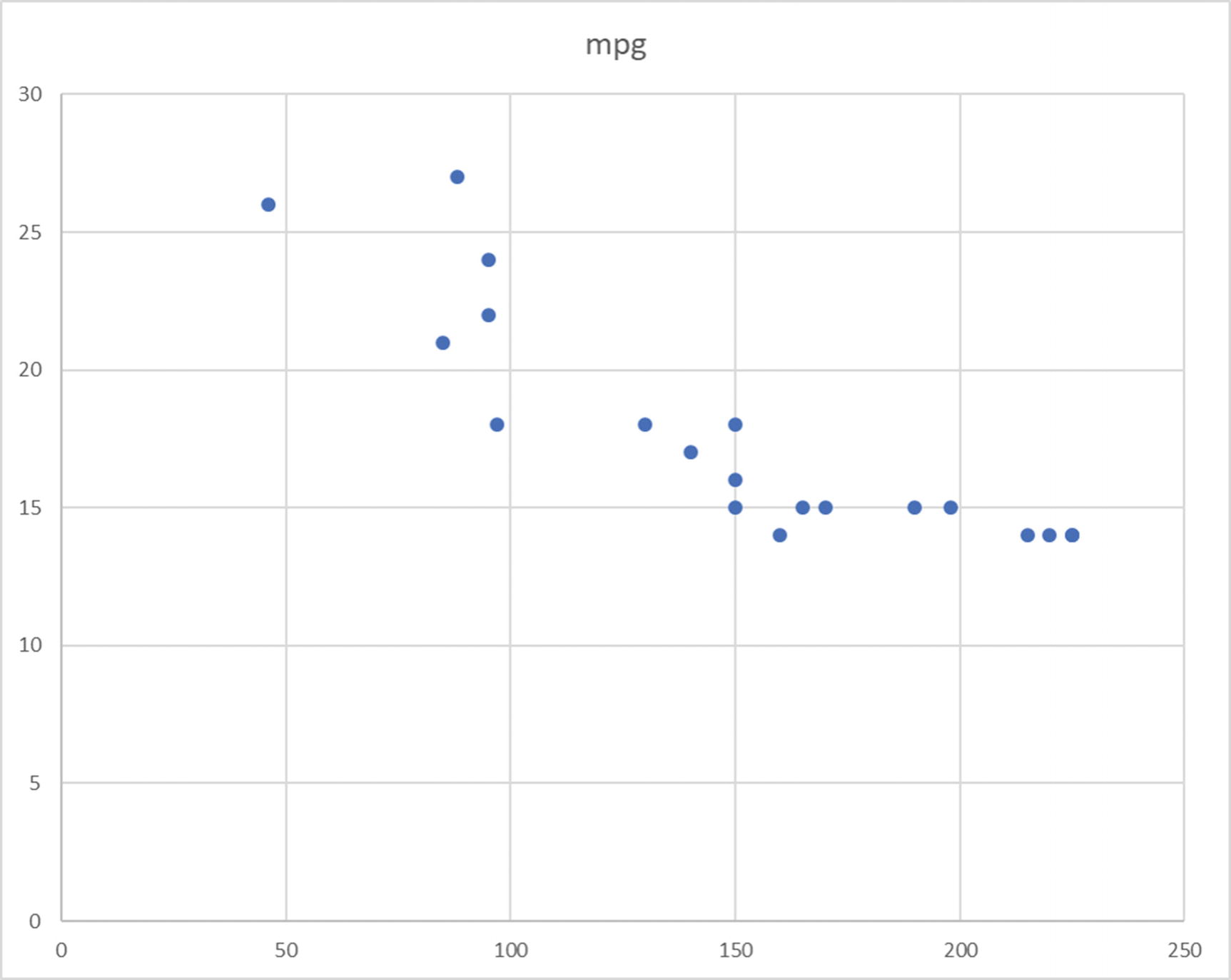
A scatter plot with horsepower on the x-axis and MPG on the y-axis
Model
Now if we carefully draw a line so that it passes through as many dots as possible, we’ll arrive at what looks like Figure 10-4a. This line represents our model. Yes, in linear regression this simple line is the model; the chart represents linear regression since we have drawn a straight line.
Predicting MPG values for unknown horsepower is now easy. In Figure 10-4a, we can see that there does not seem to be a corresponding MPG for horsepower 120. If we draw a dotted line at 120—perpendicular to the x-axis—the point where it intersects our model is the predicted MPG. As seen in Figure 10-4b, the predicted value is roughly 19.5.

(a) Creating our linear regression model by drawing a line (left). (b) Predicting a value using our model (right)
Training and Loss
The line we drew was just an approximation. The goal while drawing the line—in order to create a model—is to ensure it is not far away from most of the dots. In more technical words, the goal of plotting a model is to minimize the loss. But what is loss?

Loss is the vertical distance between actual and predicted target values

Thus, we define training as the iterative process of minimizing loss. That is, plotting and replotting the model until we arrive at a reasonably low value of MSE (overall loss). As with plotting model and calculating loss, there are several well-established ways to minimize overall loss. Stochastic Gradient Descent (SGD) is a common mathematical technique to iteratively minimize loss and, thus, train a model.
Where Do We Go From Here?
That’s it! This is all you needed to know about the internals of ML. Suddenly, the innocuous high-level terms you’d been hearing since Chapter 1 seem too mathematical. But if you have followed us up until now and understood most of ML internal concepts, congratulations! You have unlocked some confidence in getting started with an ML framework.
What open source ML frameworks, such as Tensorflow and scikit-learn, do is they provide you with ready-made methods to create a model, calculate loss, and train the model. However, you are required to have good working knowledge of cleansing data, picking features, and evaluating a trained model, among other things—all of which again require a decent hold on statistics and mathematics. An ML framework just makes dealing with multiple algorithms and multi-feature scenarios easier.
Azure Machine Learning Studio takes ease-of-use of ML a bit further by automating all of the above, while still giving expert ML engineers and data scientists control over the underlying processes.
Problems that ML Solves
Machine learning has literally unlocked an infinite amount of possibilities to get things done by machines that could not be done using traditional programming techniques. If we start listing down all the problems that ML can solve, we’ll run out of paper very soon. Fortunately, all these problems can be categorized into a handful of problem types. Let’s explore the most common types.
Classification
Identifying whether something is of type X or Y is a very common ML task. Humans gain the ability to discern various types of objects at a very early age. We can look at an animal with our eyes and instantly say, “it’s a dog.” So easy for a human, so humungous a task for a computer.

Multi-class classification to identify the kind of animal. For each class, hundreds of images are used to train the computer
Classification problems appear in two varieties—two-class (is it X or Y?) and multi-class (what kind is it?). Given an IoT device’s age, average temperature, and wear and tear, will it fail in the next three days (yes or no)? Is this a two-legged animal or a four-legged animal? These are two examples of two-class classification problems. Examples of multi-class classification are detecting the type of animal and species of a dog. In both examples, our system would need to be trained with several different animal types and dog species respectively, each animal type or dog species representing one class.
Who tells a computer what picture is a dog or a cat in the first place? Short answer—humans. Each picture is manually tagged with the name of the class it represents and supplied to the computer. This process is called labeling, and the class name supplied with training data is called a label.
Regression
This type of supervised learning (more on this later) is used when the expected output is continuous. Let’s see what we mean by output being continuous. We read about regression earlier in the section called “A Quick Look at the Internals”. You now know that regression uses past data about something to make predictions about one of its parameters.
For example, using a car’s horsepower-mileage data we could predict mileages (output) for unknown horsepower values. Since mileage is a variable, changing value—varies as per horsepower, age, cylinders, etc. even for the same car—it is said to be continuous. The opposite of continuous is discrete. Parameters such as car’s color, model year, size, etc. are discrete features. A red-colored car will always be red, no matter what its age, horsepower or mileage.
Based on what you just learned about output types, can you guess the output type classification deals with? If you answered discrete, you were absolutely correct.
Regression problems are very common, and techniques to solve such problems are frequently used by scientific communities in researches, enterprises for making business projects, and even newspapers and magazines to make predictions about consumer and market trends.
Anomaly Detection
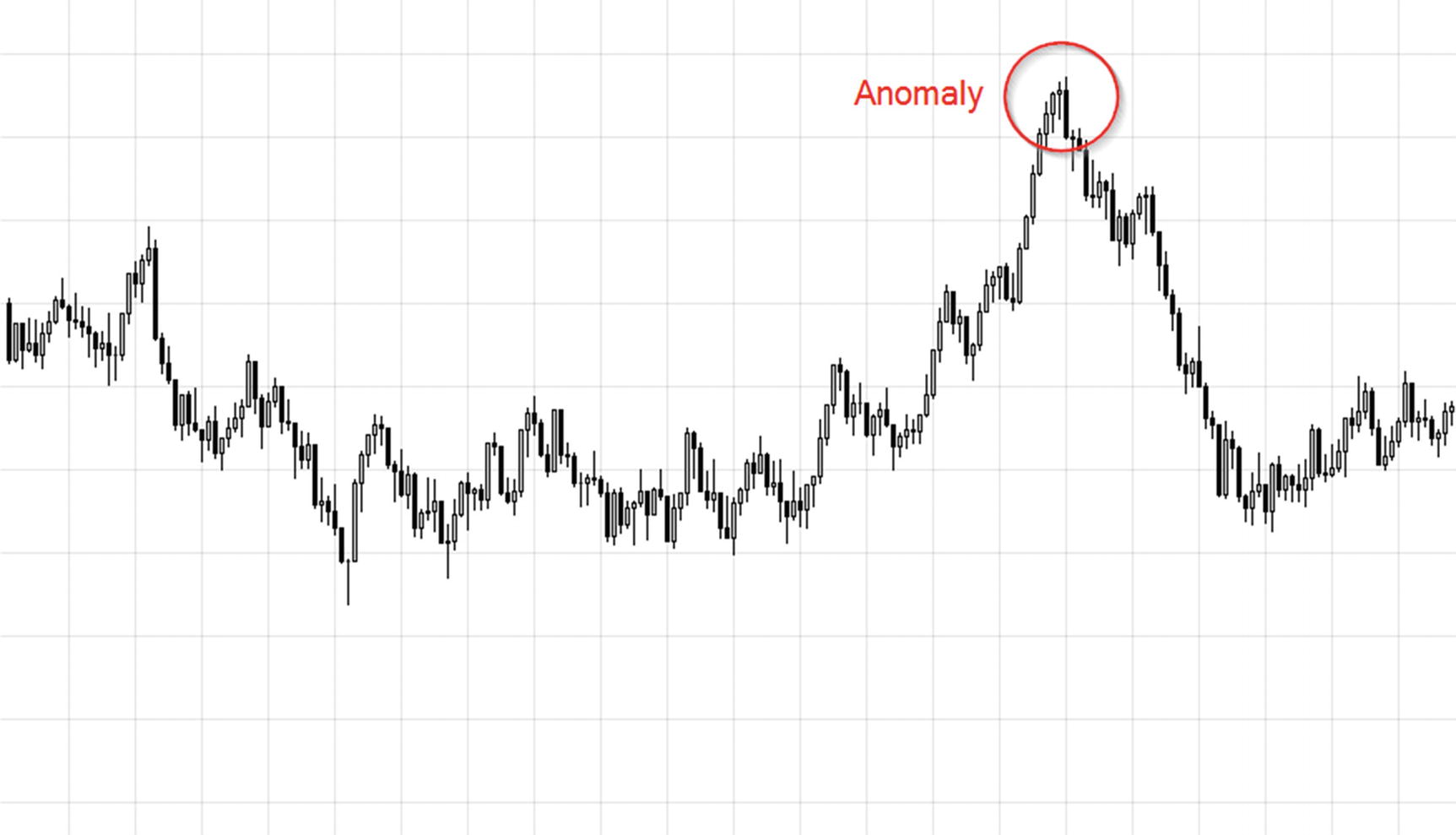
Abnormal point in an otherwise consistent trend
One of the most common anomaly detection use cases is detecting unauthorized transactions for a credit card. Consider this—millions of people use credit cards on a daily basis, some using them multiple times in a day. For a bank that has hundreds of thousands of credit card customers, the amount of daily data generated from card use is enormous. Searching through this enormous data, in real time, to look for suspicious patterns is not a trivial problem. ML-based anomaly detection algorithms help detect spurious transactions (on a stolen credit card) in real time based on customer’s current location and past spending trends.
Other uses cases for anomaly detection include detecting network breaches on high-volume websites, making medical prognoses based on real-time assessment of a patient’s various health parameters, finding out hard-to-find small or big financial frauds in banks, etc.
Clustering

Clustering allows you to organize data into criteria-based clusters for easy decision-making
Types of Machine Learning
After having learned what machine learning is—including a quick dive into its internal details—and the problems ML can solve, let’s take a quick look at the various types of ML. There really are only three types, based on how training is done.
Supervised Learning
Here, the training data is labeled. For a language detection algorithm, learning would be supervised if the sentences we supply to the algorithm are explicitly labeled with the language it’s written in: sentences written in French and ones not in French, sentences written in Spanish and ones not in Spanish, and so on. As prior labeling is done by humans, it increases the work effort and cost of maintaining such algorithms. So far, this is the most common form of ML as with it we get more accurate results. Classification, regression, and anomaly detection are all forms of supervised learning.
Unsupervised Learning
Here, the training data is not labeled. Due to a lack of labels, an algorithm cannot, of course, learn to magically tell the exact language of a sentence, but it can differentiate one language from another. That is, through unsupervised learning an ML algorithm can learn to see that French sentences are different from Spanish ones, which are different from Hindi ones and so on. Similarly, another algorithm can differentiate people who like Tom Hanks from those who like George Clooney and so on, and, thus, form clusters of people who like the same actor. Clustering algorithms are a form of unsupervised learning.
Reinforcement Learning
Here, a machine is not explicitly supplied training data. It must interact with the environment in order to achieve a goal. Due to a lack of training data, it must learn by itself from the scratch and rely on a trial-and-error technique to take decisions and discover its own correct paths. For each action the machine takes, there’s a consequence, and for each consequence it is given a numerical reward. So, if an action produces a desirable result, it receives “good” remarks. And if the result is disastrous, it receives “very, very bad” remarks. Like humans, the machine strives to maximize its total numerical reward—that is, get as many “good” and “very good” remarks as possible by not repeating its mistakes.
This technique of machine learning is especially useful when the machine has to deal with very dynamic environments, where creating and supplying training data is just not feasible. For example, driving a car, playing a video game, and so on. Reinforcement learning can also be applied to create AIs that can create drawings, images, music, and even songs on their own by learning from examples.
Azure Machine Learning Studio
There are multiple ways to create ML applications. We saw the mathematics behind linear regression in the section “A Quick Look at the Internals” earlier. One could write code implementation for linear regression by themselves. That would not only be time-consuming but also potentially inefficient and bug-ridden. ML frameworks, such as Tensorflow, make things simpler by offering high-level APIs to create custom ML models, while still assuming a good understanding of underlying concepts. Azure ML Studio offers a novel and easier approach to create end-to-end ML solutions without requiring one to know a lot of data science or ML details, or even coding skills.

Workflow of an ML solution in Azure ML Studio
- 1.
Import data. The very first thing you do in ML Studio is import your data on which machine learning is to be performed. ML Studio supports a large variety of file formats, including Excel sheets, CSV, Hadoop Hive, Azure SQL DB, blob storage, etc.
- 2.Preprocess. Imported raw data may not be straight-away ready for ML analysis. For instance, in a tabular format data structure some rows may be missing values for one or more columns. Similarly, there may be some columns for which most rows do not have a value. It may be desirable to remove missing data to make the overall input more consistent and reliable. Microsoft defines three key criteria for data:
- a.
Relevancy—All columns (features) are related to each other and to the target column.
- b.
Connectedness—There is zero or minimal amount of missing data values.
- c.
Accuracy—Most of the rows have accurate (and optionally precise) data values.
- a.
- 3.
Split data. Machine learning (in general) requires data to be split into two (non-equal) parts—training data and test data. Training data is used by an ML algorithm to generate the initial model. Test data is used to evaluate the generated model by helping check its correctness (predicted values vs values in test dataset).
- 4.
Train Model . An iterative process that uses a training dataset to create the model. The goal is to minimize loss.
- 5.
Evaluate Model. As mentioned, post initial model creation test data is used to evaluate the model.
Tip
It is possible to visualize data at each step of the process. Azure ML Studio provides several options for data visualization, including scatterplot, bar chart, histogram, Jupyter Notebook, and more.
Picking an Algorithm
The most crucial step in an ML workflow is knowing which algorithm to apply after importing data and preprocessing it. ML Studio comes with a host of built-in algorithm implementations to pick from. Choosing the right algorithm depends on the type of problem being solved as well as the kind of data it will have to deal with. For a data scientist, picking the most suitable one would be a reasonably easy task. They may be required to try a couple of different options, but at least they will know the right ones to try. For a beginner or a non-technical person, it may be a daunting task to pick an algorithm.
List of Algorithms Available in Azure ML Studio
Problem | Algorithm(s) |
|---|---|
Two-class classification | Averaged Perceptron, Bayes Point Machine, Boosted Decision Tree, Decision Forest, Decision Jungle, Logistic Regression, Neural Network, Support Vector Machine (SVM) |
Multi-class classification | Decision Forest, Decision Jungle, Logistic Regression, Neural Network, One-vs-All |
Regression | Bayesian Linear Regression, Boosted Decision Tree, Decision Forest, Fast Forest Quantile Regression, Linear Regression, Neural Network Regression, Ordinal Regression, Poisson Regression |
Anomaly detection | One-class SVM, Principal Component Analysis-based (PCA) Anomaly Detection |
Clustering | K-means Clustering |
Using Azure ML Studio to Solve a Problem
Time to solve a real-world problem with machine learning!
Asclepius Consortium wants to use patient data collected from various IoT devices to reliably predict whether a patient will contract diabetes. Timely detection of diabetes can be effective in proactively controlling the disease.
This problem, which can also be stated as “will the patient contract diabetes?,” is a two-class classification problem since the output can be either yes (1) or no (0). To be able to make any sort of predictions, we will, of course, need a lot of past data about real diabetes cases that can tell us which combination of various patient health parameters led to diabetes and which did not.
Let’s start.
Note
This problem can also be solved using linear regression. But as the output will always be either 0 or 1, rather than a more continuous value such as the probability of contracting diabetes, it’s best solved with a classification algorithm. During the course of your learning and experimenting with machine learning, you will come across a lot of problems that can be solved using more than one technique. Sometimes picking the right technique is a no-brainer, at other times that requires trying out different techniques and determining which one produces the best results.
Signing Up for Azure ML Studio
Using Azure ML Studio does not require a valid Azure subscription. If you have one, you can use it to unlock its full feature set. If you don’t, you can use your personal Microsoft account (@hotmail.com, @outlook.com, etc.) to sign into ML Studio and use it with some restrictions. There’s even a third option—an eight-hour no-restrictions trial that does not even require you to sign in.
Visit https://studio.azureml.net/ , click the Sign Up Here link, and choose the appropriate access. We recommend going with Free Workspace access that gives you untimed feature-restricted access for free. This type of access is sufficient to allow you to design, evaluate, and deploy the ML solution that you’ll design in the following sections. If you like ML Studio and want to try out restricted features and increase storage space, you can always upgrade later.
Choose the Free Workspace option and log into ML Studio. It may take a few minutes for Studio to be ready for first-time use.
Creating an Experiment
An ML solution in Studio is called an experiment. One can choose to create their own experiment from scratch or choose from dozens of existing samples. Apart from the samples that ML Studio provides, there is also Azure AI Gallery ( https://gallery.azure.ai/ ) that has a list of community-contributed ML experiments that you can save for free in your own workspace and use them as starting point for your own experiments.
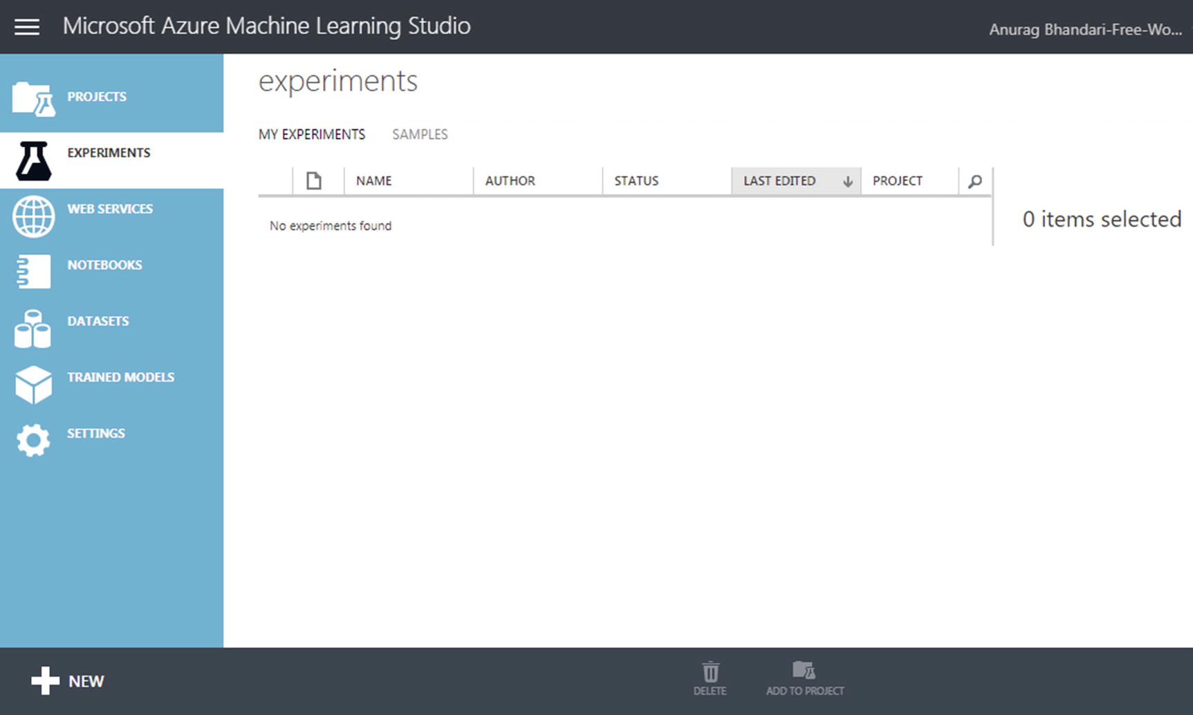
Experiments tab in a new Azure ML Studio workspace
Let’s create a new experiment from scratch in order to better understand the various components in an ML workflow, and how to set them up correctly. Click the New button in bottom-left and choose Experiment ➤ Blank Experiment. After your new experiment is created and ready, give it an appropriate name, summary, and description. You can use the name—Diabetes Prognosis—that we used in our own experiment.
Importing Data
Data is the most important part of a machine learning solution. The very first thing to do is import data that will help us train our model. To be able to predict diabetes in a patient, we need data from past cases. Until we have a fully-functional, live IoT solution that captures from patients health parameters relevant to diabetes, we need to figure out another way to get data.
Fortunately, there are online repositories that provide access to quality datasets for free. One such popular option is University of California, Irvine (UCI) Machine Learning Repository ( https://archive.ics.uci.edu/ml/ ). This repository is a curated list of donated datasets concerning several different areas (life sciences, engineering, business, etc.) and machine learning problem types (classification, regression, etc.). Among these datasets, you will find a couple of options for diabetes. You can download a dataset from here and later import it inside ML Studio, which provides support for importing data in a lot of formats such as CSV, Excel, SQL, etc.
Alternatively, you can simply reuse one of the sample datasets available inside ML Studio itself, some of which are based on UCI’s ML repository datasets. Among them is one for diabetes, which we will be using for in this experiment.

Importing sample data in an ML Studio experiment
It’s a good idea to explore what’s inside the dataset. That will not only give you a view of the data that Studio will be using for training, it will also help you in picking the right features for predictions. In experiment canvas, right-click the dataset and select dataset ➤ Visualize. You can also click the dataset’s output port (the little circle at bottom-middle) and click Visualize.
Preprocessing Data
This diabetes dataset has 768 rows and 9 columns. Each row represents one patient’s health parameters. The most relevant columns for our experiment include “Plasma glucose concentration after two hours in an oral glucose tolerance test” (represents sugar level), “Diastolic blood pressure,” “Body mass index,” and “age”. The Class Variable column indicates whether the patient was diagnosed with diabetes (yes or no; 1 or 0). This column will be our target (output), with features coming from other columns.
Go through a few cases, analyze them, and see how various health parameters correlate to the diagnosis. If you look more carefully, you will see that some rows have a value of zero for columns where 0 just doesn’t make sense (e.g., body mass index and 2-hour serum insulin). These are perhaps missing values that could not be obtained for those patients. To improve the quality of this dataset, we can either replace all missing values with intelligent estimates or remove them altogether. Doing the former would require advanced data science skills. For simplicity, let’s just get rid of all rows that have missing values.
Notice that the 2-Hour Serum Insulin column appears to have a large number of missing values. We should remove the entire column to ensure we do not lose out on a lot of rows while cleaning our data. Our goal is to use as many records we possibly can for our trained model to be more accurate.
Removing Bad Columns
From the left sidebar, go to Data Transformation ➤ Manipulation and drag-and-drop Select Columns in Dataset onto the canvas, just below the dataset. Connect the dataset’s output port with the newly added module’s input port by dragging the former’s output port toward the Select Columns module’s input port. This will draw an arrow pointing from dataset to the module.
Note
Modules in Azure ML Studio have ports that allow data to flow from one component to another. Some have input ports, some have output ports, and some have both. There are a few modules that even have multiple input or output ports, as you’ll see shortly.

Excluding a column in Azure ML Studio
As a hint to yourself, you can add a comment to a module about what it does. Double-click the Select Columns module and enter the comment Exclude 2-Hour Serum Insulin.
Renaming Columns
The default names of columns in our dataset are too long and descriptive. Let’s simplify the column names. Search for and add the Edit Metadata module in canvas, just below Select Columns. Connect it to the module above. In module’s properties pane, click Launch Column Selector and select all columns except 2-Hour Serum Insulin. Coming back to the properties pane, add the following new names in the New Column Names field, leaving all other fields unchanged:
Click the Run button to run your experiment. After it’s finished running, all modules that ran successfully will have a green check mark. At this point, right-click the Edit Metadata module and visualize the data. You should see the same dataset with renamed columns.
Removing rows with Missing Values
This is usually done using the Clean Missing Data module, which can remove rows where all or certain columns have no specified values. Since our data has no explicit missing values, this module will not work for us. We need something that can exclude rows where certain columns are set to 0 (e.g., glucose_level, bmi, etc.).
Search for and add the Apply SQL Transformation module in canvas, just below Edit Metadata. Connect its first input port to the module above. Enter the following query in the SQL Query Script field in the module’s properties pane:
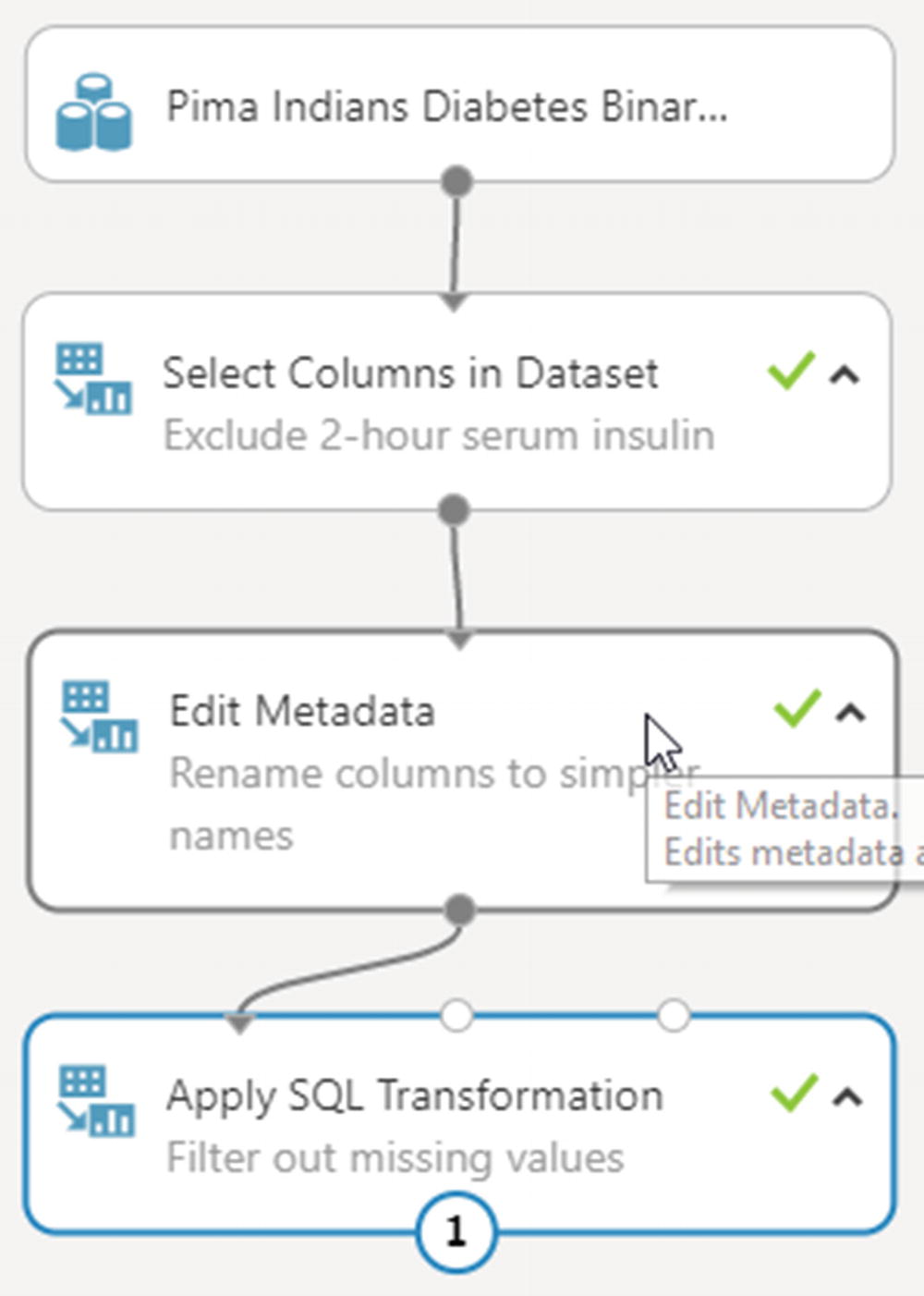
Experiment canvas after performing data preprocessing
Defining Features
Our data is now ready to be used for training. But before we perform training, we need to handpick relevant columns from our dataset that we can use as features.
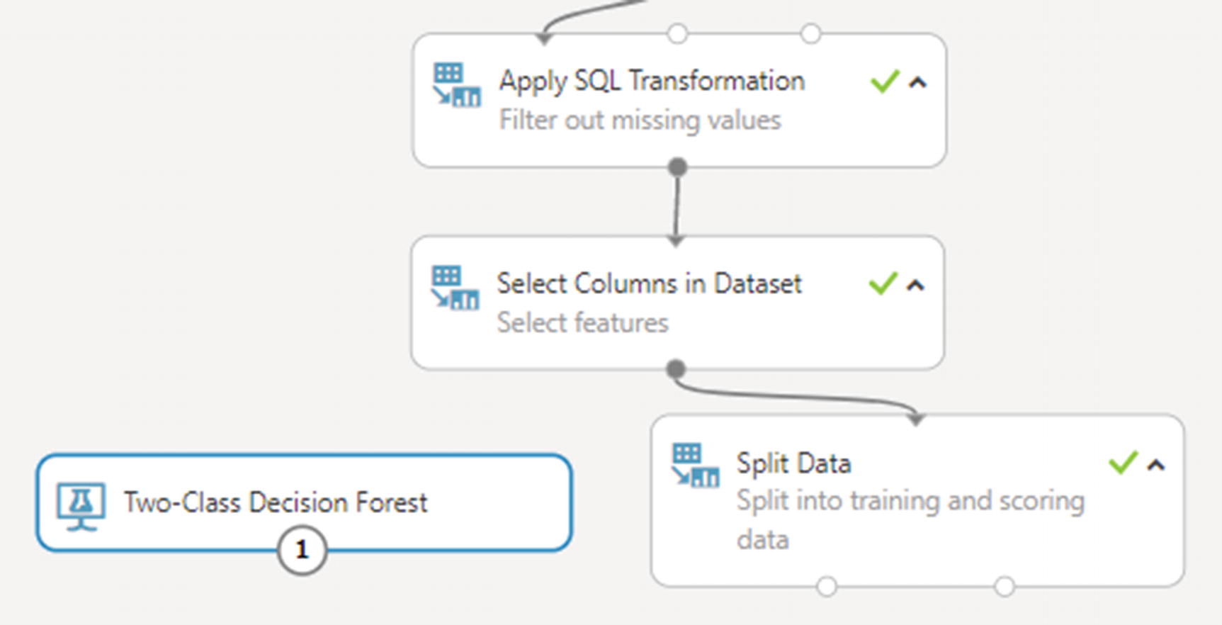
Search for and add a second Select Columns in Dataset module in canvas, just below Apply SQL Transformation. Connect it to the module above. From column selector, choose glucose_level, diastolic_blood_pressure, triceps_skin_fold_thickness, diabetes_pedigree_function, bmi, and age.
Splitting Data
As discussed earlier in the chapter, a dataset should be divided into two parts—training data and scoring data. While training data is used to actually train the model, scoring data is reserved for later testing the trained model to calculate its loss.
Search for and add the Split Data module in canvas, just below the second Select Columns module. Connect it to the module above. In its properties page, set 0.75 as the value for Fraction of Rows in the First Output Dataset. Leave all other fields as such. Run the experiment to ensure there are no errors. Once it’s completed, you can visualize the Split Data module’s left output port to check training data and right output port to check scoring data. You should find both in the ratio 75-25 percent.
Applying an ML Algorithm
With data and features ready, let’s pick an algorithm from one of the several built-in algorithms to train the model. Search for and add the module called Two-Class Decision Forest in canvas, just to the left of Split Data. This algorithm is known for its accuracy and fast training times.
With data and algorithm ready; we are all set to perform the training operation
Training the Model
Search for and add the module called Train Model in canvas, just below the algorithm and Split Data modules. Connect its left input port to the algorithm module and its right port to Split Data’s left output port.
From its properties pane, select the Diabetic column. Doing so will set it as our model’s target value. Run the experiment. If all goes well, all modules will have a green checkmark. Like data, you can visualize a trained model as well, in which case you will see the various trees constructed as a result of the training process.
Scoring and Evaluating the Trained Model
Training using the selected algorithm takes only a few seconds to complete. Training times are directly proportional to the amount of data and selected algorithm. Despite Azure ML Studio’s state-of-the-art implementations of ML algorithm, you should not be straight-away satisfied with the generated model. Just as with a food recipe one should taste a finished dish to determine if any modifications are necessary to make it more tasty, with a trained model one should score and evaluate it to see check certain parameters that can help ascertain if any modifications are necessary, for example changing the algorithm.
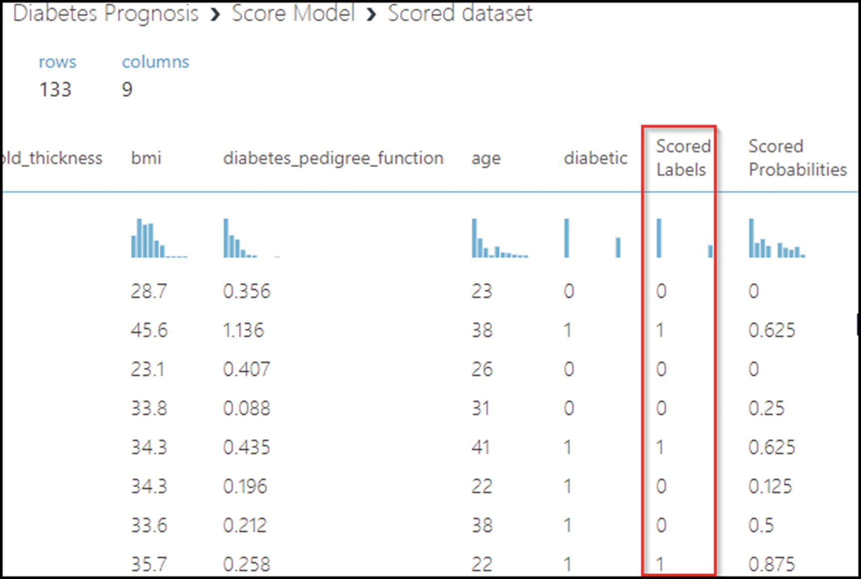
Visualizing scored data in Azure ML Studio
As you can confirm from the figure, scoring is performed with the 25% output of Split Data module. Values in the Diabetic column represent the actual values in the dataset, and values in the Scored Labels column are predicted values. Also note a correlation between the Score Labels and Scored Predictions columns. Where probability is sufficiently high, the actual and predicted values are the same. If actual and predicted values match for most rows, you can say our trained model is accurate. If not, try tweaking the algorithm (or replacing it altogether) and running the experiment again.
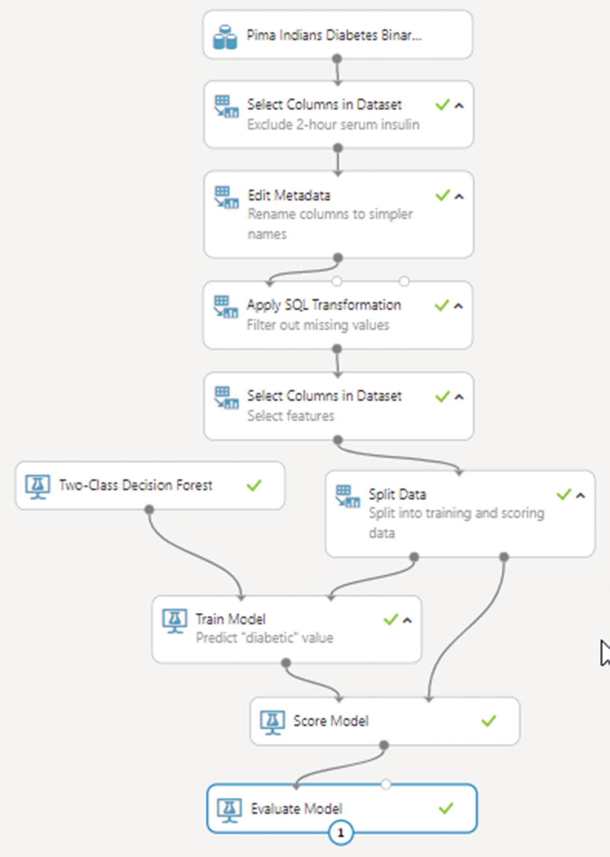
Final preview of a two-class classification ML solution
Deploying a Trained Model as a Web Service
Now that we have a trained and tested model, it’s time to put it to real use. By deploying it as a web service, we’ll give end-user software applications an option to programmatically predict values. For example, we use the diabetes prediction model’s web service in our IoT solution backend or with Azure Stream Analytics to predict diabetes in real time.
Choose the Set Up Web Service ➤ Predictive Web Service option. This will convert our current experiment to what is called a Predictive Experiment. After the conversion is complete, your experiment will have two tabs—Training Experiment and Predictive Experiment—with the former containing the experiment that you set up in the previous sections and the latter containing its converted version that will be used with web service.
While in Predictive experiment tab, click the Run button. Once running completes successfully, click Deploy Web Service. You will be redirected to a new page, where you will find details about the deployed web service. It will also have an option to test the web service with specified values for features. Refer ML Studio’s documentation at https://bit.ly/2Eincl7 to learn more about publishing, tweaking, and consuming a predictive web service.
Recap
Machine learning fundamentals—the what and why
Differences between ML and data science
Brief overview of ML internals—model and training
The problems ML solves—classification, regression, etc.
Types of ML—supervised, unsupervised, and reinforcement
Azure Machine Learning Studio
Creating and deploying your own ML solution
Congratulations! You are now officially AI 2.0-ready. In this book, you learned a host of new technologies that will separate you from your peers, and help you design the next generation of software applications. We encourage you to learn about each new technology in more detail and practice as much as possible to improve your hands-on skills.