Technologies for Long-Term Applications
Abstract
Emergency response and humanitarian aid organizations need to supply water treatment devices in a cost-effective manner that also creates a high-quality effluent acceptable for human consumption. Certain technologies are more applicable in a long-term emergency situation than acute, short term applications. Long-term emergency response water treatment devices are typically more expensive, provide a higher effluent flow and quality, and take longer to set up, maintain, and operate than do water treatment devices provided during a short-term, acute, emergency response. The technologies discussed for long-term applications include natural filtration, packaged filtration units, pressurized filtration units, and small-scale systems.
5.1 Slow Sand Filtration
Slow sand filtration (SSF) is a low-cost, yet effective treatment option for removing microbes in source water. It has helped tremendously in stopping the spread of gastrointestinal diseases in developing countries. SSF was first employed for municipal use in the 1850s in Great Britain (Logsdon et al., 2002), then was implemented in other European countries and eventually the United States in 1885 (Huisman and Wood, 1974). SSF saved hundreds of lives during the 1892 cholera epidemic in Germany, particularly in Altoona, which is downstream of Hamburg (Logsdon et al., 2002). This is one of the many cases that have demonstrated the efficacy of SSF even though the science of microbiology was still developing at that time.
Untreated fresh water (from rivers, lakes, rain water, etc.) is fed to a sand bed that is typically 0.5 m in depth or deeper in some cases. The water percolates down through the sand because of gravity. A certain amount of water stays on the surface of the sand at all times, creating a pond-like environment. With time, a biolayer (often referred to as a schmutzdecke) grows on the top layer of sand particles that are under water. It is typically reddish brown and has a slimy film. This layer acts as a preliminary filter that removes fine colloidal particles and organic matter from the feed water (ITACA, 2005). The biolayer also helps to remove bacteria and pathogens through sorption, predation, and other mechanisms.
5.1.1 Removal Efficiency
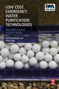
Typically, water turbidity is reduced to less than 1 NTU in municipally operated SSF units. Gottinger et al. (2011) have compiled the removal efficiency statistics of SSF units for various contaminants, including microbial and chemical as well as physical impurities present in source water. In well-operated systems, a significant amount of these contaminants are removed (Table 5.1). What is striking about this data is that almost all Giardia cysts are removed and up to 4 log removals of Cryptosporidium oocysts is achieved. More than 2 logs of fecal bacteria removal is achieved. Polio virus removal of up to 5 logs is attained. Trihalomathane (THM) precursor removal is shown to be less than 25%.
Table 5.1
Literature Data on the Efficacy of Slow Sand Filtration on Removal of Microbial, Chemical, and Physical contaminants in Source Water
| Parameter | Removal Efficiency or parameter value in effluent | Reference(s) |
| Turbidity | < 1 NTU | Visscher (1990), Galvis et al. (1998) in Cleary (2005) |
| True color | 25-40% | Galvis et al. (1998) in Cleary (2005) |
| 30-100% | Visscher (1990) | |
| Organic matter | 60-75% | Visscher (1990) |
| UV absorbance (254 nm) | 3-35% | Galvis et al. (1998) in Cleary (2005) |
| THM precursors | < 25% | Galvis et al. (1998) in Cleary (2005) |
| Viruses | Almost complete removal | Visscher (1990) |
| Fecal coliforms | 95-100% to 99-100% | Visscher (1990) |
| Standard plate count bacteria | 96% | Bellamy et al. (1985a) |
| Giardia cysts | Almost 100% | Bellamy et al. (1985a) |
| Cryptosporidium oocysts | 99.8-99.99% | Various citations in Logsdon et al. (2002) |
| Poliovirus | 99.997% average | Poynter and Slade (1977) in Logsdon et al. (2002) |
| Iron and manganese | 30-95% | Visscher (1990) |
(from Gottinger et al., 2011)
Note: THM = trihalomethane.
5.1.2 Construction
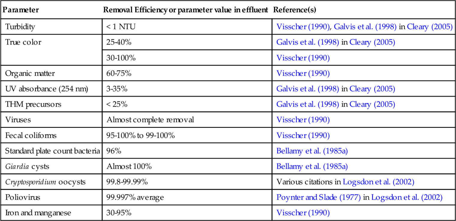
For a municipal or public water supply, the construction of SSF is quite elaborate, and standard texts and design manuals or handbooks are available (Randtke and Horsley, 2012). Figure 5.1 shows a diagram of a slow sand filter typically used to treat public water supplies.
Typically, each filter is a concrete box with appropriate pumps, pipes, underdrains, and baffles. As shown in the figure, raw water is fed to the top of the filers from one side of the wall. The sand in the filter sits above a gravel bed that acts as support as well as a drain. The water level in the filter bed is adjusted by a weir just outside the wall so that there is a small depth of water just sitting on the top of the sand bed. This allows the schmutzdecke to grow. The overflow from the weir is collected as filtrate. It may be further treated to comply with local, state, and federal water quality regulations for public water utilities.
The town of Falls City, Oregon, has a population of about 950. It built an SSF unit at a cost of about $1.5 million (by SCG Slayden of Slayton, OR) that included the costs of three filter beds; pumps; piping; a covered chlorine contact basin and clear well; and the adjacent building for controls, monitoring, and office space (Figure 5.2). The source water comes from a creek.

While SSF has been effective in treating large amounts of raw water from streams, lakes, or ponds, its construction may take some time, and, thus, large, permanent SSF systems may not be effective in emergency situations. Immediately after disasters, portable SSF can be set up in plastic barrels or brick tanks with appropriate piping so that potable water can be produced in a week or two. Community-scale or smaller (one or a few houses) systems can be set up easily.
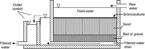
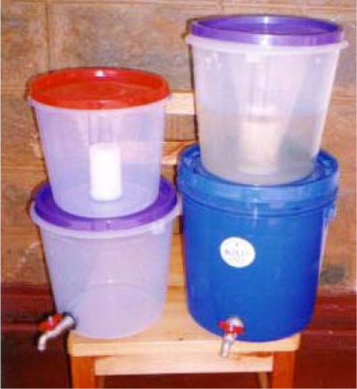
Using drums or barrels, small portable SSF units can be set up for household use. Larger plastic tanks can be used for community-scale operations (Figure 5.3). Typically, the filter should be at least 0.5 m deep (ITACA, 2005). The mean diameter of sand typical sand particle size is between 0.15 and 0.35 mm (ITACA, 2005), with a uniformity coefficient of less than 5 (Logsdon et al., 2002). The filters operate most effectively at a continuous and constant flow rate of 0.1-0.3 m/h (or m3/h/m2) or 100-300 L/h per m2 of filter media (Logsdon et al., 2002). Generally, smaller sand size and slow flow rates make for the best removal efficiencies (Kubare and Haarhoff, 2010).
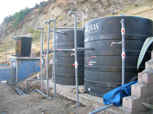
For households and small communities, plastic barrels that are 55-gallon capacity (Figure 5.4) can be used to construct the SSF system. These barrels are typically 88 cm tall and 57 cm diameter. In order to study the effectiveness of the removal of particles and other contaminants, it is best to install sampling ports at various depths, starting at a depth of 2 cm below the surface of the sand. A support medium (typically 5 cm of coarse gravel below 2 cm of fine gravel) is used below the sand bed. The underdrain subsystem lies in the gravel. After packing the sieved sand to the desired depth, the sand is saturated with clean water and then back flushed for several hours to remove fine particulates. Then the feed water is supplied to the top of sand. This can be done manually through a siphon mechanism or from an overhead tank. The SSF should have an overflow system to maintain a constant head of water. The filtered water may be additionally treated using silver-impregnated activated carbon filters or UV light (or both).

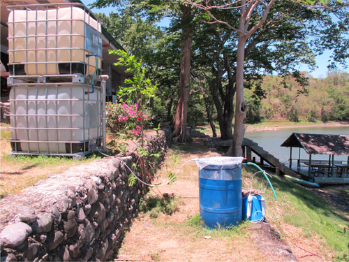
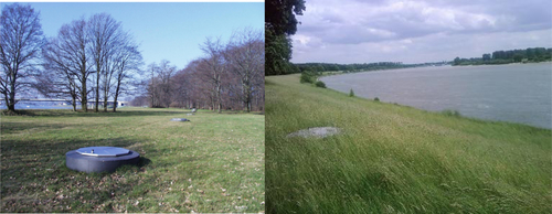
The authors evaluated the use of SSF for small community water supplies in the Philippines following disasters. In a demonstration study, they used source water from a reservoir in Fort Magsaysay in the Philippines. They used tanks that could be filled manually or with a small pump if power was available to store the source water from the reservoir, and they used standard barrels that are 55-gallon capacity to make the filters. Figure 5.5 shows such a unit near a reservoir.
A key component of the SSF is the schmutzdecke, often referred as the biolayer or zoological film. This reddish brown, slimy film acts as a preliminary filter that removes fine colloidal particles and organic matter from the raw feed water (ITACA, 2005). It consists of active bacteria, their wastes and dead cells, and partly assimilated organic matter. Within this film, bacteria derived from the raw water multiply selectively, and the deposited organic matter is metabolized as nutrients. The bacteria oxidize part of the food for energy to grow and reproduce (Huisman and Wood, 1974). Within 2-3 weeks, the schmutzdecke is fully developed and ripened, depending on the flow rate, the composition (organic matter present), the oxygen content, and the temperature of the raw water (ITACA, 2005). As water continues to pass through the filter, the schmutzdecke thickens, removing contaminants more efficiently. However, once the water passing through the filter slows below the desired flow rate (clogging), the schmutzdecke must be scraped and cleaned. After cleaning, it will take a few days to re-ripen (ITACA, 2005).
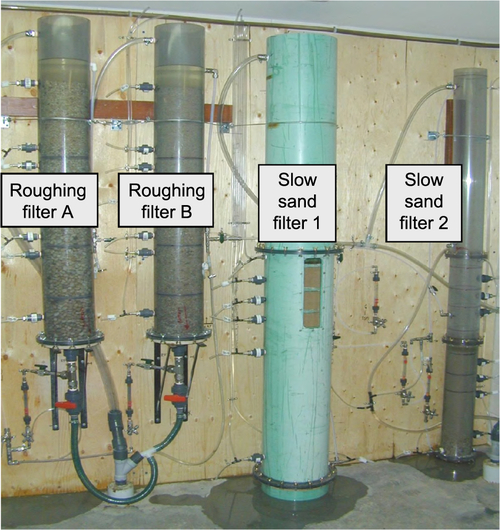
The quality of feed water affects effluent quality. Turbidity is a key water quality parameter that affects the performance of SSF units. High turbidity water coats the schmutzdecke with clay and colloidal particles. This diminishes the biological activity and leads to clogging of the sand surface. Ideally, the turbidity of the feed water should be between 10 and 20 NTU for the SSF to function properly. It can handle higher turbidity for a short time; however, exposure to high turbidity (20-30 NTU or higher) for extended periods will cause clogging and coating of the biolayer, thus reducing filtration effectiveness. Multistage filtration, where a roughing filter precedes an SSF and removes a certain amount of turbidity, can be useful during periods of high turbidity. Cleary (2005) studied the effect of a roughing filter on the removal of microbes during SSF of surface water. Roughing filters (Wegelin, 1983; Wegelin and Schertenleib, 1993) typically consist of gravel particles with diameters ranging from 20 to 4 mm and can be set up in vertical or horizontal flow configurations with variable depths/lengths. Vertical filters can be down-flow or up-flow. Cleary (2005) cites several sources to confirm that using a roughing filter increases the hydraulic loading to SSF (as much as 0.4-0.8 m/h). The primary processes affecting particle removal in roughing filters are gravity settling, interception, and diffusion. Galvis et al. (1996) tested up-flow and horizontal flow roughing filters using source water from a heavily polluted lowland river in Colombia. The turbidity, color, and fecal coliform counts for the source water were 15-1880 NTU, 24-344 true color units, and 7300-396,000 MPN/100 mL, respectively. The filters were 4.3 m long or deep, and the filtration velocity was 0.7 m/h. The removal rates for these parameters were 66.7%, 93.8%, and 95.6% for horizontal roughing filters, respectively. For the up-flow roughing filters, the removal rates for the same parameters were 80%, 97.9%, and 99.4%, respectively. Cleary (2005) set up a multistage filtration system, shown in Figure 5.6. A second configuration (Figure 5.7) was set up for comparison. Turbidity removal for the Pilot System 1 (Figure 5.6) during a period of about 4 months is shown in Figure 5.8. As shown in this figure, the effluent turbidity of the SSF was exceeded only once in response to a rain event at the end of March. Pilot System 2 (Figure 5.7) also performed well (see Figure 5.9) with only one incidence of turbidity reaching 1 NTU.

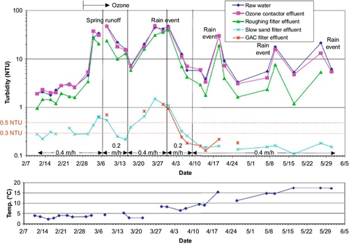
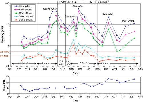
Because ozone was used as a pretreatment before the roughing filters in Pilot System 1, log removal of coliforms just after ozonation was between 2 and 3 logs. In Pilot System 2, it was less than 1 log after roughing filters, and total removal with the multistage filtration was between 2 and 3 logs.
El-Swaify (2013) studied the performance of household slow sand filters (within plastic barrels as shown in Figure 5.4) in parallel and in series. In parallel, two slow sand filters were subjected to differing flow rates to examine the effect of loading rate on the removal of drinking water contaminants. In series, two filters were run at a given flow rate to examine if the second filter further improved the filtration efficiency.
In the first parallel mode operation, the water through one filter (B1) had a flow rate of 0.035 m/h, and the water through the other filter (B2) had a flow rate of 0.07 m/h. The filters were run for 1 month. Turbidity, E. coli, and total coliforms were monitored in the influent and bottom effluent as well as posttreatment units. The posttreatment units included (a) UV treatment, (b) silver-impregnated activated carbon, and (c) charcoal made from local coconut shells. A Sun-Pure Ust-200 Ultraviolet System (Freshwater System, Greenville, SC) was used for on-line disinfection. The UV bulb was contained within a polypropylene chamber (5 cm internal diameter and 30 cm length) that had a stainless steel lining and a 0.625 cm inlet and outlet. The system allowed a flow rate of 3.6 liters per minute (lpm), with a dose of 30 mJ/cm2.
A second test was conducted to examine the effect of a sudden change in flowthrough on water quality. El-Swaify (2013) ran water through one filter at 0.025 m/h (B1) and water through another at 0.12 m/h (B2) in parallel operation. He ran those two filters for 14 days and then reversed the flows (high rate to low rate and vice versa [i.e., the new flow rate of B1 became the old flow rate of B2 and vice versa]). Posttreatment units attached to the filter were UV light and silver-impregnated activated carbon.
In series mode, El-Swaify ran the two filters at a flow rate of 0.1 m/h for 38 days. During the first 27 days, the turbidity of the feed water averaged around 5 NTU. After that, the feed water turbidity increased to about 23 NTU.
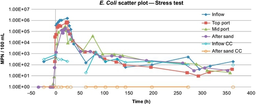
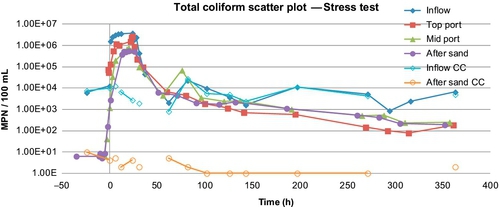
He also conducted a stress test on the two barrels in parallel configuration (B1 and B2), simulating the effect of a sewage spill in stream water to one barrel. The flow rate was 0.035 m/h (barrel B1), and the simulated spill lasted for 1 day. After that, normal stream water was fed to both the barrels for two more weeks. For barrel B2, no spill was simulated. The flush out effect was studied at the bottom of the barrel and at two sampling depths, 2 cm below the sand surface and 28 cm below.
Silver-impregnated activated carbon may be one possible postfiltration treatment. However, we have already pointed out that such units are not highly effective because the silver gets washed away with time and the carbon surface can become a site for bacterial growth. However, the granular activated carbon (GAC) helps to remove tastes and odors from drinking water.
UV light is another possible posttreatment mechanism. Especially in disaster-affected areas, UV systems can be powered by solar panels or car batteries. A solar panel can charge a deep cycle battery and keep a UV system running for years.
In the parallel mode study conducted by El-Swaify (2013), mentioned above, he used UV light, silver-impregnated GAC, and locally prepared charcoal from coconut shells. For series operation, he only used silver-impregnated GAC. For stress tests, no posttreatment devices were used. Figures 5.10 and 5.11 show the removal of turbidity and E. coli for the two flow rates (barrels B1 and B2). There was between 1 and 2 log reductions in E. coli after the sand. Barrel 1, which had a lower flow rate, showed better removal of E. coli (between 2 and 3 logs); however, the turbidity removal rates were not that different (81% for B1 vs. 78% for B2 in the first 24 days, and 83% and 76%, respectively, in the last 6 days). Logsdon et al. (2002)suggest operating at flow rates between 0.1 and 0.3 m/h. In this case, both B1 and B2 had lower flow rates than the minimum suggested.

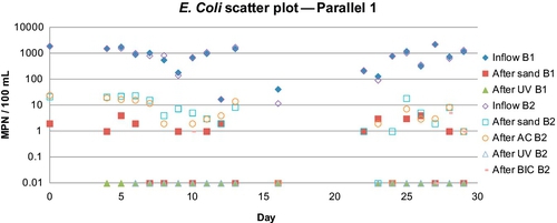
El-Swaify also found that, at low-flow rates, the biolayer did not fully form during the duration of the study (30 days) whereas, at the high flow rate, it took about 3 weeks for the biolayer to form. Although the formation of the biolayer was not complete in barrel B1, turbidity and bacteria were both steadily reduced. Thus, there must be a sufficient amount of flow and possibly nutrients so that the biolayer can form.
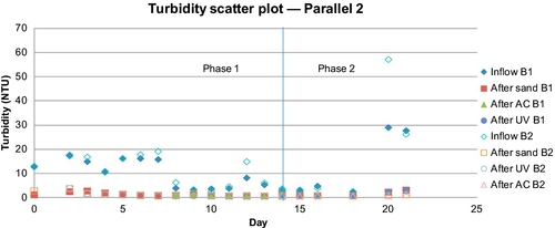
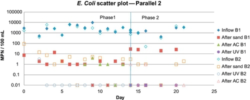
Figures 5.12 and 5.13 show the removal of turbidity and E. coli in the two parallel barrels where the flow rates were reversed after 2 weeks. While the removal in turbidity was not significant, even rising in the second half of the experiment, the removal of E. coli was affected by the changes in flow. For barrel B1, the increased flow rate in the second half of the experiment increased the effluent E. coli. Similarly, there was a drop in the E. coli for B2 when its flow rate was dropped from 0.07 to 0.035 m/h.
An interesting observation was made when the two barrels were run in series (but at the same flow rate). Overall, a higher removal of turbidity, total coliforms, and E. coli was observed in B1 compared to B2 (Figures 5.14 and 5.15).


It can be concluded from this simulation that when the feed water has normal turbidity (3-10 NTU), total coliforms (102-104 MPN/100 mL), and E. coli (101-103 MPN/100 mL), the first barrel sufficiently purifies the water. Because B1 removed the majority of the “food” (i.e., organic matter, bacteria) from the source water, B2 did not have enough nutrients to develop the biolayer. As a result, B1 formed a thick, healthy biolayer, while B2 did not form a biolayer at any time during the experiment. Under normal conditions, one SSF with a GAC column as a posttreatment device is a better option than two SSFs in series.
To improve the efficiency of the two barrels, B1 and B2 can be configured in parallel, maintaining each filter and establishing their respective biolayers. In the event of a stress condition, such as extended periods of heavy rainfall or a sewage spill, B1 and B2 can then be configured in series. Because of the high starting values of total coliforms (106-107 MPN/100 mL) and E. coli (105-106 MPN/100 mL) at these times, B1 will most likely shed a large amount of bacteria, which B2 will be able to fully remove. In a case of high turbidity (> 15 NTU), a prefiltration technique such as a roughing filter or natural settling should be employed to prevent clogging of the SSF.
The results of stress tests for turbidity and E. coli are shown in Figures 5.16 and 5.17. Figure 5.18 shows the concentrations of total coliforms in water samples collected from the same test. Figure 5.19 shows the removal efficiency for E. coli, coliforms, and turbidity with various posttreatment units.
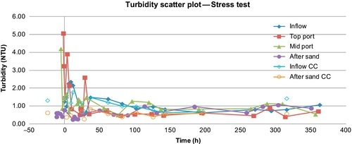
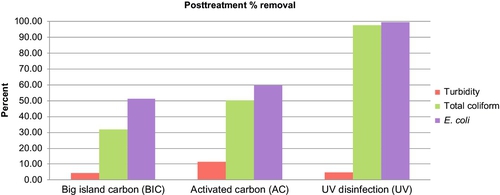
As shown in these figures, UV disinfection was most effective in reducing the coliforms and E. coli. Activated carbon reduced the turbidity by another 10%; however, its ability to remove coliforms of E. coli was between 50% and 60%. Also, as stated earlier, activated carbon units are not efficient in removing microorganisms.
It is clear that SSF can be viable a treatment technology for long-term applications at varying scales, from household drinking water needs to those of large communities. Additional research characterizing the microbial community structure and the ability of SSF to remove emerging chemicals such as pharmaceuticals, antibiotics, and endocrine-disruptors will be useful.
5.2 Packaged Filtration Units
Filters that use either micro- or ultrafiltration to purify water have been tested and can be used in emergency water treatment. These packaged filters are powered by either gravity or human suction. Because of this limitation, these filters produce only small volumes of water and are more appropriate for use by small families or individuals. However, because these devices are powered by gravity and suction of human mouth, they are relatively low cost and do not consume fuel so they can be used if no alternative power sources are available. Like most filtration devices, packaged filtration units require proper maintenance and operation to achieve effective bacterial and contaminant removal.
5.2.1 Candle Filter
The candle filter is one of the most researched and evaluated ceramic filters used to purify water. A candle filter is a filter that looks like an upside down candle. A candle filter is screwed into the bottom of the top bucket of a stacked bucket filtration system; see Figures 5.20 and 5.21. Water is poured into the top bucket, percolates through the ceramic candle, and is stored in the bottom bucket. The bottom bucket contains a spigot that can be opened for water consumption. The bottom bucket can generally store up to 20 L of water.

5.2.1.1 Materials, Manufacturing, and Removal Efficiency
Ceramic candle filters can be manufactured by professional companies or by locals. Local construction of these filters results in varied quality of the products, which affects the filtration system’s effectiveness, while professional products have a higher cost but result in a higher quality product. Local Indian companies make filters by mixing red, white, or black clay with water and sawdust or flour and then compressing it into a mold. The filter is heated in an oven to vaporize the sawdust to create open pores. Pore sizes of the ceramic candle filter range from less than 1 up to 5 μm, depending on the manufacturing techniques and materials used. These pore sizes are small enough to filter out bacteria and protozoa but too large to filter out viruses. However, viruses that have a charge can adsorb to filter surfaces, reducing the number of viruses in the treated effluent. Lab tests performed on locally made filters reveal that disease-causing pathogens are not always removed by candle filters because of cracks that allow water (and microbes) to find “paths of least resistance” and enter the effluent. Flow rates of locally made filters are very slow, ranging from 0.04 to 0.25 L/h.
Filters made by companies such as Katadyn, Hong Phuc, or Kisii (Dies, 2003) have been tested and found to be more efficient than locally made filters for bacterial removal, although they do not remove 99.9% of viruses. The Katadyn product uses a filter media impregnated with fine silver powder and GAC to improve the taste and smell of the drinking water. The Hong Phuc filter uses a diatomaceous earth filter, while the Kisii system offers a choice between a ceramic filter or a filter with GAC and silver. Flow rates for these manufactured systems are faster than the locally produced ceramic filters, ranging from 0.125 to 4 L/h (Dies, 2003).
5.2.1.2 Improve Filter Efficiency
To improve efficiency, different configurations of candle filters can be used. More than one candle filter can be inserted into the stacked bucket system in order to increase the flow rate of treated water. A candle filter manufactured by the Rural Water Development Program (RWD) offers a “jumbo” configuration of a five-candle system to schools and small hospitals.
Coating the filter in colloidal silver has been found to effectively remove microbes. Dies (2003) found that by coating the candle filters in silver, the microorganism log reduction value was increased by 1.15 and the E. coli log removal value (LRV) was increased by 0.85.
5.2.1.3 Maintenance
Candle filters require frequent maintenance. Because of particle build up and the resulting reduced flow rates, filters must be cleaned with a soft brush and clean water every 2 weeks (Dies, 2003). After successive cleanings, the ceramic candle tends to lose wall thickness and becomes less effective for removing microbes (Clasen and Boisson, 2006). The service life of candle filters vary, but they should be replaced every 6-12 months (Clasen and Boisson, 2006; Dies, 2003).
Ceramic candle filters are fragile and must be handled with care. Even the slightest crack will reduce the microbiological removal effectiveness of the device. Surveys of candle filter users noted that many people stopped using them because of breakage. Those who owned broken filters rarely bought a replacement filter and went back to using untreated water (Clasen and Boisson, 2006) whether replacement filters were available or not. Training, although not extensive, can promote proper maintenance and use of candle filters. Some shop owners who sell these filters teach consumers how to operate and maintain their new filters (Dies, 2003).
5.2.1.4 Cost
• Indian Company Manufacturers (1-2 candles, containers, spigot): $8-21
• Purchase of plastic buckets (instead of containers) to save money: $2.22 for buckets
• Nepal Filters: Terracotta clay containers with white kaolin filters for $4.07 each
• Or buy in bulk for $2.29 each
• Katadyn Filters (containers, spigot, filters): $160-190
• Hong Phuc Filter (containers, spigot, filters): $7.50
• Kisii Filters
• High rate filter: $12
5.2.2 Ceramic Disk Filter
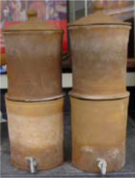
The disk filter is another ceramic filter used to purify water. A disk filter is a cylindrical ceramic filter that fits into the bottom of the top bucket of a stacked bucket filtration system; see Figures 5.22 and 5.23. These buckets can be made of terracotta, metal, or plastic. Water is poured into the top bucket, percolates through the ceramic disk, and is stored in the bottom bucket. The bottom bucket contains a spigot that can be opened for water consumption.
5.2.2.1 Materials, Manufacturing, and Removal Efficiency
The Thimi filter is made by locals and the TERAFIL is made by manufacturing companies. The Thimi filter’s diameter ranges from 6 to 9 in., and this filter is approximately 3 in. thick. A mixture of red clay, ground sawdust, rice husk ash, and water is used to create the desired pore sizes. These materials are all available locally. The materials are mixed by hand, pressed into a mold, and fired in a kiln at certain temperatures for certain times. When the disk is ready, it is cemented into the bottom of a container in a stacked bucket configuration, which can also be terracotta clay. The manufactured disk is similar in construction and operation to the candle filter, except it uses river sand in its clay mixture instead of the rice husk ash and the stacked bucket configuration is metal instead of terracotta clay.
Flow rates for the locally made disks were very low, ranging from 0.1 to 0.3 L/h. The manufactured filter disks had flow rates that ranged from 1.1 to 6.9 L/h. The disks were able to effectively remove turbidity, total coliforms, fecal coliforms, E. coli, and iron. Although always greater than 95%, the microbial removal rates were not always to the standard approved by the World Health Organization (WHO). The results varied with different disk filters, even though they were manufactured to have the same specifications, indicating a lack of quality control. Colloidal silver was tested as a microbial disinfectant but, because of varied pore sizes, did not seem to have an effect on microbial concentrations.
5.2.2.2 Maintenance
Most studies on disk filters report that regular cleaning (scrubbing of the filter) is required to maintain filter performance, especially satisfactory flow rates (Dies, 2003; Low, 2001).
The filter can be cleaned with a soft nylon brush to remove accumulated sediment from the top of the disk filter and open new pores. This needs to be done regularly to prevent sediments from slowing the flow rate. Available studies do not mention replacement time for these disks, and the systems did not seem to have easy replacement mechanisms. The seal used to cement the disk into the bottom of the top bucket is a weakness of the design.
5.2.2.3 Cost
• TERAFIL filter (two containers, disk filter): $4.20
• Production cost of the disk filter only: ~$1.00
5.2.3 Ceramic Pot Filters
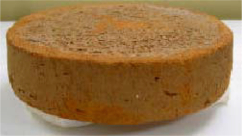
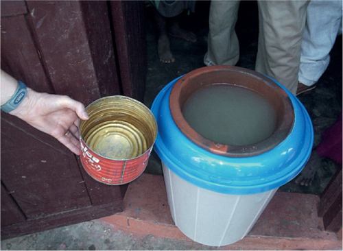
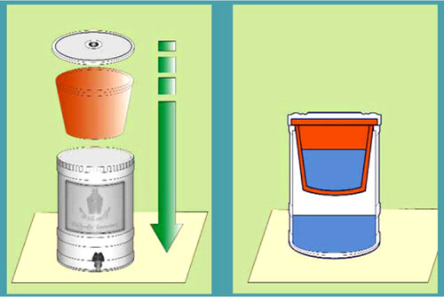
The pot filter was one of the first ceramic filters manufactured by Potters for Peace. A pot filter consists of a ceramic pot perched inside a larger collection bucket. The inner ceramic pot is usually impregnated with colloidal silver for microbial disinfection; the outer collection pot can be plastic. Water is poured into the inner pot, percolates through the bottom of the pot, and is stored in the collection container (see Figures 5.24 and 5.25). The inner pot is fired as one piece, eliminating the possibility of leakage as is seen with use of both the disk filter and the candle filter.
5.2.3.1 Materials, Manufacturing, Removal Efficiency
The inner ceramic pot is manufactured similarly to the disk filters. Clay is mixed with water, rice husks, or sawdust and is formed using a simple hydraulic press. After the pot is fired in an inexpensive kiln, it is either soaked in a solution of colloidal silver for thirty seconds or the colloidal silver solution is painted onto the pot using a brush. If silver is added to the collection system, the amount of biofilm growth can be reduced (Murphy et al., 2009). The pore sizes of the pot filter range from 0.6 to 3.0 μm, which will remove protozoa and bacteria although E. coli will only be erratically removed. Flow rates are slow and range from 1 to 2 L/h. Salsali et al. (2011) reported that the LRV for E. coli was about 2-6 logs and the LRV for protozoa was about 4-6 logs. Removal efficiencies for viruses were less than one log removal.
5.2.3.2 Maintenance
Careful use of the pot filter is required for effective filtration. The inner pot cannot be filled to overflowing because the water could seep through cracks at the very top. According to Resource Development International Cambodia (RDIC), the inside of the pot filter should be cleaned as needed (when the flow decreases substantially), and the storage container should be washed with clean water and soap and air dried in the sun bi-weekly. When performing routine maintenance, the pot filter should not be placed on the ground, hands/tools should be washed before touching any part of the filter apparatus, and the outer edge of the pot filter should not be touched (Murphy et al., 2009). However, field studies have shown that frequent scrubbing and cleaning of the pot have resulted in breakage and failure, reducing the life of the pot filter (Van Halem et al., 2009). A study by Campbell (2005) concluded that pot filters can be used for 2-5 years before they need to be replaced.
5.2.3.3 Cost
• 1 pot filter from Potters for Peace: $9.00 (Dies, 2003)
• Bulk purchase of pot filters from PFP: $6.00 each
• In Cambodia (Van Halem et al., 2009),
• Replacement filters: $2.5-4
5.2.4 Evaluation of Ceramic Water Filters
Ceramic filter systems are low cost and require little maintenance. They can be manufactured locally using local materials. While local manufacturing makes the process more sustainable and helps other people in a developing country make a living, the quality of the products varies, and better quality control is needed. Table 5.2 provides a comparison of the strengths and weakness of using ceramic filters. The average lifetime of these filters is around 1 year, eliminating any long-term applications. According to the Sphere Project (2011), only commercially produced ceramic filters provide the desired flow capacity for emergency survival.
Table 5.2
Strengths and Weaknesses of Ceramic Filters (Dies, 2003)
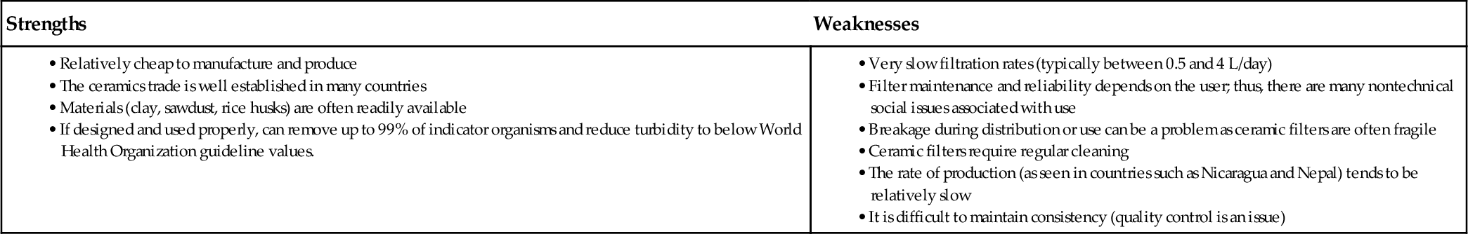
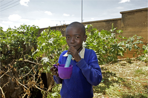
5.2.5 Lifestraw Personal
The Lifestraw Personal is a portable water treatment device that operates using human suction. One end of the microfiltration cartridge is placed in dirty water, and suction is applied to the other end (Figure 5.26). The prefilter at the bottom of the cartridge removes coarse materials larger than 1 mm. The vacuum pressure created from the suction drives the water up through the 0.2 μm pore sizes of the microfiltration membrane at an average flow rate of 200 mL/min (Lifestraw, 2008). The membrane achieves 6 LRV for bacteria and 3 LRV for protozoa. Turbidity is also decreased (Lifestraw, 2008). The device can filter approximately 1000 L of water over its lifetime. To clean the device, blow through the suction end to remove dirty particles from the membrane (Figure 5.27).
5.2.5.1 Cost
• The Lifestraw Personal is available in America for $19.95
• The device is available for humanitarian aid and disaster relief for $6 (Peter-Varbanets et al., 2009)
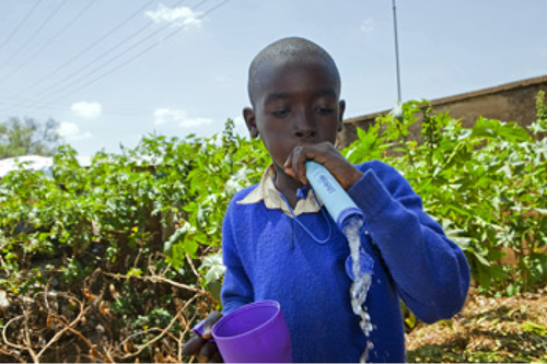
5.2.6 Lifestraw Family
The Lifestraw Family is an ultrafiltration-based system that uses a feed water container elevated above a purification cartridge that contains a hollow fiber membrane (Figure 5.28). The system can last for up to 3 years before needing replacement parts, if properly maintained. Flow rates of 12-15 L/h can be achieved with this device. Source waters that can increase the service life of the device include rivers, wells, and rainwater.
The filter consists of a 2 L feed container with a textile prefilter that removes particles larger than 80 μm. Water flows by gravity through the prefilter, and then small amounts of active chlorine are added to the water to keep the membranes from fouling. Water flows down through the 1 m hose to the ultrafiltration membrane, where the 0.1 bar pressure created by the head allows the water to flow through the 20 nm pores and out the tap; after this point, the water should be properly stored. The 20 nm pore size helps the device achieve a removal value of 6 log reductions for bacteria, 4 log reductions for viruses, 3 log removals for protozoan cysts, and helps decrease turbidity (Lifestraw, 2008). Studies have shown stable operation and high efficiency of bacteria and virus reduction during filtration of 18,000 L of source water (Peter-Varbanets et al., 2009).
A manual backwash is included in the system (the red valve shown in Figure 5.29) and should be run daily to remove all particles that clog the membranes. The prefilter used in the feed container should also be washed daily, while the bucket should be washed weekly. Because of the size constraints of the feed container, constant transport of water and operation of the device is required to provide enough water for consumption.

5.2.6.1 Cost
• This device is not yet available for retail in North America, but the retail price is estimated to be approximately $80 (Amazon.com, 2014).
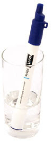
5.2.7 FilterPen
Similar to the Lifestraw Personal, the FilterPen is a product manufactured by Norit that uses human suction power to pull water through microfiltration membranes with pore sizes of 0.2 μm (Figure 5.30). The small pore sizes help the device achieve a removal of a 6 log reductions for bacteria, but the device does not achieve effective removal for viruses. The FilterPen is a disposable device that has a service life of about 1 month. The approximate flow rate is 0.1 L/min. After the membranes become clogged, the filter will not allow any flow through the device, indicating that the device should be discarded. Because this device is so small and light (around 30 g), it can be used by travelers, but it can also be used as an immediate, short-term solution in a disaster.
5.2.7.1 Cost
5.2.8 Chulli (Ovens) Treatment
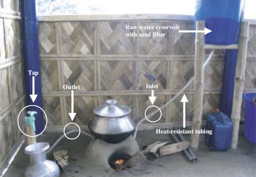
The chulli treatment method uses thermal waste energy to pasteurize water. Chullis are traditional clay ovens used for cooking in areas of rural Bangladesh. These ovens can reach high internal temperatures, but a large portion of the heat is wasted because of inefficiencies. A water purification system has been designed so a hollow aluminum coil is placed inside the oven. One side of the coil is attached to an elevated untreated water supply source (usually a tank). The tank has a clean sand filtration system to reduce turbidity in the water. The other side of the aluminum coil is attached to a tap that opens and closes to allow water to flow through the coil. See Figure 5.31 for an example of the chulli water treatment setup. When the chulli is used for cooking, the tap can be opened to allow hot water to pass through the aluminum coil. Water is collected in a clean bucket once the water flowing out of the tap becomes too hot to touch safely.
When studied in a laboratory setting, the chulli treatment system had a high removal rate of pathogens. It was also hypothesized that the chulli could provide treatment without extra time or fuel (Islam and Johnston, 2006). However, a field study of chullis already in operation found that around 80% of the operators interviewed stopped using their chulli for water treatment because of mechanical breakdowns or complex and inconvenient operation and maintenance (Gupta et al., 2008). Furthermore, studies showed that the pathogen and coliform reductions were not as high in the field as they were in the laboratory (Gupta et al., 2008). While the ovens were cost effective (chulli owners only paid between $1.50 and $6.00 for the equipment), proper use of the ovens required training. When ovens were used incorrectly, the water treatment system did not work, discouraging people from using the system. As this system requires more parts and a complicated setup process, it is not applicable in the acute emergency phase. If chullis already exist in a disaster-affected area, using the chulli water purifier system would provide a more sustainable and long-term response.
5.3 Pressurized Filter Units
Pressurized filtration units are devices that have been designed to produce larger volumes of drinkable water than packaged filtration. These devices can be used by small communities or a group of several families. Energy sources can be solar power, hand power, or gravity. These units produce clean water in amounts that range from enough for one person to enough for communities. Some devices can provide high quality water that is suitable for long-term applications, but these devices typically have a high initial investment. However, because the more expensive devices are able to provide drinking water to large communities for a long time, the cost of water per person per day becomes reasonable. Different types of filtration are used, ranging from microfiltration (MF) to reverse osmosis (RO).
5.3.1 Multistage Backpack Filter
This filtration unit combines three processes: A Pentek polypropylene filter is used to remove any suspended solids, a Pentek carbon block filter removes bad tastes and organics, and a hand-cranked UV disinfection unit from Steripen is used to remove viruses, bacteria, and protozoa (Figure 5.32). The entire system is designed so the unit fits within a backpack and can be easily carried from place to place; see Figure 5.33 (Ray et al., 2012). This system is not yet mass produced, but its applicability for humanitarian aid and disaster relief is being assessed by university researchers in Hawaii and by the Thai military (Ray et al., 2012).


5.3.1.1 Operating Removal Efficiency
The backpack filter system is designed so the unit can be pressurized using a handheld bicycle pump to 7-10 pounds per square inch (psi), or it can operate on gravity using 3 ft of head. The system can efficiently remove coliform bacteria and E. coli and can reduce turbidity. The filters do not remove salts or other dissolved solids. The system works as a batch process and can produce 1 L of water in 5 min; thus, it would work best for individuals or small groups of people. Continuous operation of the system is required because the filtered water has to be disinfected with a hand-cranked UV light. This multiphase unit is designed for a temporary and quick response to disasters and has not yet been tested for long-term applications. The unit fits easily within one backpack and can be carried from site to site, reducing waiting time for clean water during a disaster. The final weight of the backpack and system is about 7 kg. Little maintenance is specified because the filters are not expected to be used for long. Filter service life is also not specified, although the hand-cranked UV lamp was specified for 8000 1-L treatments (Ray et al., 2012).
5.3.1.2 Cost
• Pentek spun polypropylene filter: $3
• Pentek carbon block filter: $10
• Steripen UV disinfection unit: $100
• Total: $113
• Cost of production of a full device is unknown
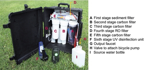
5.3.2 Packaged and Portable RO Filter
The RO system is a six-stage, compact system that is packaged in a Pelican carrying case so it can be easily transported to any fresh source of water (Figure 5.34). The first stage of treatment consists of a polypropylene sediment filter, the second and third stages use carbon block filters to remove odor and organics, the fourth stage uses the RO membrane to remove Giardia cysts and E. coli, the fifth stage uses a polishing carbon block filter, and the sixth stage uses a 1 L hand-cranked UV disinfection Steripen; see Figure 5.35 (Ray et al., 2012). This system is not yet mass produced, but its applicability for humanitarian aid and disaster relief is being assessed by university researchers in Hawaii and by the Thai military (Ray et al., 2012).
5.3.2.1 Operating Removal Efficiency
This RO filter system is designed to operate with two different power sources for flexibility. The system can be operated with a bicycle pump, or it can be pressurized using power from a car battery, which can be charged with a solar panel. Water flows through the first five stages in a continuous process and then is captured at the outlet with the UV unit. It takes the UV unit 1.5 min to disinfect 1 L of filtered water. Removal efficiencies were very high for coliform, E. coli, turbidity, total dissolved solids, and minerals. The system can produce 136-170 L/day, and, if operated continuously for 24 h, can produce 340 L/day. This system is appropriate for a small group or several families. Operation requires supplying the necessary pressure to drive water through the system, batch treating the water with the UV system, and then carefully storing the treated water.
5.3.2.2 Cost
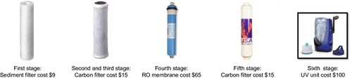
• Osmonics 5-μm rating, Model #1-SED10 polypropylene filter: $9
• KX Extruded 5-μm rating, Model #23-CAB10 carbon block filter: $15
• KX Extruded 5-μm rating, Model #23-CAB10 carbon block filter: $15
• Filmtec 0.0001-μm rating, Model #MEM-45 RO membrane: $65
• Omnipure coconut shell refining carbon 5-μm rating, Model #5-TCR carbon polishing filter: $15
• Steripen UV disinfection unit: $100
• Total: $219
• Cost of production of a full device is unknown
5.3.3 WaterBox
The WaterBox is a packaged solution that uses 10 prefilters and 2 filters that incorporate carbon nanotubes into the media to remove 99.9999% of bacteria, 99.99% of viruses, and 99.9% of cysts from groundwater or fresh surface water (Figure 5.36). The WaterBox can also reduce organics, chemicals, and heavy metals found in polluted water. Water is pumped from a source using a manual bicycle pump or power from an AC/DC source or solar panels. The flow rate of the device is around 2 L/min, and the device has a service life of 30,000 L. Because the device is packaged in a case that is about 2′ × 2′ × 1′, it can be transported directly to water sources and set up within 5 min by an unskilled operator. Hoses and sediment filters must be cleaned periodically to extend the life of the device. Studies were performed on the WaterBox using an independent EPA-certified lab, but no results are available. Because the WaterBox was originally designed for military operations, it may not be available for use in developing countries during emergencies, unless it is donated. This device also produces high quality water rather than a large quantity of water.

5.3.3.1 Cost
• Waterbox sells to military for $7975 (Luquer, 2012)
• Waterbox is offered to humanitarian aid organizations for $3190 (Luquer, 2012)
5.3.4 Lifesaver Jerrycan
The Lifesaver Jerrycan is an ultrafiltration device built into a jerry can. The Jerrycan has an inlet into which water can be poured. The inlet is sealed with a hand pump that is used to pressurize the container. The Jerrycan has a tap at the outlet, preceded by a 15 nm ultrafiltration (UF) filter and an activated carbon filter (Figures 5.37 and 5.38). The 15 nm pore size removes up to 7.5 log reductions of bacteria and 5 log reductions of viruses. Pesticides, heavy metals, and other water pollutants are also reduced. After water is poured into the Jerrycan, the hand pump is used to pressurize the container. The tap can be opened once the container has been pressured enough to release a flow of 2 L/min at 0.1 bar of pressure.


The device can treat up to 15,000 L of water over its lifetime. This can provide a family of four with the minimum amount of water necessary for survival for up to 5 years. The size of the Jerrycan allows storage of up to 18.5 L of treated water. After the filter becomes ineffective, water will not flow through the filter, and the filter should be replaced (Lifesaver, 2011a, b,c). Periodically, the Jerrycan should be rinsed out, and the UF membranes should be unscrewed from the Jerrycan and rinsed in clean water to remove any particulates and to extend the life of the Jerrycan (Lifesaver, 2011a, b,c).
5.3.4.1 Cost
• $270-332 for Lifesaver Jerrycan
• $187-241 for replacement UF filter
5.4 Small-Scale Systems
Areas such as refugee or internally displaced person (IDP) camps that are set up after emergencies need a large amount of clean drinking water. Small-scale systems can meet these large needs as they usually have the capacity for high flow rates or the potential to be scaled up to achieve high flow rates. High-capacity systems are typically commercially produced devices that provide not only a high quantity of flow but also a high quality effluent. Some systems require little maintenance, while other systems may require a great deal of maintenance. These commercial systems require a large amount of initial capital unless they are donated.
For example, Arnal et al. (2001, 2009) discusses a UF system developed for third-world communities (Figure 5.39). This system can use either generators or a manual rotation wheel that produces energy. The capacity of the system can also be increased by adding more ultrafiltration modules. Veolia produces compact skid-mounted systems, not pictured here, that use ultrafiltration membranes; these systems are used during emergencies (Peter-Varbanets et al., 2009).

5.4.1 Sunspring
The Sunspring device is a self-contained, rugged UF unit that can treat groundwater it pumps from wells or from surface water sources. Seventeen of these devices were implemented during the Haiti disaster relief effort and are still supplying water to the communities of Haiti.
The treatment system is made up of a 4.5 gpm pump, a prefilter, a UF system from GE, plumbing, and an automatic backwash that removes impurities (Figure 5.40). The filters are encased within an aluminum cylinder that provides protection. Two solar panels provide power during the day and charge internal batteries, which provide power to treat water during the night. The device is certified by the WQA Gold Seal Program, which means that it removes 99.999% of pathogens from any source water. It can treat 2000-5000 gallons per day, depending on source water conditions and the amount of sunlight. This quantity of water can provide 10,000 people the minimum amount of water needed to survive (2 L/day). The system can be installed within 2-4 h and used almost immediately. The device can last up to 10 years with minimal maintenance. The membranes should not be allowed to dry out or freeze.

The Sunspring comes with a maintenance kit for the required minimal maintenance. Prefilters should be changed weekly to quarterly, depending on the source water quality. Ensuring that the prefilters are clean will help keep the membrane modules clean. Membrane modules need to be changed every 10 years, also depending on the source water quality. In order to test that the Sunspring is effectively removing all pathogens and viruses, membrane integrity testing (MIT) needs to be performed periodically. MIT kits also come with the Sunspring.
5.4.1.1 Cost
The price per Sunspring varies, depending on what is included inside the casing. In the Haiti system, attachments were added to make the system flexible. These attachments included a surface pump for surface water, a submersible pump for wells 30 m deep, and at least a year’s supply of prefilter cartridges. This system costs $25,000. At this price, and assuming the system provides enough water for 10,000 people per day for 10 years, the cost per person per day of these units drops to less than 0.01 dollars per person per day.
• Cost does not include maintenance
5.4.2 Perfector-E
The Perfector-E water purification system from X-Flow (NORIT, the Netherlands) was designed to supply water to tsunami victims in Asia by treating heavily polluted surface water (Figure 5.41). According to manufacturer information (Pentair, 2012), it uses a two-stage pretreatment process consisting of a coarse filter and two parallel microstrainers. The main treatment stage consists of two UF dead-end modules operated with automatic backflushing as well as an optional UV disinfection barrier (Peter-Varbanets et al., 2009). The lifespan of the UF modules ranges from 5 to 7 years, depending on the source water quality. Then the modules should be replaced. The only maintenance that is required is regular cleaning.

The flow rate of this device is around 2000 L/h, and it is powered by a generator that comes with the unit. Perfector-E is able to achieve 99.9999% of bacteria removal and 99.99% of virus removal, even in highly turbid waters. Once set up, the system may be operated by unskilled personnel, and the rugged design allows it to be transported from place to place (PWN Technologies, 2012).
5.4.2.1 Cost
• Approx. $ 26,000 (Peter-Varbanets et al., 2009)
5.4.3 SkyHydrant
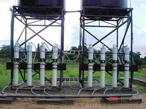
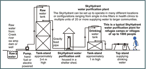
The SkyHydrant is a filtration device that uses UF membrane filtration to treat water for a community. This system can be used individually or in series to increase capacity. One SkyHydrant can produce 500-700 L/h at an operating pressure of approximately 5.7 psi. The SkyHydrant can be used in conjunction with a raw water supply tank that provides the pressure required to power the SkyHydrant. The treated water can be stored in a clean storage tank to provide a continuous supply of treated water; see Figure 5.42 for a drawing of the layout. Communities that already have rooftop water tanks can integrate the SkyHydrant into their piping system (Figure 5.43). This system is complicated to set up as it requires piping, a pump, and storage tanks (Figure 5.43). Thus, the SkyHydrant may be more useful as a long-term, sustained response to a disaster rather than as a short-term solution. The SkyHydrant removes bacteria, viruses, protozoans, and turbidity from source water. Daily cleaning is required to keep the membrane working efficiently although the dirtier the water, the more often the filter will need to be cleaned. According to the operation manual (Skyjuice Foundation, 2010), the UF module does not need to be replaced as long as it is cleaned thoroughly daily. Use of the SkyHydrant is complex so a skilled operator should be designated to manually backwash and clean this system with chemicals periodically (Skyjuice Foundation, 2010).
5.4.3.1 Cost
• SkyHydrant: $1000-2000 per unit
• Does not include costs for infrastructure: a raw water storage tank, a treated water storage tank, and a raw water pump
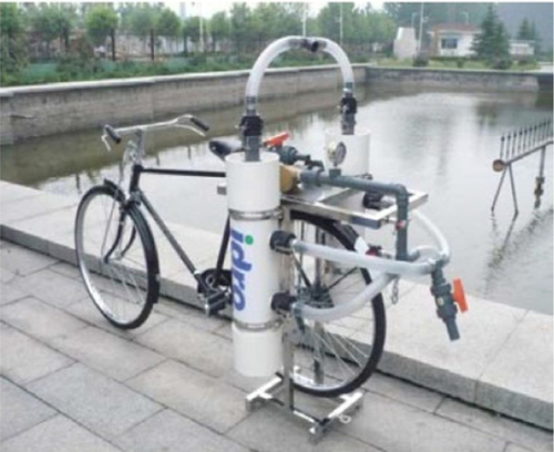
5.4.4 iWater Cycle
In areas where electricity is not available, a bicycle-powered UF membrane system can be used. iWater Cycle has a capacity of 400-900 L/h and can remove turbidity and microbiological contaminants to World Health Organization standards (Figure 5.44). The device is mobile and easy to maintain and operate (Idro, 2010). Maintenance includes manual backwashing when operation pressures exceed normal. This device has been used in Yemen, Myanmar, and Taiwan for emergency relief efforts after the acute emergency phase (Figure 5.45).

5.4.4.1 Cost
5.4.5 Evaluation of Small-Scale Systems
Peter-Varbanets et al. (2009) noted that, “The investment costs of small scale systems are generally too high for communities in developing countries.… These communities also lack trained personnel to maintain these systems and often do not want or cannot assume the responsibility for their performance after their construction by the government or NGOs. The provision of regular maintenance by regional maintenance centers, such as is practiced in some regions in South Africa, needs a certain organization and control and would not be possible in many other countries.”
5.5 Natural Filtration
Natural filtration is a generic term applied to riverbank, lake bank, or SSF. Additionally, desalination of water derived from seashores (beach wells) is considered a natural filtration process. SSF has been described in detail earlier. Here, we will focus on riverbank filtration with some preliminary introduction to lake bank filtration and beach wells for desalination. We will use the generic name “bank filtration” (BF) to represent this natural filtration process.
Bank filtration is a mechanism by which communities located along rivers or lakes develop water supplies from alluvial aquifers using vertical and horizontal (collector type) wells. The sand and gravel deposits comprising these alluvial aquifers yield millions of gallons of fresh water to these communities. When wells are placed sufficiently close to rivers and pumped, river water can be induced to flow to these wells. Bank filtration wells typically produce a larger quantity of water than similarly sized wells that only draw groundwater because the river acts as a steady source. Thus, bank filtration wells have been used by many riverbank communities to augment the groundwater yield that can be expected from an aquifer. The portion of riverbank filtrate in the pumped raw water depends on source water quality, geohydrologic conditions of the aquifer, river-aquifer interface, hydraulic gradient, infiltration rates, hydraulic conductivity, and distance between the riverbank and the pumping wells.
The use of bank filtration for drinkable water dates back more than 100 years. In the lower Rhine region of Germany, riverbank filtration systems have been operating since the 1870s (Schubert, 2002). In the eastern part of Germany, waterworks for the city of Dresden have also operated for more than 100 years (Saloppe since 1875; Tolkewitz since 1898; Hosterwitz since 1908; see Fischer et al., 2006; Ray and Jain, 2011). In the United States, this technology was used initially for industrial water supplies and then for public supplies. The city of Peoria, Illinois, has used bank filtration systems to augment its water supply since the 1940s (Horberg et al., 1950; Schicht, 1965; Marino and Schicht, 1969). Because bank filtration has been shown to be a long-lasting filtration technology, it can be adapted to provide water to affected communities with minimal investment.
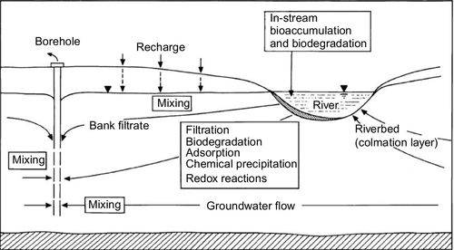
Figure 5.46 shows a diagram of a bank filtration system where a well is located on the bank and the pumping action brings river water to the well. Water from the land side also contributes to the flow to the well. A number of physical, chemical, and biological processes occur as the water moves from the river to the well. Particles that contribute to turbidity are strained out or removed by colloidal filtration (Yao et al., 1971). The temperature of the river water is modulated during its passage through the aquifer. Mixing with groundwater also occurs. Chemical processes such as sorption, ion exchange, biodegradation, geochemical dissolution, and chemical precipitation can occur, depending on the water chemistry and minerals present in the aquifer. Removal of protozoa may occur via straining or colloidal filtration. Bacteria and viruses are primarily removed through colloidal filtration. The redox status of the subsurface affects these chemical and biological processes.
The wells can be either vertical wells or horizontal collector wells. Vertical wells typically have low production rates compared to horizontal collector wells. The preference for a horizontal collector well rather than vertical wells depends on several factors: site hydrogeology, land ownership near the riverbank, and utility preference. In the United States, the preference has been for horizontal collector wells because a large quantity of water can be extracted from one or a few wells. In temperate climates, using a horizontal collector well also reduces the maintenance needs for the well’s pumps and pipes during the winter months as multiple vertical wells will be needed to produce the same amount of water. If the source water is high quality, water produced by BF may not need additional treatment except for chlorination or some other method of disinfection. Horizontal collector wells are often used for pretreatment in the United States. The filtrate passes through the treatment plant; however, chemicals are rarely used for coagulation as the water already has low turbidity.
For emergency water needs, construction of horizontal collector wells may be too expensive. However, vertical wells can be easily sunk along the banks of the rivers or streams. Figure 5.47 shows a series of wells at the Flehe Water Works in Dusseldorf, Germany. These wells are connected by underground siphon systems to a central pumping system. For small systems, wells can be equipped with vertical turbine or submersible pumps.
5.5.1 Design of Wells
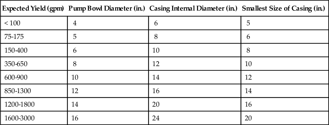
Wells should be designed so that they pump safe and sand-free water for a long time (at least a decade). In unconsolidated formations, gravel may be used in the annular space between the well screens and the formation, depending on the grain size distribution of the natural formation. In some cases, gravel may not be needed if the formation has grains in the appropriate range. Bedrock wells are different from screened wells in an unconsolidated formation. Most bedrock wells are open holes. The diameter of the well has little influence on the specific capacity of the well (Table 5.3). Specific capacity is defined as the well yield per unit of drawdown (Q/s) and is measured in units of gpm per ft of drawdown. Figure 5.48 shows the variation in specific capacity as a function of well radius. Typically, the casing of the well must be at least 2 in. greater than the pump bowl diameter. Two types of pumps can be used in the wells: submersible and vertical turbine pumps.
Table 5.3
Recommended Well Diameters (Driscoll, 1986)
| Expected Yield (gpm) | Pump Bowl Diameter (in.) | Casing Internal Diameter (in.) | Smallest Size of Casing (in.) |
| < 100 | 4 | 6 | 5 |
| 75-175 | 5 | 8 | 6 |
| 150-400 | 6 | 10 | 8 |
| 350-650 | 8 | 12 | 10 |
| 600-900 | 10 | 14 | 12 |
| 850-1300 | 12 | 16 | 14 |
| 1200-1800 | 14 | 20 | 16 |
| 1600-3000 | 16 | 24 | 20 |

These pumps are used within wells if the water table is deeper than the suction lift of centrifugal pumps. Typically, centrifugal pumps are not suitable for wells. Figure 5.49 shows two wells: one with a vertical turbine pump (left) and the other with a submersible pump (right). In the case of a turbine pump, the pump bowl stays in the well (typically above the screen zone), and the motor sits on a pad above the wellhead. The motors for high-capacity wells can be very large (several hundred horse power). Submersible pumps have sealed motor and pump units that are inserted into the well. The power supply cable connects from a power source to the pump. As the diameter of the motor is limited by the diameter of the well, the production capacity of wells equipped with submersible pumps is expected to be less than those of wells equipped with vertical turbine pumps.

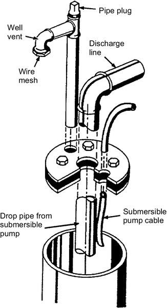
The wells are vented to the atmosphere so that negative pressures do not develop as drawdown occurs in the well. Vent screens prevent foreign objects from entering the wells. The wells need to have a cap or seal to prevent surface water or other contaminants from directly entering the well (see Figure 5.49). Wellheads with turbine and submersible pumps are shown in Figure 5.50. A diagram of a sanitary seal is shown in Figure 5.51.

Wells constructed in unconsolidated (sand and gravel) formations can be either tubular or gravel packed. In a tubular design, the well screen is placed directly against the sand and gravel aquifer. The screen opening is chosen so that it can retain a certain percentage of the aquifer material. Well development, a technique in which the fine particulates from around the screen are removed by water or air or surging1, is conducted to enhance the production capacity of the well and to reduce the potential for clogging. In tubular well design, careful well development is necessary to remove the fine particulates.
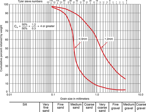
A significant factor in the design of tubular wells is the size of the screen opening (or slot size). The optimum slot size depends on the size distribution of the aquifer material that will stay in contact with the screen. Two important terms are used to define the size distribution of the material: (a) uniformity coefficient (Cu) and (b) effective size (D10). Uniformity coefficient is defined as:

Here “retained size” means the diameter at which a given percentage of the material is retained above the screen. Effective size is 90% of the retained size. A sieve analysis is performed on the aquifer material to obtain this information where the aquifer material is loaded to the top sieve in a nest of sieves of different sizes. Figures 5.52 and 5.53 show sieve analysis data for two different materials—one more homogeneous and the other more heterogeneous. As observed from these figures, the uniformity coefficient for the homogenous material is 2.2 and that for the heterogeneous material is 6. Thus, a homogeneous material will have a size distribution in a narrow band compared to a heterogeneous material. Screen slot size is based on the homogeneity of the aquifer material as well as the stability of the overlying deposits. When the uniformity coefficient is between 3 and 6 (relatively uniform; see Figure 5.52), a screen is selected that retains 40% of the aquifer material if the overlying material is firm (e.g., clay). If the overlying material is subject to caving (such as fine sand), 60% of the aquifer material surrounding the screen must be retained. For heterogeneous aquifer material (Cu ≥ 6), 30% of the material should be retained for a clay-type overburden, or 50% of the material should be retained if the overlying material is subject to caving. In field situations, conditions often do not fit into these categories, thus necessitating some judgment. For example, a screen that retains 40% of the material in a heterogeneous aquifer may be selected if the overlying material is sandy clay with few caving tendencies.


As the aquifer becomes more homogeneous, slot size selection becomes more critical. Small changes in the screen opening result in large variances in the amount of retained material for a homogeneous aquifer because of the steep slope of the particle size distribution graph, as shown in Figure 5.52.
If the aquifer has distinct layers with differing grain size distributions, the slot size of the screens may be tailored to the individual layers. In this case, the 50% size for the finest and the coarsest layers are compared. If the 50% size of the coarsest layer is at least 4 × larger than that of the finest layer (see Figure 5.54), then the screen size should be based on individual layers. If the ratio is less than 4:1, then the screen size should be based on the finest interval in the aquifer. Screen tailoring is not necessary if the total screen length is less than 10 ft. Often, the capacity gained by screen tailoring will not be significant as the well log information may not be sufficiently accurate to warrant changes over short lengths.
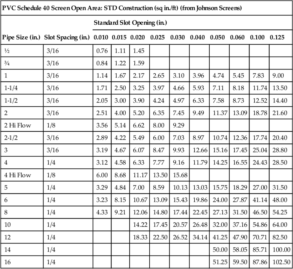
The effective open area of the screen (Ae) is determined using casing diameter and slot size (determined from above) as well as the screen manufacturer’s tables for telescope well screens (see Table 5.4 for data about stainless steel screens and Table 5.5 for data about PVC screens). Because the sand or gravel sits next to the screen openings, a blockage factor of 50% is used when determining Ae.
Table 5.4
Screen Open Areas for Stainless Steel Screens of Different Slot Sizes Typically Used in North America, for Various Diameters of Pipes Large Diameter Free-Flow Screens: Sizes 6P-16T (from Johnson Screens)
| Size (in.) | Max Depth (ft) | OD (in.) | ID (in.) | Weight1 (lb/ft) | Recom. Hang Weight2 (lb) | Collapse Strength1 (PSI) | Intake Area3 (sq in./ft of Screen) | |||||||
| Screen Slot Size (Thousandths of an Inch) | ||||||||||||||
| 10 | 20 | 30 | 40 | 50 | 60 | 80 | 100 | |||||||
| 6P | 100 | 6.5 | 6.0 | 4.4 | 4300 | 87 | 35 | 61 | 82 | 98 | 111 | 123 | 140 | 153 |
| 250 | 6.6 | 6.0 | 4.8 | 4300 | 194 | 20 | 37 | 51 | 64 | 75 | 85 | 102 | 115 | |
| 600 | 6.7 | 5.9 | 6.0 | 8800 | 185 | 20 | 37 | 52 | 65 | 76 | 86 | 103 | 117 | |
| 1000 | 6.8 | 5.9 | 7.6 | 8800 | 677 | 16 | 30 | 43 | 54 | 64 | 73 | 89 | 103 | |
| 8T | 250 | 7.6 | 6.7 | 7.0 | 11,000 | 127 | 23 | 42 | 59 | 73 | 86 | 98 | 117 | 133 |
| 1000 | 7.7 | 6.7 | 8.9 | 11,000 | 468 | 18 | 34 | 48 | 61 | 73 | 83 | 101 | 116 | |
| 8P | 250 | 8.7 | 7.9 | 7.9 | 12,100 | 85 | 26 | 48 | 67 | 84 | 99 | 112 | 134 | 152 |
| 1000 | 8.8 | 7.9 | 10.1 | 20,800 | 314 | 21 | 39 | 55 | 70 | 83 | 95 | 115 | 133 | |
| 10T | 250 | 9.5 | 8.6 | 8.3 | 12,100 | 65 | 28 | 53 | 74 | 92 | 108 | 122 | 146 | 166 |
| 1000 | 9.6 | 8.6 | 10.7 | 12,100 | 242 | 23 | 43 | 60 | 76 | 90 | 103 | 126 | 145 | |
| 10P | 500 | 10.8 | 9.8 | 12.6 | 15,400 | 170 | 25 | 48 | 68 | 86 | 102 | 116 | 142 | 163 |
| 1000 | 10.8 | 9.8 | 17.8 | 15,400 | 226 | 25 | 48 | 68 | 86 | 102 | 116 | 142 | 163 | |
| 12T | 600 | 11.4 | 10.4 | 13.6 | 17,600 | 145 | 27 | 51 | 72 | 90 | 107 | 123 | 149 | 172 |
| 1000 | 11.4 | 10.4 | 19.0 | 17,600 | 192 | 27 | 51 | 72 | 90 | 107 | 123 | 149 | 172 | |
| 12P | 250 | 12.8 | 11.8 | 14.8 | 17,600 | 103 | 30 | 57 | 80 | 102 | 121 | 138 | 168 | 193 |
| 600 | 12.8 | 11.8 | 20.9 | 17,600 | 136 | 30 | 57 | 80 | 102 | 121 | 138 | 168 | 193 | |
| 1000 | 12.9 | 11.8 | 25.2 | 17,600 | 193 | 29 | 55 | 78 | 98 | 117 | 134 | 163 | 188 | |
| 14T | 250 | 12.6 | 11.6 | 13.6 | 14,300 | 108 | 30 | 56 | 79 | 100 | 119 | 136 | 165 | 190 |
| 600 | 12.6 | 11.6 | 19.6 | 14,300 | 143 | 30 | 56 | 79 | 100 | 119 | 136 | 165 | 190 | |
| 1000 | 12.6 | 11.6 | 24.0 | 14,300 | 207 | 28 | 53 | 76 | 96 | 114 | 131 | 160 | 184 | |
| 14P/16T | 250 | 14.1 | 13.1 | 15.5 | 17,100 | 77 | 33 | 63 | 89 | 112 | 133 | 152 | 185 | 213 |
| 600 | 14.1 | 13.1 | 22.2 | 17,100 | 102 | 33 | 63 | 89 | 112 | 133 | 152 | 185 | 213 | |
| 1000 | 14.1 | 13.1 | 27.2 | 17,100 | 148 | 32 | 60 | 85 | 107 | 128 | 146 | 179 | 206 | |
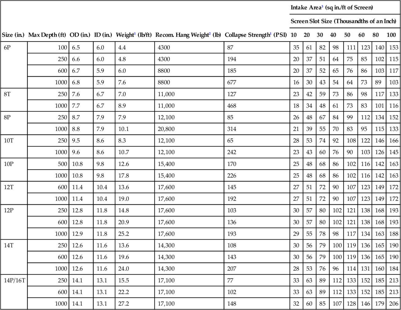
1 Based on 0.030 inch slot size (collapse values contain no safety factor)
2 Recommended hang weight is 50 percent of the calculated tensile strength
3 Transmitting capacity in gpm/ft of screen = open area × 0.31 at 0.1 ft/sec
Table 5.5
Screen Open Areas for PVC Screens of Different Slot Sizes Typically Used in North America, for Various Diameters of Pipes
| PVC Schedule 40 Screen Open Area: STD Construction (sq in./ft) (from Johnson Screens) | |||||||||||
| Pipe Size (in.) | Slot Spacing (in.) | Standard Slot Opening (in.) | |||||||||
| 0.010 | 0.015 | 0.020 | 0.025 | 0.030 | 0.040 | 0.050 | 0.060 | 0.100 | 0.125 | ||
| ½ | 3/16 | 0.76 | 1.11 | 1.45 | |||||||
| ¾ | 3/16 | 0.84 | 1.22 | 1.59 | |||||||
| 1 | 3/16 | 1.14 | 1.67 | 2.17 | 2.65 | 3.10 | 3.96 | 4.74 | 5.45 | 7.83 | 9.00 |
| 1-1/4 | 3/16 | 1.71 | 2.50 | 3.25 | 3.97 | 4.66 | 5.93 | 7.11 | 8.18 | 11.74 | 13.50 |
| 1-1/2 | 3/16 | 2.05 | 3.00 | 3.90 | 4.24 | 4.97 | 6.33 | 7.58 | 8.73 | 12.52 | 14.40 |
| 2 | 3/16 | 2.51 | 4.00 | 5.20 | 6.35 | 7.45 | 9.49 | 11.37 | 13.09 | 18.78 | 21.60 |
| 2 Hi Flow | 1/8 | 3.56 | 5.14 | 6.62 | 8.00 | 9.29 | |||||
| 2-1/2 | 3/16 | 2.89 | 4.22 | 5.49 | 6.00 | 7.03 | 8.97 | 10.74 | 12.36 | 17.74 | 20.40 |
| 3 | 3/16 | 3.19 | 4.67 | 6.07 | 8.47 | 9.93 | 12.66 | 15.16 | 17.45 | 25.04 | 28.80 |
| 4 | 1/4 | 3.12 | 4.58 | 6.33 | 7.77 | 9.16 | 11.79 | 14.25 | 16.55 | 24.43 | 28.50 |
| 4 Hi Flow | 1/8 | 6.00 | 8.68 | 11.17 | 13.50 | 15.68 | |||||
| 5 | 1/4 | 3.29 | 4.84 | 7.00 | 8.59 | 10.13 | 13.03 | 15.75 | 18.29 | 27.00 | 31.50 |
| 6 | 1/4 | 3.23 | 8.15 | 10.67 | 13.09 | 15.43 | 19.86 | 24.00 | 27.87 | 41.14 | 48.00 |
| 8 | 1/4 | 4.33 | 9.21 | 12.06 | 14.80 | 17.44 | 22.45 | 27.13 | 31.50 | 46.50 | 54.25 |
| 10 | 1/4 | 14.22 | 17.45 | 20.57 | 26.48 | 32.00 | 37.16 | 54.86 | 64.00 | ||
| 12 | 1/4 | 18.33 | 22.50 | 26.52 | 34.14 | 41.25 | 47.90 | 70.71 | 82.50 | ||
| 14 | 1/4 | 50.00 | 58.05 | 85.71 | 100.00 | ||||||
| 16 | 1/4 | 51.25 | 59.50 | 87.86 | 102.50 | ||||||
The screen entrance velocity (Vc) is empirically related to aquifer hydraulic conductivity, as shown in Table 5.6. Scientists at the Illinois State Water Survey developed this relationship based on actual case histories of well failures caused by partial clogging of the well walls and screen openings. Unless hydraulic conductivity data exist for a nearby well, one has to estimate the aquifer property. For example, in Illinois, the hydraulic conductivity values for most sand and gravel aquifers range from 700 to 2000 gpd/ft2. From specific capacity data, one can estimate the hydraulic conductivity of the aquifer by conducting a pumping test.
Table 5.6
Optimum Screen Entrance Velocities for Various Hydraulic Conductivity Values of an Aquifer
| Hydraulic Conductivity (gpd/ft2) | Optimum Screen Entrance Velocity (ft/min) |
| > 6000 | 12 |
| 6000 | 11 |
| 5000 | 10 |
| 4000 | 9 |
| 3000 | 8 |
| 2500 | 7 |
| 2000 | 6 |
| 1500 | 5 |
| 1000 | 4 |
| 500 | 3 |
| < 500 | 2 |
Pipe schedules are also standard in North America. Table 5.7 shows the inner diameter, outer diameter, wall thickness, and nominal weights (lb/ft of pipe length) for schedule 40 and 80 pipes. For example, for a 140-in. pipe, the wall thicknesses for 40 and 80 schedule pipes are 0.437 and 0.75 in., respectively.
Table 5.7
Pipe Schedules: Especially Schedules 40 and 80 for Different Diameters
| Schedule 40 and 80 | Schedule 40 | Schedule 80 | |||||
| Pipe Size (in.) | OD (in.) | Avg ID (in.) | Min Wall (in.) | Nom Wt (lb/ft) | Avg ID (in.) | Min Wall (in.) | Nom Wt (lb/ft) |
| 0.50 | 0.840 | 0.608 | 0.109 | 0.161 | 0.528 | 0.147 | 0.202 |
| 0.75 | 1.050 | 0.810 | 0.113 | 0.214 | 0.724 | 0.154 | 0.273 |
| 1.00 | 1.315 | 1.033 | 0.133 | 0.315 | 0.935 | 0.179 | 0.402 |
| 1.25 | 1.660 | 1.364 | 0.140 | 0.426 | 1.256 | 0.191 | 0.554 |
| 1.50 | 1.900 | 1.592 | 0.145 | 0.509 | 1.476 | 0.200 | 0.673 |
| 2.00 | 2.375 | 2.049 | 0.154 | 0.682 | 1.913 | 0.218 | 0.932 |
| 2.50 | 2.875 | 2.445 | 0.203 | 1.076 | 2.289 | 0.276 | 1.419 |
| 3.00 | 3.500 | 3.042 | 0.216 | 1.409 | 2.864 | 0.300 | 1.903 |
| 4.00 | 4.500 | 4.998 | 0.237 | 2.006 | 3.786 | 0.337 | 2.782 |
| 5.00 | 5.563 | 5.017 | 0.258 | 2.726 | 4.767 | 0.375 | 3.867 |
| 6.00 | 6.625 | 6.031 | 0.280 | 3.535 | 5.709 | 0.432 | 5.313 |
| 8.00 | 8.625 | 7.943 | 0.322 | 5.305 | 7.565 | 0.500 | 8.058 |
| 10.00 | 10.750 | 9.976 | 0.365 | 7.532 | 9.492 | 0.593 | 11.956 |
| 12.00 | 12.750 | 11.890 | 0.406 | 9.949 | 11.294 | 0.687 | 16.437 |
| 14.00 | 14.000 | 13.072 | 0.437 | 11.810 | 12.410 | 0.750 | 19.790 |
| 16.00 | 16.000 | 14.940 | 0.500 | 15.416 | 14.214 | 0.843 | 25.430 |

If the hydraulic conductivity data for the wells from pump tests show that a given velocity should be used, but the nearby wells have experienced clogging or chemical encrustation, then a lower entrance velocity may be chosen.
The length of the well screen is determined by the following equation:

where the pumping rate is in gallons per minute, Ae is in ft2/ft of pipe, Vc is the critical entrance velocity in ft/min, and Ls is screen length in ft. Once the screen length has been determined, one should check if this screen length is both realistic and physically feasible. For example, if a 30 ft screen length is needed but only 25 ft of aquifer exist, then the screen length poses a problem. When finer materials exist above or below the aquifer, the screen should be placed at least 1 or 2 ft from the boundary of the aquifer joining these low-permeability layers. A typical design for a tubular screen well is shown in Figure 5.55.
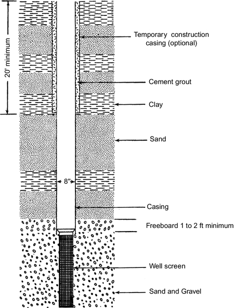
After determining the depth of the top of the well screen, the available drawdown (sa) can be determined. The nonpumping water table (found from other wells or measured) is subtracted from the depth of the top of the screen to find sa. Do not allow the formation to dry out to the screen zone as aeration can promote metal precipitation and encrustation. From the specific capacity data for the well, the maximum pumping rate can be determined. The specific capacity is estimated by comparing the Q/s of nearby wells. A theoretical specific capacity for a new well can be estimated from the following equation:
where: Q/s = specific capacity, in gpm/ft; Q = discharge, in gpm; s = drawdown, in ft; T = transmissivity, in gpd/ft; S = coefficient of storage; rw = nominal radius of the well, in ft; t = time after pumping began, in min.
Because conditions rarely lend themselves to just one design option, an alternative design should be evaluated for comparison. This is especially important in cases in which both a natural backfill and artificial (gravel) pack are possible. While in the past both uniform and graded gravel packs were used, these days only uniform gravel packs are used. In general, a gravel pack is needed if the effective size of the aquifer material is less than 0.01 in. and Cu is less than 3.
The ideal size of the gravel pack is based on the 50% size of the finest interval of sand and gravel that needs to be retained by the pack. This includes units of sand and gravel or other unstable formations that the gravel pack contacts, even though they are at a level at the top of the screen. If the exact sizes of these materials are not known, but there are indications that they are fine grained, care should be taken to segregate these fine materials from the gravel pack.
The 50% size of the formation is multiplied by 3 to obtain the 95% retained size of the pack and multiplied by 5 to obtain the 5% retained size. The particle size data for a commercially available gravel pack material (from Northern Gravel Company, Muscatine, IA) is shown in Figure 5.56 and Tables 5.8 and 5.9.
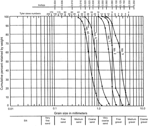
Table 5.8
Approximate Size Ranges of Well Gravel Pack Material from Northern Gravel Company
| No. | Size Range (in.) | Size Range (mm) |
| 00 | 0.017-0.038 | 0.42-0.99 |
| 0 | 0.023-0.060 | 0.59-1.6 |
| 1 | 0.049-0.090 | 1.2-2.2 |
| 2 | 0.064-0.125 | 1.6-3.2 |
| 3 | 0.075-0.180 | 1.8-4.6 |
Table 5.9
Continuous Screen Slot Sizes Acceptable for Use with Well Gravel Pack Material from Northern Gravel Company, Muscatine, IA
| No. | Slot Size |
| 00 | 18 |
| 0 | 25 |
| 1 | 55 |
| 2 | 65 |
| 3 | 80 |
The slot size of the gravel packed well is selected so that it retains 90-95% of the gravel. The screen effective open area is determined same way, applying a blockage factor of 50%. The screen entrance velocity is also determined based on the average of the formation and the gravel pack hydraulic conductivities. Most uniform gravel pack materials have higher conductivities (> 6000 gpd/ft2, which is at the top of the Table 5.6), which means that, for the smallest possible hydraulic conductivity (K) of the formation, the corresponding entrance velocity for a gravel packed well built in this formation will be 8 ft/min. Based on experience, if the formation has a K value less than 2000 gpd/ft2, a safer and more realistic Vc can be obtained by doubling the formation’s K value. The well screen length is based on the equation presented earlier.
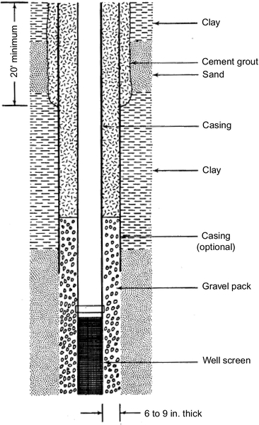
The thickness of the gravel pack can vary. However, a too thick pack interferes with the development of the well and makes the well less efficient. Use of a pack that is too thick may result in the screen being exposed to the formation material, which causes sand pumping. Based on experience, the gravel envelope should be between 6 and 9 in. Thus, the borehole must be the casing diameter plus 12-18 in.
The filling depth of the gravel in the annulus (the space between the formation and the casing/screen) depends on the characteristics of the unconsolidated materials between the land surface and the well screen. The gravel pack is generally taken some distance above the screen to ensure the screen is not exposed to natural formation (especially of gravel settling during well development). Generally, 20-25 ft of gravel is needed above the screen. If the gravel comes in contact with materials that are smaller than the diameter of the formation material for which the gravel pack was selected, fine particulates can migrate through the gravel to the well screen. In such cases, the gravel pack must be terminated before reaching the fine materials and sealed with bentonite or cement (see Figure 5.57).
After the pack design is complete, the results must be checked against the physical realities of tubular wells, as discussed previously. The approximate available drawdown should be determined and a maximum drawdown estimated to check if the design is reasonable and realistic under the existing conditions. Often, conditions are encountered where both gravel-packed and tubular designs are possible. In that case, cost must be weighed to determine the final design.
The other type of well that is often used for water supplies is bedrock wells. These wells are constructed in fractured bedrock where the casing is generally installed 50 or 100 ft below the water table. An open hole, which contains the pump, is present below this level. However, such wells are not typically used in bank filtration systems.
Once a well is installed, development of the well must be done to remove the fine particulates and to enhance the specific capacity. This, in turn, increases the economic life of the well. Typical development procedures include pumping, surging, use of compressed air, hydraulic jetting, use of explosives, and hydraulic fracturing (for bedrock wells). Pumping and surging seem to be the most common techniques used in less developed areas. A well is pumped in a series of steps, and discharge is produced ranging from low discharge to a discharge greater than the design capacity. The intake of the pump is lowered to the middle of the screen zone to remove the most fine particulates. At each step, the water is pumped until it runs clear, and then the discharge rate is increased to the next higher level. This irregular and noncontinuous pumping agitates the fine material around the screen. Coarser materials that fall into the well are removed by a bailer. Development by pumping is invariably the final procedure if other techniques are used.
Surging is another method used for developing water wells. A surge block is attached to a drill stem and moved up and down in a reciprocating motion (Figure 5.58). The gap between the well screen and the surge block is typically 2-5 cm. As the block is moved up and down, the water from the well is pushed into the formation via the gravel pack and then sucked back into the well bringing with it the fine particulates. Pushing the water into the formation may also break up any particle bridging. At the end, the collected fine particulates in the well are bailed out. Finally, a pumping procedure cleans up the fine particulates. Often, chemicals, particularly sodium hexametaphosphate (typically used to disperse clay), may be used in addition to surging.
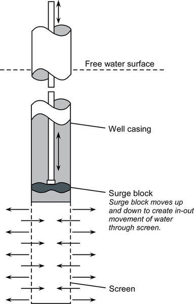
After the well is developed and the pump is installed, a chlorination system is installed. Various chlorination systems are discussed in Sections 4.3 and 4.4. After the chlorination system is installed, the water quality should be tested and then supplied to the affected population.
If a large quantity of water is needed, multiple wells could be drilled on the bank of a river, and the pumped water from each well could be routed through one discharge pipe. In some riparian locations, where the depth of the surface to groundwater is relatively shallow (within the suction lift of a pump), a series of filter screens can be inserted and a centralized caisson can be used for pumping. For example, the Dusseldorf Water Works has a series of such filter screens, which have siphon tubes connected to a central pumping caisson (Figure 5.59).
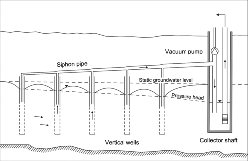
Natural filtration has numerous advantages over the use of surface waters (Ray et al., 2002a). The pumped water from BF wells may not require any additional treatment besides disinfection. Even if a community rebuilds its water treatment plant after a disaster, conversion of a surface water intake system to a bank filtration system may reduce the costs associated with water treatment and remove a variety of contaminants that adversely affect water quality. As the particles are relatively low in count, need for coagulation and flocculation is reduced. Removal of natural organic matter also reduces the potential formation of trihalomethane in drinking water after chlorination. However, if the water contains significant amounts of dissolved iron or manganese, aeration may be needed to remove them. In addition, mineral removal depends on the hardness of the BF water.
Turbidity reduction through BF wells is sufficient to meet the drinking water standards in most locations without additional treatment. Figure 5.60 shows the turbidity of filtrate at Collector Well #1 of the Sonoma County Water Agency (SCWA) in Santa Rosa, California. The turbidity of the Russian River reached almost 500 NTU in the winter and early spring in both 2005 and 2006. During those periods, the filtrate from Collector Well #1 was still under 0.3 NTU. Figure 5.61 shows the river turbidity as well as the turbidity of filtration from the first well of the Louisville Water Company (LWC) in Louisville, Kentucky, in 2000. The river turbidity exceeded 800 NTU at some time during the monitoring period. However, the turbidity of the filtrate was around 0.2 NTU most of the time. Like the SCWA results, the LWC study showed that the spikes of turbidity in the river were not reflected in the filtrate from the wells.
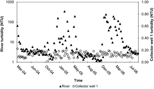
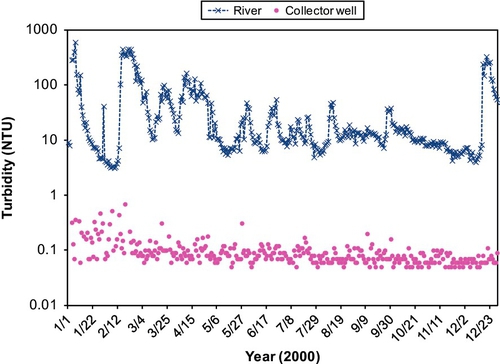
The passage of river water through a BF well also helps stabilize the temperature of the filtrate. Figure 5.62 shows the variation in the temperature of the river water as well as the filtrate from the first collector well. This figure shows that the water temperature of the Ohio River varied between 2 and 33 °C while the filtrate temperature varied between 12 and 25 °C. There is a time lag between the high and low temperature values of the surface water and filtrate. These are shown by the dotted lines on Figure 5.62; which vary between 4 and 6 weeks. The viscosity of river water in winter months can be twice as high as it is in summer, which has several effects. First, well yield will decrease as the apparent hydraulic conductivity is reduced. However, in winter, the demand for water is usually low so this effect would not have any negative consequences. Second, if the surface water is used in a treatment plant, the temperature variation of the water would require the operator to adjust coagulant dosing and other unit operations that are affected by temperature. The moderation of water temperature through bank filtration reduces these difficulties.
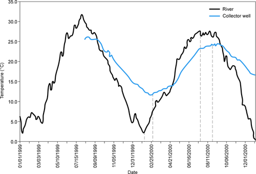
Predicting the temperature of water in bank filtrate is important to control processing and simulate chemical reactions because biogeochemical reactions are temperature sensitive. For example, degradation of dissolved organic carbon depends on temperature. The Dusseldorf Water Works in Dusseldorf, Germany, uses bank filtration to supply water to the city’s residents. Figure 5.63a shows an aerial view of the river with the treatment plant on one side. Because the plant is on a bend, the bank closest to the treatment plant is steep, and it receives more sediments than the opposite bank, which causes clogging. Figure 5.63b shows a cross-section of the river near the treatment plant. Three monitoring wells are positioned near the production well. Well C is located 50 m away on the land side of the production well. Wells A and B are between the production well and the river. Each of these monitoring wells has the ability to sample water at different depths. (In the figure, the monitoring ports are marked 1 through 6, depending on the well.) The aquifer is layered at this site with hydraulic conductivity values ranging from 3.01 × 10− 3 to 6.37 × 10− 3 m/s from top to bottom. At the river-aquifer interface, there is a clogging layer with a hydraulic conductivity of 1.04 × 10− 6 m/s near the bank and 9.26 × 10− 4 m/s near the mid-section of the river.

Sharma et al. (2012) conducted a simulation of the temperature in the bank filtrate using heat as a reactive species in the multi-species transport model used. Figure 5.64 shows the temperature of the river water during a period of more than 1 year and the corresponding measured and simulated temperature values in port 1 of monitoring well B. As shown in this figure, the peak temperature in port 1 of this well was close to 10 °C cooler in summer, and the peak temperature of the bank filtrate was reached approximately 2 months after the peak temperature of the surface water was reached. The simulated and measured values are consistent.

Sharma et al. also conducted a simulation of the impact variable temperatures had on the concentration of oxygen in bank filtrate. In most isothermal models, the temperature is assumed to be a fixed number. Sharma et al. found that, by assuming a fixed temperature in the simulation domain (5, 15, or 25 °C), they were not able to match simulated oxygen concentrations to the observed concentration values at port 1 of monitoring well B (Figure 5.65). In this figure, the blue dotted line shows the temperature of the river water over time. At an assumed 15 °C, the researchers’ match was good between days 300 and 450; however, the fit was poor in the early part of the simulation. This figure also shows that for 100 days (between days 250 and 350), the bank filtrate nearly became anoxic.
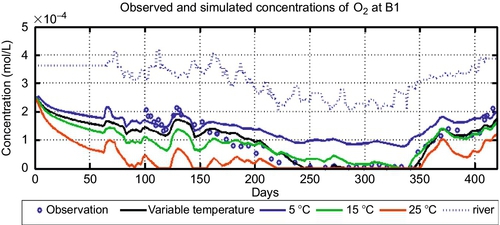
In Figure 5.66, Sharma et al. show the difference in concentrations of oxygen, dissolved organic carbon, sulfate, and nitrate by assuming temperature-controlled degradation of dissolved organic carbon (DOC) and other reactions involving oxygen, nitrate, and sulfate. They also conducted simulations without considering the effect of DOC degradation and temperature variations. The open circles are observed values, the red lines are values with reactions, the green lines are values without reactions, and the blue lines are the values in the river water. We find that if we do not include temperature-controlled reactions for DOC degradation, the predicted oxygen concentration in bank filtrate does not match observed values. However, as shown in Figure 5.64 as well as in the top right panel of Figure 5.65, if we do include temperature-controlled reactions, we see a good match between the observed and simulated values. In the lower right panel of Figure 5.65, we also see nitrate is substantially reduced during the period when oxygen is depleted. For sulfate (the lower left panel), a simulation with reactions was not any different from the one without reactions as the system did not reach a sulfate-reducing condition. In the top left panel, the measured and simulated DOC show that about 1 mg/L is nonbiodegradable. As the river water enters the aquifer, the biodegradable portion of DOC is consumed by bacteria through aerobic respiration. A simultaneous decrease in oxygen occurs. As the oxygen is depleted between days 250 and 350, nitrate is used as an electron acceptor. As the nitrate is not fully removed, other redox reactions such as iron reduction or sulfate reduction do not occur. Thus, it is important that utility managers have an understanding of the effect of the redox conditions on resulting water quality.
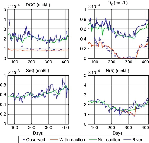
Bank filtration systems also have other benefits. The formation of disinfection byproducts (DBPs) is an issue for water utilities that treat surface water with chlorine. The TOC in the river water is considered an indicator of the formation potential of DBPs. Bank filtration removes a portion of the TOC during the water’s passage through the soil. At LWC, experiments were conducted at the first collector well to observe the amount of TOC removal when flow distance from the river-aquifer interface was increased. The collector well had seven laterals and four of them were directed toward the river (Figure 5.67). Lateral 4, which was directed toward the river and had a depth of 50 ft (15 m), was monitored, and piezometers were installed at depths of 0.6 m (W1), 1.5 m (W2), and 3 m (W3).
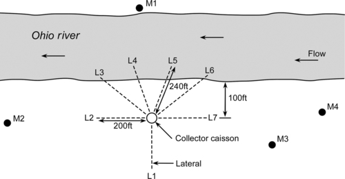
Figure 5.68 shows that the TOC concentration in the river varied from about 1.7-3.8 mg/L, with the peak occurring the late fall. Piezometers W1, W2, and W3 showed similar removal efficiencies, implying that a substantial amount of removal occurred in the first 0.6 m because of microbial reactions. The concentration of TOC in Lateral 4 was somewhat lower than that found at piezometer W3; this could be because of (a) additional degradation of TOC during the water’s passage through the aquifer, or (b) dilution with background groundwater. Typically, groundwater has a lower TOC than river water. Figure 5.69 shows the percentage of TOC reduction at the piezometers as well as Laterals 1, 2, and 4.
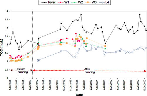

TOC removal at W1 (0.6 m) was about 30%, and this value did not significantly change until the depth of 3 m. However, TOC from Lateral 4, which was about 15 m below the riverbed, had a TOC that was 50% lower than that of the river water. As stated earlier, this could have been because of degradation of TOC or dilution with background groundwater. Lateral 1 extended away from the river and primarily pumped ground water. Its TOC was about one-third of that in the river. Lateral 2 received part groundwater and part river water.
Wang (2002) conducted formation potential tests for trihalomethanes, haloacetic acids (six of them), and total organic halogens on the water samples collected from the three piezometers (W1, W2, and W3) and Lateral 4 (Figure 5.70). The formation potentials were reduced between 25% and 50% in the waters from the piezometers and between 40% and 60% at Lateral 4. These values indicate TOC removal at these locations.

Figure 5.71 shows the log removal of total coliforms at LWC’s collector well. The level of log removal varied from a low of 1 (90%) to a high of 5 (99.999%). Lower removals are typically associated with high flow events in rivers when the protective sediment at the river-aquifer interface gets washed away. Figure 5.72 shows the removal of spores of B. subtilis at Laterals 1, 2, and 4 as well as the collector well. The river water had about 10,000 spores per 100 mL. Figure 5.73 shows the log removal values of these spores at L4 as well at the three piezometers (W1, W2, and W3). Between W1 and L4, the removals were between 1.5 and 3.5 log values.
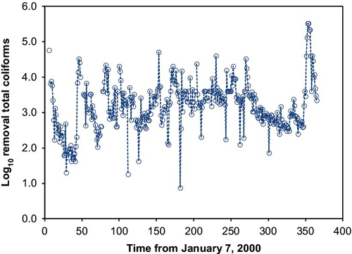


Removal of microorganisms or other contaminants in river water can be low in collector wells compared to vertical wells in bank filtration systems. Typically, collector wells are built very close to a river, and they are pumped at rates much higher than vertical wells. As a result, the flow distance of the water is short. Removal rates for microbes can be much higher for vertical wells, which are typically pumped at lower rates and are built some distance away from the river. Therefore, the wells implemented in emergency scenarios should be vertical wells because they remove more pathogens and other chemicals.
Schijven et al. (1999) examined the removal of colliphages MS-2 and PRD1 in riverbank filtration wells (vertical wells) located in the lower Rhine Valley in the Netherlands. As the well distance increased from the river, so did the travel time of the water. These researchers observed an increase of more than 8 log removal values as the water’s travel time increased to about 25 days (Figure 5.74). Medema et al. (2000) examined the removal of total coliforms and colliphages at a dune recharge site in the lower Rhine Valley in the Netherlands. They observed 4-6 log removals, depending on the organism (Figure 5.75).
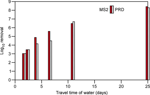

Ray et al. (2002a) studied the removal of the pesticide atrazine at a collector well on the bank of the Illinois River that draws water for the city of Jacksonville, Illinois. Most of the time, the concentration of atrazine in the well was below detection, and the level in the river varied between 1 and 4 mg/L. In a flood event in the spring of 1996, the concentration of atrazine in the river water increased to about 11 mg/L (Figure 5.76). However, there was a small breakthrough in the well, and the concentration in the well increased to about 1.1 mg/L (about 90% removal). The current maximum contaminant limit (MCL) for atrazine is 3 mg/L. In essence, no additional treatment was required to remove the atrazine.

Schubert (2002) monitored levels of the complexing agent EDTA and the drug diclofenac at the bank filtration site in Dusseldorf. EDTA in the surface water varied between 6 and 12 μg/L (Figure 5.77) and that in the bank filtrate between 2 and 3 mg/L. The antibiotic diclofenac in the river water varied from 0 to 500 ng/L (Figure 5.78). Most of the time, the filtrate contained no diclofenac. However, in one incidence (during the peak event of the river), the concentration in the filtrate was about 40 ng/L.
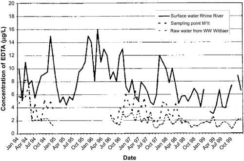
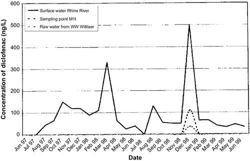
It is clear that BF removes a variety of pollutants present in surface water. For proper operation of BF wells, it is essential that the river or stream has a high, but nonscouring, flow rate and clogging is minimal. Bank filtration systems located on the banks of stagnant rivers, such as those behind dams or diversion structures, seem to experience some water quality issues caused by deposition of organics (such as algae) on the riverbed. This leads to quick depletion of oxygen. In such cases, iron and manganese become soluble. Siting of the wells is also important from the water production perspective because a higher yield is possible when wells are located inside a river bend rather than on the outside (Figure 5.79). Figure 5.80 shows the flow path of water coming to a bank filtration well along the Elbe River. It seems most of the water comes from the other side of the river. In this particular case, the high nitrate level detected in the well was caused by water flowing from grape growing areas on the other side of the river even though the river nitrate level was lower than that of the pumping well.
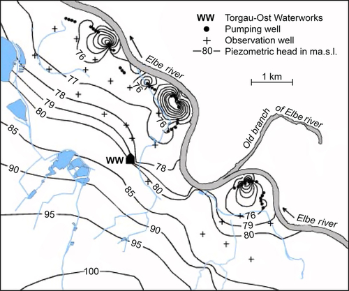
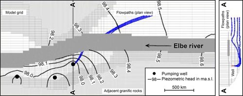
In developing countries, the use of natural filtration has significant potential where the budget for building and maintaining water treatment plants may not be able to keep up with population growth. Even if bank filtration is used only for pretreatment, the resulting water quality will be far superior to that of the surface water. Natural filtration can also defer expansion costs of water treatment plants. Appropriate technologies can be adapted to local situations to make bank filtration systems work. For example, Koop wells used in the hilly state of Uttarakhand where filter and a piece of geotextile are used to wrap the screened pipes, to produce filtrate (Sandhu et al., 2011). This also increases the travel time of the water from about 5 min to more than 4 h. In field settings, the placement of wells and pumps should be optimized so that the travel time is not too short to reduce the contaminants in the river water.
Developing countries such as China, Egypt, and India face tremendous challenges in keeping their rivers clean because of industrial discharge. In such situations (where the source water is poor quality), the bank filtrate probably cannot be supplied to consumers without additional treatment. Many water treatment plants in these countries pretreat water with chlorine to get rid of color and then disinfect to maintain chlorine residuals in the system. Rarely reported or recognized, however, is the positive effect BF has on minimizing the formation of carcinogenic disinfection byproducts.
Ray (2008) summarized the worldwide potential of riverbank filtration: Vast areas of the world (Asia, Africa, and South America) are still untapped territories in which to build bank filtration systems. However, Sandhu et al. (2011) highlight challenges that a bank filtration system can face in a developing country such as India. Bank filtration is rapidly expanding in South Korea, where the technology has been found to be an inexpensive alternative to the membrane treatment process.
The potential climate change effects on bank filtration should also be examined. As the climate becomes more erratic (warmer summers or colder winters) and low-flow periods in river systems become prolonged, the impact of waste discharge to rivers can adversely affect the operation of bank filtration systems. Schoenheinz and Grischek (2010) have pointed out the potential climate change effects on bank filtration. Eckert et al. (2008) highlight the impact of climate-induced low flows in the Rhine River as well as the impact of warm water temperatures on the development of anoxic conditions at Dusseldorf’s bank filtration facility.
Floods generated by heavy rainfalls can cause a lot of diffuse pollutants to enter rivers in agricultural watersheds, especially in spring when snow is also melting. Bacteria, pesticides, synthetic and dissolved organics, and nutrients are the primary contaminants during this time. In flood situations, finding supplies of electric power as well as preventing pump motors from being submerged can be issues for bank filtration systems. Thus, it is advisable to build a well house on high ground and put berms of embankments around a chlorine contactor.