
Chapter 14: Interpretable semisupervised classifier for predicting cancer stages
Isel Graua; Dipankar Senguptaa,b; Ann Nowea a Artificial Intelligence Lab, Free University of Brussels (VUB), Brussels, Belgium
b PGJCCR, Queens University Belfast, Belfast, United Kingdom
Abstract
Machine learning techniques in medicine have been at the forefront addressing challenges such as diagnosis, prognosis prediction, or precision medicine. In this field, the data are sometimes abundant but comes from different data sources or lack assigned labels. The process of manually labeling these data when conforming to a curated dataset for supervised classification can be costly. Semisupervised classification offers a wide range of methods for leveraging unlabeled data when learning prediction models. However, these classifiers are commonly deep or ensemble learning structures that often result in black boxes. The requirement of interpretable models for medical settings led us to propose the self-labeling gray box classifier, which outperforms other semisupervised classifiers on benchmarking datasets while providing interpretability. In this chapter, we illustrate the applications of the self-labeling gray box on the omics and clinical datasets from the cancer genome atlas. We show that the self-labeling gray box is accurate in predicting cancer stages of rare cancers by leveraging the unlabeled instances from more common cancer types. We discuss insights, the features influencing prediction, and a global representation of the knowledge through decision trees or rule lists, which can aid clinicians and researchers.
Keywords
Cancer stage prediction; Explainable artificial intelligence; Semisupervised classifier; Self-labeling; Gray box model
Acknowledgments
This work was supported by the Flemish Government (AI Research Program); the IMAGica project, financed by the Interdisciplinary Research Programs and Platforms (IRP) funds of the Vrije Universiteit Brussel; and the BRIGHT analysis project, funded by the European Regional Development Fund (ERDF) and the Brussels-Capital Region as part of the 2014–20 operational program through the F11-08 project ICITY-RDI.BRU (icity.brussels).
1: Introduction
Cancer is a disease or group of diseases caused by the transformation of normal cells into tumor cells characterized by their uncontrolled growth. This is a multistage process, triggered and regulated by complex and heterogeneous biological causes (Hausman, 2019). In the process, there is a gradual invasion and destruction of healthy cells, tissues, and organs by the cancerous cells (Hausman, 2019). Therefore, a key factor in the diagnosis of cancer is identifying the extent it has spread across the body: stage and TNM grade (tumor, node, metastasis) (Gress et al., 2017). This is also important for treatment planning and patient prognosis. Clinically, the cancer stage describes the size of the tumor and how far it has spread in the body, whereas the grade of a cancer describes its growth rate, i.e., how rapidly it is spreading in the body. Usually, an initial clinical staging is made based on the laboratory (blood, histology, risk factors) and imaging (X-ray, CT scans, MRI) tests, while a more accurate pathological staging is usually performed postsurgery or via biopsy.
Clinical advancements including computational approaches based on machine learning have been developed since the 1980s, which can be used for cancer detection, classification, diagnosis, and prognosis (Cruz and Wishart, 2006; Kourou et al., 2015). With the advancement of omics-based technologies and availability of the omics data (e.g., genome, exome, proteome, etc.) along with the clinical data, there have been impeccable improvements in these methods (Zhang et al., 2015; Zhu et al., 2020). However, mostly these developments have been for common cancer types (colon, breast, prostate, etc.), like the prostrate pathological stage predictor based on biopsy patterns, PSA (prostate-specific antigen) level, and other clinical factors (Cosma et al., 2016). In similar terms, there are staging predictors available for breast and colon cancer based on clinical factors (Said et al., 2018; Taniguchi et al., 2019). There are more than 200 types of cancer developing from different types of cells in the body; lung cancer being the most common (11.6% of total cases, 18.4% of total cancer-related deaths), followed by breast, colorectal, and prostate cancer (Bray et al., 2018; WHO, 2020). However, 27% of the cancer types, like bladder cancer, melanoma, are less common, whereas 20% of them, like thyroid cancer, acute lymphoblastic leukemia, are rare or very rare (Macmillan Cancer Support, 2020; Cancer Research UK, 2020). A major challenge with such rare cancer types is the availability of data, as they have an incidence rate of 6:100,000. The prediction performance of machine learning approaches for classification, diagnosis, prognosis, etc., involving rare cancers is thus limited by the lack of labeled data.
Semisupervised classification (SSC) constitutes an alternative approach for building prediction models in settings where labeled data are limited. The general aim of SSC is improving the generalization ability of the predictor compared to learn a supervised model using labeled data alone. The main assumption of SCC is that the underlying marginal distribution of instances over the feature space provides information on the joint distribution of instances and their class label, from where the labeled instances were sampled. When this condition is met, it is possible to use the unlabeled data for gaining information about the distribution of instances and therefore also the joint distribution of instances and labels (Zhu et al., 2020). SSC methods available in the literature are based on different views of this assumption. For example, graph-based methods (Blum and Chawla, 2001) assume label smoothness in clusters of instances, i.e., two similar instances will share their label, therefore an unlabeled instance can take the label of its neighbors and propagate this label to other neighboring instances. Semisupervised support vector machines (Joachims, 1999) assume that the boundaries should be placed on low-density areas, which is complementary to the cluster view described earlier. In this method, unlabeled instances help compute better margins for placing the boundaries. Generative mixture models (Goldberg et al., 2009) try to find a mixture of distributions (e.g., Gaussian distributions), where each distribution represents a class label. They learn the joint probability by assuming a type of distribution and adjusting its parameters using information from the labeled and the unlabeled data together. Finally, self-labeling methods use an ensemble of classifiers trained on the available labeled data for assigning labels to the unlabeled instances, assuming their classifications are correct. This assumption makes self-labeling the simplest and most versatile family of semisupervised classifiers, since they can be used with practically any base supervised classifier (Van Engelen and Hoos, 2020). Although SSC methods achieve very attractive performance in terms of accuracy in a wide variety of problems (Triguero et al., 2015), they often result in complex structures which lead to black boxes in terms of interpretability.
Nowadays, an increasing requirement in the application of machine learning is to obtain not only precise models but also interpretable ones. Interpretability is a fundamental tool for gaining insights into how an algorithm produces a particular outcome and attaining the trust of end users. Although several formalizations exist (Barredo Arrieta et al., 2020; Doshi-Velez and Kim, 2017; Lipton, 2016), interpretability is directly connected to the transparency of the machine models obtained. The transparency spectrum (see Fig. 1) starts from completely black box models which involve deep or ensemble structures that cannot be decomposed and mapped to the problem domain. While on the opposite extreme are the white box models which are built based on laws and principles of the problem domain. This side also includes those models which are built from data, but their structure allows for interpretation, since pure white boxes rarely exist (Nelles, 2001).
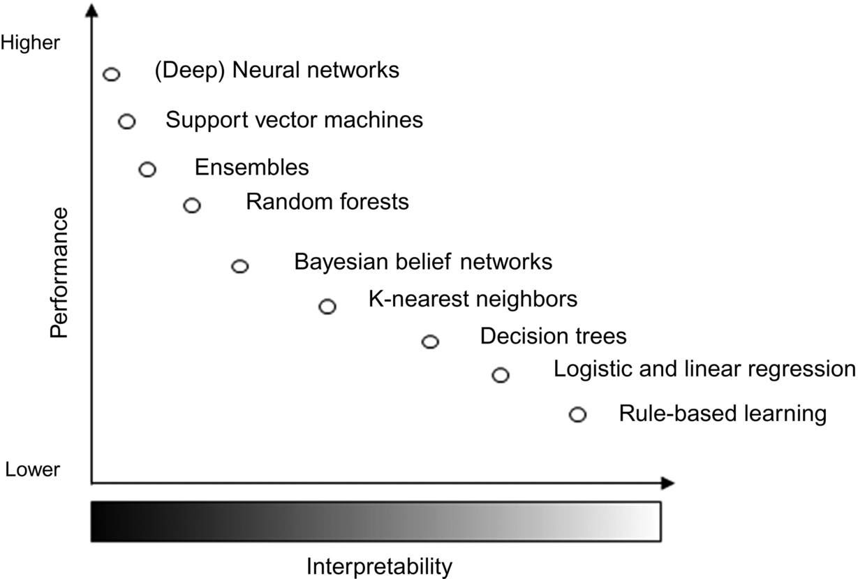
White box techniques are commonly referred as intrinsically interpretable and vary in the types of interpretations they can provide as well as their limitations for prediction. Examples of intrinsic interpretable methods are linear and logistic regression (Hastie et al., 2008), k-nearest neighbors, naïve Bayes (Altman, 1992), decision trees (Quinlan, 1993), and decision lists (Cohen, 1995; Frank and Witten, 1998). On the opposite side, black boxes are normally more accurate techniques that learn exclusively from data, but they are not easily understandable at a global level. As a solution, there exist several model-agnostic post hoc methods for generating explanations which quantify the feature attribution in the prediction of certain outcomes according to the black box. Some examples of these techniques are dependency plots (Friedman, 2001), feature importance metrics (Breiman, 2001), local surrogates (LIME) (Ribeiro et al., 2016), or Shapley values (Lundberg and Lee, 2017; Shapley, 1953). While explanations provided by intrinsically interpretable models are derived from their structure and easily mappable to the problem domain, model-agnostic ones are often local or limited to feature attribution rather than a holistic view of the model.
Global surrogates or gray box models take the best of both worlds while trying to find a suitable trade-off between accuracy and interpretability. The idea behind this technique is to distill the knowledge of a previously trained black box model in an intrinsically interpretable one. In this way, the prediction capabilities are kept to some extent by the black box component, while the white box learns to mimic these predictions through a more transparent structure. In our earlier work (Grau et al., 2018, 2020a), we proposed a gray box model for SSC settings, called self-labeling gray box (SLGB). Our method uses the self-labeling strategy from SSC for assigning a label to unlabeled instances. This part of the learning process is carried out by the more accurate black box component. Once all instances have been self-labeled, then a white box model is learned from the enlarged dataset. The white box component, being an intrinsically interpretable classifier, allows for interpretable representation of the model at a global level as well as individual explanations for the prediction of instances. The SLGB outperforms several state-of-the-art SSC algorithms in a wide benchmark of structured classification problems where labeled instances are scarce (Grau et al., 2020b).
In this chapter, we illustrate the applications of self-labeling gray box models on the proteomic (reverse phase protein array) (Li et al., 2013) and the clinical dataset (Liu et al., 2018; Weinstein et al., 2013) for breast (common cancer), esophageal (less common), and thyroid (rare) cancer. In comparison to other omics datasets, we are considering the proteomics data for this study, as the activity of protein is a more relevant phenotype than its expression during pathogenesis (Lim, 2005). The target feature to predict is the cancer stage of the patient. We first study how the inclusion of features from both dimensions (clinical and proteomics) influences the prediction performance. Second, we test how accurate is the SLGB classifier when leveraging unlabeled data for predicting cancer stages. Third, we test how adding unlabeled data from more frequent types of cancers helps in the stage prediction of less common or rare cancer types. Through the experiments section, we illustrate with our interpretable semisupervised classifier, why certain cancer stages are predicted, and which information is important for predictions.
The rest of this chapter is structured as follows. Section 2 describes the SLGB approach with details on their components and learning algorithm. Section 3 describes the preprocessing steps carried out for conforming the datasets used in the analysis. Section 4 discusses the experimental results in different settings, which cover both the performance and interpretability angles. Section 5 formalizes the concluding remarks and research directions to be explored in the future.
2: Self-labeling gray box
In supervised classification, data points or instances x ∈ X are described by a set of attributes or features A and a decision label y ∈ Y. A function f : X → Y is learned from data by relying on pairs of previously labeled examples (x, y). Later, the function f can be used for predicting the label of unseen instances.
When the labeled pairs (x, y) are limited, SSC uses both labeled and unlabeled instances for the learning process with the aim of improving the generalization ability. In an SSC setting, a set L ⊂ X denotes the instances which are associated with their respective class labels in Y and a set U ⊂ X represent the unlabeled instances, where usually ∣ L ∣ < ∣ U ∣. A semisupervised classifier will try to learn a function g : L ∪ U → Y for predicting the class label of any instance, leveraging both labeled and unlabeled data.
Self-labeling is a family of SSC methods which uses one or more base classifiers for learning a supervised model that later predicts the unlabeled data, assuming the first predictions are correct to some extent. In the self-labeling process, instances can be added to the enlarged dataset incrementally or with an amending procedure (Triguero et al., 2015). The amending procedures select or weight the self-labeled instances which will enlarge the labeled dataset, to avoid the propagation of misclassification errors.
The SLGB method (Grau et al., 2018) combines the self-labeling strategy of SSC with the global surrogate idea from explainable artificial intelligence in one model. SLGB first trains a black box classifier to predict the decision class, based on the labeled instances available. The black box is exploited in the self-labeling step for assigning labels to the unlabeled instances. Once the enlarged dataset is entirely labeled, a surrogate white box classifier is trained for mimicking the predictions made by the black box. The aim is to obtain better performance than the base white box component, while maintaining a good balance between performance and interpretability. The blueprint of the SLGB classifier is depicted in Fig. 2.

To avoid the propagation of misclassification errors during the self-labeling, SLGB uses an amending procedure proposed by Grau et al. (2020a). The amending strategy of SLGB is based on a measure of inconsistency in the classification. This type of uncertainty emerges when very similar instances have different class labels, which can result from errors in the self-labeling process. For measuring inconsistency in the classification across the dataset we rely on rough set theory (Pawlak, 1982), a mathematical formalism for describing any set of objects in terms of their lower and upper approximations. In this context, an object would be an instance of the dataset, described by its attributes. The sets would be the decision classes that group these instances. The lower approximation of a given set would be all those instances that for sure are correctly classified in that class, while the upper approximation would contain instances that might belong to that class. From the lower and upper approximations of each set, positive, boundary, and negative regions of each decision class are computed. All instances in the positive region of a class are certainly classified as that class. Likewise, all instances in the negative region of a class are certainly not labeled as the given class. However, the boundary region of a decision is formed by instances that might belong to the class but are not certain. An inclusion degree measure, computed using information from these regions and similar instances (Grau et al., 2020b) is used as an indicative of how certain a prediction from the self-labeling process is. The white box component then focuses on learning from the most confident instances without ignoring the less confident ones coming from the boundary regions. This amending procedure not only improves the accuracy of SLGB, but also increases the interpretability of the surrogate white box by keeping the transparency of the white box component (Grau et al., 2020a).
The SLGB method is a general framework which is flexible for the choice of black box and white box components. In this work, random forest (Breiman, 2001) will be used as black box base classifier. Random forest is an ensemble of decision trees built from a random subset of attributes which uses bagging (Breiman, 1996) technique for aggregating the results of individual classifiers. The choice of this method as black box is supported by its well-known performance in supervised classification (Fernández-Delgado et al., 2014; Wainberg and Frey, 2016; Zhang et al., 2017) and particularly as a black box component for SLGB (Grau et al., 2020b).
Likewise, we will explore the use of several intrinsically interpretable classifiers that produces explanations in the form of if-then rules. In these rules, the condition is a conjunction of feature evaluations and the conclusion is the prediction of the target value. A first option for white box is decision trees learned using the C4.5 algorithm (Quinlan, 1993), which produces a tree-like structure that offers a global view of the model. The most informative attributes are chosen greedily by C4.5 for splitting the dataset on each node of the tree. In this way, the error is minimized when all instances are covered in the leaves of the tree. Decision trees are considered transparent since when traversing the tree to infer the classification of an individual instance, it produces an if-then rule which constitutes an explanation of the obtained classification.
A second option as white box component is decision lists of rules. In this chapter, we explore two mainstream algorithms for generating decision lists using sequential covering: partial decision trees (PART) (Frank and Witten, 1998) and repeated incremental pruning to produce error reduction (RIPPER) (Cohen, 1995). Sequential covering is a common divide-and-conquer strategy for building decision lists. These algorithms induce a rule from data and remove the covered instances before inducing the next rule, until all instances are covered by rules or a default rule is needed. Therefore, the set of rules of a decision list must be interpreted in order. PART decision lists in one of the many models implementing this strategy, where rules are iteratively induced as the most covered one from a pruned C4.5 decision tree. RIPPER is another representative algorithm that uses reduced error pruning and an optimization strategy to revise the induced rules, generally producing more compact sets. Like decision trees, decision lists are transparent and easily decomposable since the explanations that can be generated are rules using features and values of the problem domain.
3: Data preparation
In 12 years, the cancer genome atlas project has collected and analyzed over 20,000 samples from more than 11,000 patients with different types of cancers (Liu et al., 2018; Weinstein et al., 2013). The data in this repository are publicly available and broadly comprise genomic, epigenomic, transcriptomic, clinical (Liu et al., 2018), and proteomic (Li et al., 2013) data. In this chapter, we have focused our experiments on the prediction of the cancer stage based on two data dimensions: clinical and protein expression. We chose three types of cancers for our exploratory experiments: breast (common), esophageal (less common), and thyroid (rare) cancers.
The clinical data used in this study were downloaded from the cancer genome atlasa (Liu et al., 2018). In the study, we have used radiation and drug treatment information from these data. Features describing the radiation treatment include its type (i.e., external or internal), the received dose measured in grays (Gy), the site of radiation treatment (e.g., primary tumor field, regional site, distant recurrence, local recurrence, or distant site) and the response to the treatment by the patient. While features of drug treatment include the type of drug therapy (e.g., hormone therapy, chemotherapy, targeted molecular therapy, ancillary therapy, immunotherapy, vaccine, or others), the total dose, the route of administration, and the response measure to the treatment. In case a patient had more than one record for treatments, all instances are been considered. In addition, we include the age of the patient at the first event of the pathologic stage diagnosis.
The protein expression data for the three cancer types were downloaded from the cancer proteome atlasb (Li et al., 2013). We have used the level 4 (L4) reverse phase protein array (RPPA) data for analysis, as batch effects are been removed in L4 (Li et al., 2013). Each of these datasets have the protein expression values estimated by the RPPA high-throughput antibody-based technique, for the key proteins involved in regulation of that cancer type. It also includes the phosphoproteins, i.e., the proteins which are phosphorylated in the posttranslational processes. For example, AKT_pS473 is a phosphorylated form of AKT (serine-threonine protein kinase), having phosphorylation at an amino acid position of 473. In cancer regulation and many other diseases, the posttranslational modifications like phosphorylation, degradation, and glycosylation play a key role, for example, the role of tyrosine phosphorylation is well established in cancer biology (Lim, 2005). Therefore, all the proteins including the phosphoproteins were considered for the experiments. Data for all the phosphoproteins were normalized by subtracting their expression values from their respective parent protein. For example, AKT being the parent protein for AKT-473, to obtain the relevant phosphorylation score we compute the difference between AKT_pS473 and AKT. The phosphoproteins which did not have their parent protein expression values in the dataset have not been considered in the experiments, as they cannot be normalized.
The clinical features are stored at a patient level, whereas the protein expression data are stored at a sample level. Therefore, the patient identification was used to match each sample characterization to the corresponding patient.
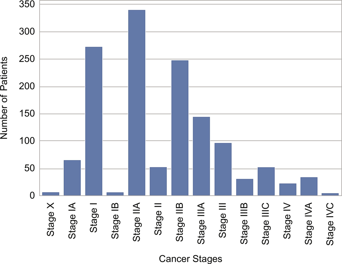
The pathological stage of the patient constitutes the target feature to be predicted. After preprocessing and cleaning, a total of 3073 samples from 1789 patients are included in our experiments. The distribution of patients per type of cancer can be seen in Fig. 3, as well as the distribution of cancer stages across all types of cancers in Fig. 4. The last figure reveals imbalance in the dataset with a majority of patients labeled as stage IIA. While gathering information from the different sources of data, not all patients have information available for all the features, therefore the datasets contain missing values for some. Missing values are also present in the target feature cancer stage, leading to unlabeled instances that will be leveraged for semisupervised classification. For those patients where more than one recorded stage of the same type of cancer is available, we kept the most advanced one.

4: Experiments and discussion
In this section, we explore the cancer stage prediction problem for breast, esophagus, and thyroid cancer through different settings. We first explore the baseline predictions obtained by the black box and white box component classifiers when working on only the labeled data. We show the influence of adding the proteomic dimension to the clinical data for the stage prediction. Second, we explore how the unlabeled data help in the semisupervised setting where all cancer types are used to build the model. Finally, we explore how unlabeled data coming from more common cancer types can help in predicting the cancer stage of more rare ones.
For the validation of our experiments, a leave one group out cross-validation was used. In this type of cross-validation, the dataset was divided in 10 disjoint groups of patients for avoiding using samples of the same patient for training and testing. Patients with missing cancer stage are not included in the test sets, they are only added to the training sets when semisupervised classification is performed. Notice that one patient can have more than one sample record and each sample constitutes an instance in the dataset (see Tables 1–4 for the number of instances).
Table 1
| blank cell | Instances | Features | RF | ||||
|---|---|---|---|---|---|---|---|
| ACC | KAPPA | SEN | SPE | AUC | |||
| BR | 1898 | Clinical | 0.44 | 0.24 | 0.45 | 0.79 | 0.69 |
| blank cell | + proteomic | 0.81 | 0.75 | 0.81 | 0.93 | 0.94 | |
| ES | 124 | Clinical | 0.25 | 0.01 | 0.25 | 0.73 | 0.51 |
| blank cell | + proteomic | 0.41 | 0.17 | 0.41 | 0.75 | 0.61 | |
| TH | 383 | Clinical | 0.60 | 0.36 | 0.60 | 0.84 | 0.77 |
| blank cell | + proteomic | 0.60 | 0.24 | 0.60 | 0.61 | 0.76 | |
| All | 2405 | Clinical | 0.43 | 0.30 | 0.43 | 0.87 | 0.74 |
| blank cell | + proteomic | 0.75 | 0.69 | 0.75 | 0.92 | 0.94 | |
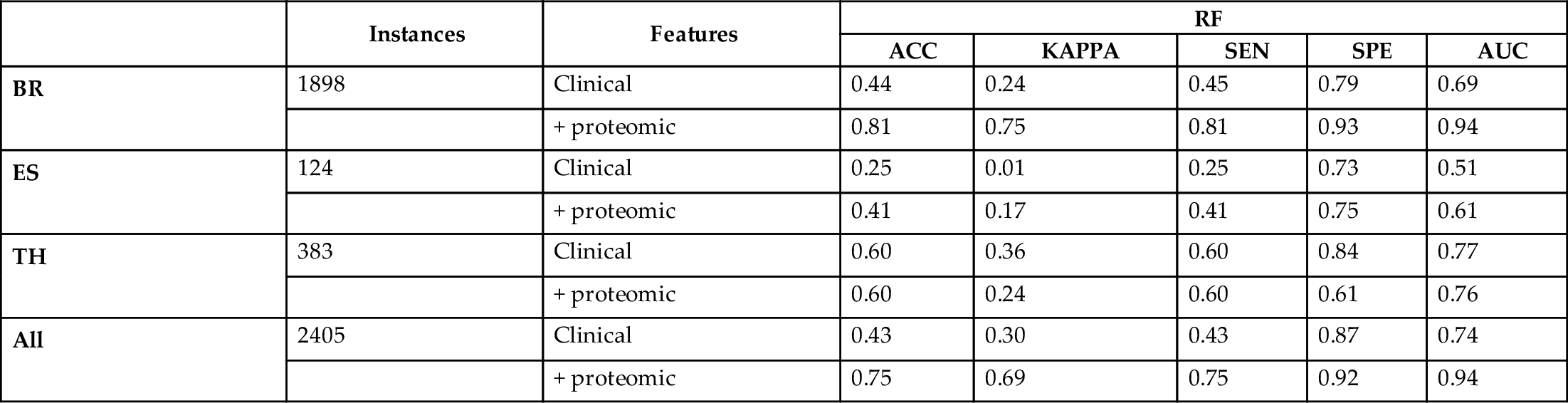
Table 2
| blank cell | Instances | Features | C4.5 | |||||
|---|---|---|---|---|---|---|---|---|
| ACC | KAPPA | SEN | SPE | AUC | Rules | |||
| BR | 1898 | Clinical | 0.46 | 0.25 | 0.46 | 0.79 | 0.70 | 94 |
| blank cell | + proteomic | 0.75 | 0.68 | 0.75 | 0.94 | 0.86 | 222 | |
| ES | 124 | Clinical | 0.30 | − 0.01 | 0.30 | 0.69 | 0.47 | 4 |
| blank cell | + proteomic | 0.23 | 0.06 | 0.23 | 0.84 | 0.46 | 28 | |
| TH | 383 | Clinical | 0.65 | 0.45 | 0.65 | 0.90 | 0.77 | 4 |
| blank cell | + proteomic | 0.59 | 0.37 | 0.59 | 0.96 | 0.64 | 40 | |
| All | 2405 | Clinical | 0.51 | 0.39 | 0.51 | 0.88 | 0.78 | 299 |
| blank cell | + proteomic | 0.67 | 0.61 | 0.67 | 0.93 | 0.82 | 325 | |
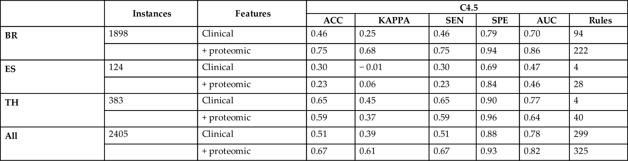
Table 3
| blank cell | Instances | Features | PART | |||||
|---|---|---|---|---|---|---|---|---|
| ACC | KAPPA | SEN | SPE | AUC | Rules | |||
| BR | 1898 | Clinical | 0.39 | 0.14 | 0.39 | 0.75 | 0.61 | 78 |
| blank cell | + proteomic | 0.77 | 0.70 | 0.77 | 0.94 | 0.86 | 149 | |
| ES | 124 | Clinical | 0.29 | − 0.04 | 0.29 | 0.68 | 0.48 | 10 |
| blank cell | + proteomic | 0.28 | 0.11 | 0.28 | 0.84 | 0.45 | 17 | |
| TH | 383 | Clinical | 0.65 | 0.46 | 0.65 | 0.90 | 0.78 | 12 |
| blank cell | + proteomic | 0.62 | 0.41 | 0.62 | 0.85 | 0.67 | 28 | |
| All | 2405 | Clinical | 0.46 | 0.34 | 0.46 | 0.87 | 0.73 | 277 |
| blank cell | + proteomic | 0.68 | 0.61 | 0.68 | 0.93 | 0.80 | 229 | |

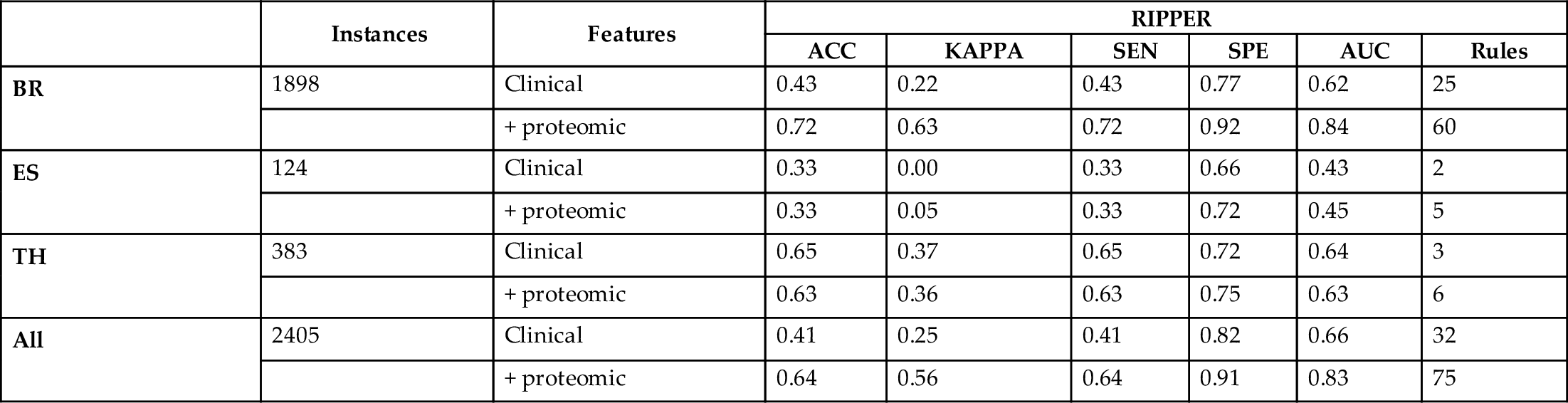
Table 4
| blank cell | Instances | Features | RIPPER | |||||
|---|---|---|---|---|---|---|---|---|
| ACC | KAPPA | SEN | SPE | AUC | Rules | |||
| BR | 1898 | Clinical | 0.43 | 0.22 | 0.43 | 0.77 | 0.62 | 25 |
| blank cell | + proteomic | 0.72 | 0.63 | 0.72 | 0.92 | 0.84 | 60 | |
| ES | 124 | Clinical | 0.33 | 0.00 | 0.33 | 0.66 | 0.43 | 2 |
| blank cell | + proteomic | 0.33 | 0.05 | 0.33 | 0.72 | 0.45 | 5 | |
| TH | 383 | Clinical | 0.65 | 0.37 | 0.65 | 0.72 | 0.64 | 3 |
| blank cell | + proteomic | 0.63 | 0.36 | 0.63 | 0.75 | 0.63 | 6 | |
| All | 2405 | Clinical | 0.41 | 0.25 | 0.41 | 0.82 | 0.66 | 32 |
| blank cell | + proteomic | 0.64 | 0.56 | 0.64 | 0.91 | 0.83 | 75 | |
The Weka library (Hall et al., 2009) was used for the implementation of random forests, decision trees, and decision lists algorithms.c Random forests consist of 100 decision trees built using a random subset of features with cardinality equal to the base-2 logarithm of the number of features. Decision trees and PART decision lists use C4.5 algorithm for generating the trees, with a parameter C = 0.25 which denotes the confidence value for performing pruning in the trees (the lower the value, the more pruning is performed). The minimum number of instances on each leaf is two. In RIPPER implementation, the training data are split into a growing set and a pruning set for performing reduced error pruning. The rule set formed from the growing set is simplified with pruning operations optimizing the error on the pruning set. The minimum allowed support of a rule is two and the data are split in three folds where one is used for pruning. Additionally, the number of optimization iterations is set to two.
Given the nature of the target attribute, the prediction problem at hand is not only an imbalance multiclass classification problem, but it is also an ordinal one. The traditional approach to deal with ordinal classification is coding the decision class into numeric values and using a regression model for the prediction. However, this limits the choice of black box and white box components to regression techniques only. Instead we use the approach described by Frank and Hall (2001), which does not require any modification of the underlying prediction algorithm. With this technique, our multiclass classification problem is transformed in several binary classifications datasets where each predictor determines the probability of the class value being greater than a given label and the greatest probability is taken as the decision. This transformation is only applied in the black box component of the SLGB without affecting the interpretability of the white box component.
4.1: Influence of clinical and proteomic data on the prediction of cancer stage
In this subsection, we explore the baseline performance of the classifiers that will be later used as components of the SLGB method. This evaluation is performed in a supervised setting, i.e., only the labeled information is considered. First, we evaluate the performance of random forests (RF), decision trees (C4.5), and decision lists algorithms PART and RIPPER on the classification of cancer stages based on the clinical data only. Later, we add the protein features for comparing how much the proteomic data brings in terms of performance. We perform this analysis for each cancer type: breast (BR), esophagus (ES), and thyroid (TH), and additionally for the entire dataset. Tables 1–4 show the results using different performance metrics. Accuracy (ACC) shows the proportion of correctly classified instances, while kappa (KAPPA) (Cohen, 1960) considers the agreement occurring by chance. This makes this measure more robust in presence of class imbalance. Other measures such as sensitivity (SEN), specificity (SPE), and area under the receiver operating characteristic curve (AUC) are also included. Since the prediction problem at hand is a multiclass classification problem, the last three measures are weighted averages of these measures for each class label. For the white box classifiers, the number of rules is measured as an indication of the size of the structure and its simplicity. The number of rules is measured for the model built based on all instances instead of individual cross-validation folds.
From the Tables 1–4, we can conclude that adding proteomic information to the clinical data substantially improves the accuracy of all classifiers in the datasets, and more evidently for breast cancer. Looking at the performance across classifiers, random forests achieve the best results in terms of accuracy. Its high kappa values indicate that despite the class imbalance, the random forest can generalize further than predicting majority classes. This is supported by high true positive and true negative rates. Overall, these results make random forests a promising base black box component for self-labeling the unlabeled data in the following experiments.
Regarding the performance of the white box base classifiers, less accuracy compared to RF is observed across datasets, which is an expected result. Nevertheless, the accuracy values obtained for the entire dataset by the three white box methods are greater than 0.64 and supported by high kappa, sensitivity, specificity, and AUC values. Regarding the number of rules, C4.5 being the most accurate comes with the largest number of rules, followed by PART. RIPPER obtains slightly less accurate results with the largest reduction in the number of rules and therefore the most transparent classifier. However, the interpretation of these three white boxes differ and can be exploited according to the needs of the user.
Comparing the results across different types of cancers, there is evidence that the limitation in data of esophagus and thyroid cancer leads to poor performance. This contrasts with the performance of the predictors trained on breast cancer data which is more abundant and better balanced across classes. In the next section, we join the data for all types of cancers and explore whether the SLGB can obtain a trade-off between performance and interpretability in the semisupervised setting.
4.2: Influence of unlabeled data on the prediction of cancer stage
In this section, we explore the performance of SLGB in the semisupervised prediction of the cancer stage. This time we incorporate 668 unlabeled instances to the learning process, in addition to the 2405 labeled ones. As stated earlier, RF will be used as base classifier for the black box component. A weighting process based on rough sets theory measures is used for amending the errors in the self-labeling process. The three white boxes presented earlier will be explored comparing their performance and interpretability. Table 5 summarizes the experiments results.
Table 5
| blank cell | ACC | KAPPA | SEN | SPE | AUC | Rules |
|---|---|---|---|---|---|---|
| SLGB (RF-C4.5) | 0.70 | 0.62 | 0.70 | 0.92 | 0.85 | 235 |
| SLGB (RF-PART) | 0.69 | 0.60 | 0.69 | 0.91 | 0.82 | 174 |
| SLGB (RF-RIPPER) | 0.63 | 0.52 | 0.63 | 0.88 | 0.83 | 26 |
| C4.5 | 0.67 | 0.61 | 0.67 | 0.93 | 0.82 | 325 |
| PART | 0.68 | 0.61 | 0.68 | 0.93 | 0.80 | 229 |
| RIPPER | 0.64 | 0.56 | 0.64 | 0.91 | 0.83 | 75 |

The performance results of white boxes from the previous section are summarized for comparison purposes.
Although the number of added unlabeled instances is not large, the SLGB still manages to improve or maintain the performance compared to their base white boxes, while reducing the number of rules needed for achieving this accuracy. The best results are observed with C4.5 as white box, where the accuracy is increased in 0.03 while the number of rules is reduced in 72%, effectively gaining in transparency.
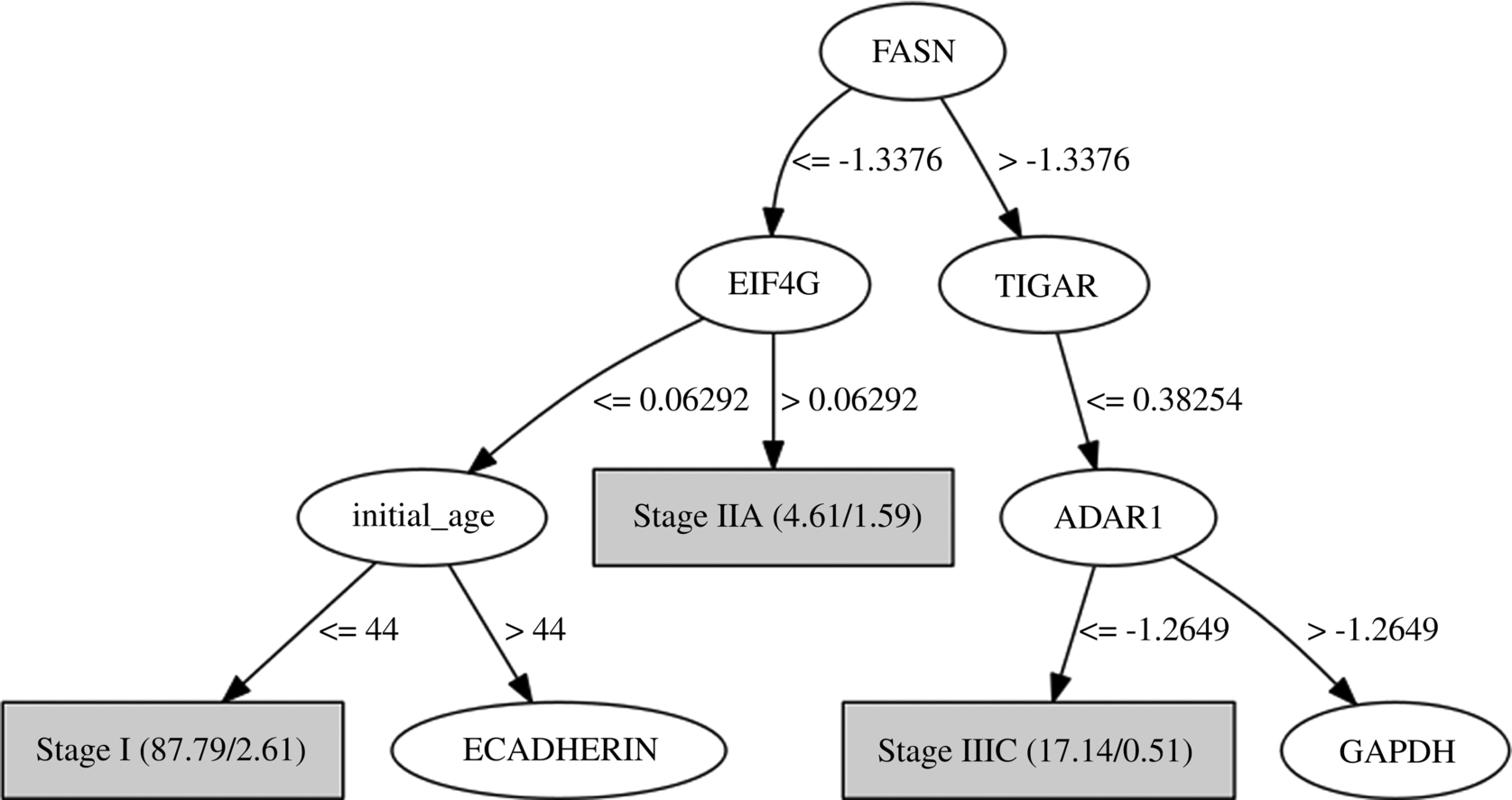
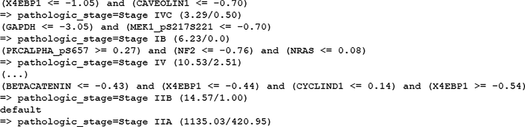
When examining the decision tree generated by the gray box model (see pruned first levels of the tree in Fig. 5), the most informative attributes detected are the proteins FASN, EIF4G, TIGAR, ADAR1, and the clinical feature “age of the initial pathologic diagnostic.” High levels of expression of FASN (fatty acid synthase) protein has been associated through several studies with the later stages of cancer, predicting poor prognosis for breast cancer among others (Buckley et al., 2017). Overexpression of EIF4G is associated with malignant transformation (Bauer et al., 2002; Fukuchi-Shimogori et al., 1997). TIGAR expression regulates the p53 tumor suppressor protein which prevents cancer development through various mechanisms (Bensaad et al., 2006; Green and Chipuk, 2006; Won et al., 2012). ADAR1 has demonstrated functional role in the RNA editing in thyroid cancer (Ramírez-Moya and Santisteban, 2020; Xu et al., 2018). PART and RIPPER rules (see Figs. 6 and 7) associate these and other features to the stages of cancer. While PART exhibits its most confident and supported rules first, RIPPER focuses in predicting the minority class. Therefore, the choice of which decision list to use must come from the need of obtaining explanations about the most common patterns or the rarest ones. These known associations support the rules learned by the machine learning models which provide potential relations that need to be further analyzed and validated clinically.

While the SLGB approach is already able to leverage the unlabeled data for improving performance and interpretability, more impressive results are commonly obtained when the number of unlabeled instances is greater than the labeled ones. In the next subsection, we study how unlabeled instances coming from more frequent types of cancers help in the classification of more rare ones.
4.3: Influence of unlabeled data on the prediction of cancer stage for rare cancer types
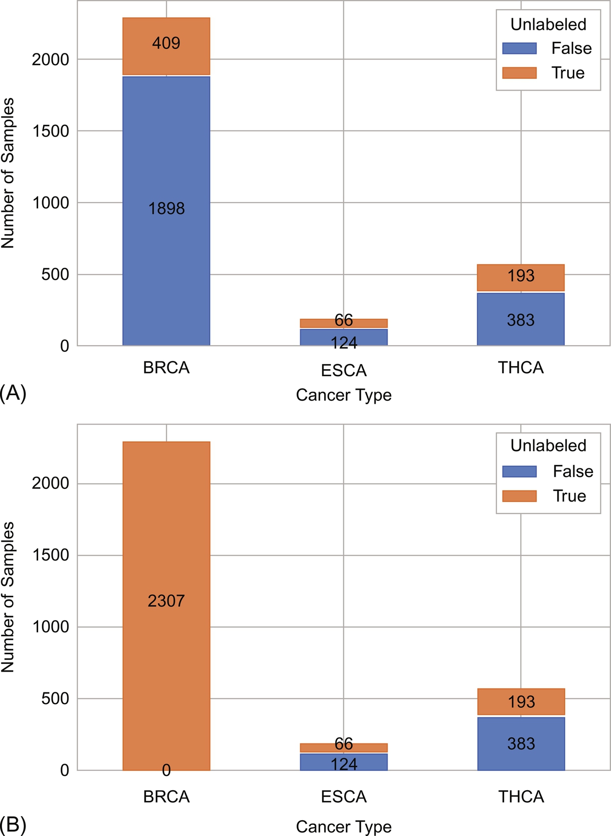
In this subsection, we study how unlabeled instances coming from a more frequent type of cancer, such as breast, help in the classification of more rare ones. For this setting, we assume that all instances from breast cancer have the cancer stage label missing. In this manner, we are studying whether unlabeled data from breast cancer helps on improving the generalization of the classifier for thyroid and esophagus cancers. Fig. 8 shows the distribution of unlabeled instances per type of cancer in the dataset as used in the previous section (Fig. 8A) and after neglecting the labels of breast cancer for the current experiment (Fig. 8B).
Next, we test how much the performance of SLGB improves on the classification of rare cancers with regard to its interpretable supervised baseline. Table 6 shows the results of the experiment using several measures of performance and the number of rules generated as an indicative of the complexity of the model. Overall, being a very imbalanced multiclass classification problem, it is challenging to obtain a high performance in terms of accuracy even for RF classifier. Nevertheless, the accuracy obtained for all classifiers is well balanced through classes as evidenced by a fair kappa value and high specificity.
Table 6
| blank cell | ACC | KAPPA | SEN | SPE | AUC | Rules |
|---|---|---|---|---|---|---|
| SLGB (RF-C4.5) | 0.57 | 0.43 | 0.57 | 0.89 | 0.73 | 80 |
| SLGB (RF-PART) | 0.57 | 0.43 | 0.57 | 0.90 | 0.73 | 47 |
| SLGB (RF-RIPPER) | 0.56 | 0.41 | 0.56 | 0.89 | 0.72 | 13 |
| RF | 0.61 | 0.48 | 0.61 | 0.90 | 0.87 | – |
| C4.5 | 0.52 | 0.37 | 0.52 | 0.90 | 0.66 | 74 |
| PART | 0.48 | 0.31 | 0.48 | 0.88 | 0.67 | 51 |
| RIPPER | 0.52 | 0.32 | 0.52 | 0.83 | 0.65 | 12 |
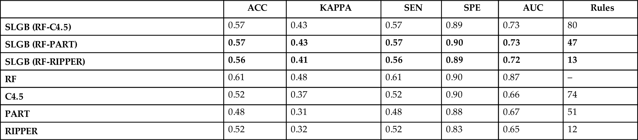
The performance results of base classifiers are shown as a baseline. The best results are highlighted in bold.
From the table we can observe that SLGB clearly outperforms its white box base classifiers for each case, with the biggest improvement using PART decision lists. At the same time, the number of rules is kept reasonably similar, without adding further complexity to the classifier and therefore keeping the transparency to some extent. The best results were obtained by SLGB using PART, and second, using RIPPER, though RIPPER needs a smaller number of rules for achieving the performance. However, the interpretation of these two classifiers differ in their focus, with PART being more appropriate for finding rules in frequent patterns and RIPPER for more rare ones as it starts from the minority class label.
5: Conclusions
In this chapter, we illustrate the application of the interpretable semisupervised classifier SLGB in the prediction of the stage of cancer patients. In a first experiment, the performance of the base classifiers conforming the self-labeling gray box indicated that joining the clinical and proteomic data from cancer patients improves the generalization ability. Later, we empirically demonstrate that the self-labeling gray box is accurate in predicting the stage of cancer by leveraging the unlabeled data already present in the dataset. We extend this experiment in simulating that all data coming from breast cancer is unlabeled, and to study how much the SLGB is able to improve its prediction on less frequent cancers such as thyroid and esophagus. In this setting, the SLGB outperformed its white box baseline classifiers while keeping the transparency (in terms of number of rules) very similar. Using random forests as a black box component and tree different alternatives as white boxes involving decision trees and rule lists allows obtaining interpretable classifiers for different scenarios. We show the form of representation of the patterns extracted by the three different white box techniques, which detect several protein expressions features which are known to play an important role in the progression of cancer. These known associations support the rules learned by the SLGB, providing potential relations that could be further analyzed clinically. In this regard, future research will explore further the validation of the patterns detected by the interpretable models by contrasting the discovered knowledge with experts’ criteria and complement it with other traditional analysis techniques. The current results pave the way for using SLGB as a tool for aiding clinicians in detecting important proteomic and clinical features that contribute to the development of advances stages in cancer.