
Chapter 22: A review of deep learning models for medical diagnosis
Seshadri Sastry Kunapulia; Praveen Chakravarthy Bhallamudib a Xinthe Technologies PVT LTD, Visakhapatnam, India
b Lumirack Solutions, Chennai, India
Abstract
Artificial intelligence (AI) is the capability of training machines to perform detection, cognitive, and diagnostic tasks on a par with humans. AI has evolved to the point that it can perform some medical diagnosis tasks similarly to human experts. We have reviewed the latest AI research in the immense field of medical science, covering various architectures and approaches, with special attention given to brain tumor analysis. This chapter discusses various deep learning architectures used to diagnose brain tumors and compares results with existing architectures. The scope of AI in medical diagnosis tasks, observations and conclusions, and future directions are also discussed. Case studies in medical diagnostics are examined, from basic clustering techniques such as K-means clustering to fuzzy, neurotrophic C-means clustering techniques and kernel graph cuts (KGCs), to advanced artificial intelligence techniques such as deep convolution neural networks (DCNs), atrous convolution neural networks (ACNs), and U-Net architectures, in order to find the area of interest in the coherent/incoherent regions. In the process, we have studied the practical advantages of using atrous convolution and its transpose in the U-Net architecture with attention mechanism instead of traditional convolution and other machine-learning approaches.
Keywords
MRI scan; Tumor; Segmentation; Deep learning; Atrous convolution
1: Motivation
Brain tumor detection/segmentation is the most challenging, as well as essential, task in many medical-image applications, because it generally involves a significant amount of data/information. There are many types of tumors (sizes and shapes). Artificial intelligence-assisted automatic/semiautomatic detection/segmentation is now playing an important role in medical diagnosis. Prior to therapies such as chemotherapy, radiotherapy, or brain surgery, the medical practitioners must validate the limits and the regions of the brain tumor as well as determine where specifically it lies and the exact affected locations. This chapter reviews various algorithms for brain tumor segmentation/detection and compares their Dice similarity coefficients (DSCs). Finally, an algorithm for brain tumor segmentation is proposed.
2: Introduction
This chapter reviews various deep learning models for tumor segmentation and proposes a technique for more efficient tumor segmentation. Magnetic resonance imaging (MRI) is a popular noninvasive technique of choice for structural brain analysis and visualization of different abnormalities in the brain. MRI provides images with high contrast and spatial resolutions for soft tissues and accessibility of multispectral images and presents no known health risks. However, identifying the pixels of organs or injuries in MRI images is among the most challenging of medical image analysis tasks, but is needed in order to deliver crucial data about the shapes and volumes of these organs or injuries.
Many researchers have examined various automated segmentation systems by applying different technologies. Researchers are employing deep learning techniques increasingly to automate these applications. Nowadays, numerous computer vision applications based on deep learning have shown improved performance, sometimes better than humans, and the applications range from recognizing objects or recognizing indicators for blood cancer and tumors in MRI scans.
Deep neural networks (DNNs) are capable of learning from unstructured data by using fine-tuning done by the backpropagation technique. The architecture of DNN has several levels to represent the features. In addition, more general information is provided at a higher level. Deep learning has progressed during the digital era, due to the availability of more massive amounts of data.
Earlier systems were built on traditional methods, such as edge detection filters and mathematical methods. Later, machine learning (ML) approaches extracting hand-crafted features became a dominant technique for an extended period. Designing and extracting appropriate features is a big concern in developing ML-assisted systems, and due to the complexities of these procedures, ML-based systems are not widely deployed. Recently, deep learning approaches came into the picture and started to demonstrate their considerable capabilities in image-processing tasks. The promising ability of deep learning approaches has placed them as the first option for image segmentation, and particularly for medical image segmentation.
Deep learning is being widely used because of its recent superior performance in many applications, such as object detection, speech recognition, facial recognition, and medical imaging.(Bar et al., 2015). Many researchers have pursued works on applications of deep learning in ultrasound (Shen et al., 2017), medical imaging (Baumgartner et al., 2017; Bergamo et al., 2011; Cai et al., 2017; Chen et al., 2017, 2015, 2016a), magnetic resonance imaging (Chen et al., 2016b, c), medical image segmentation, such as (Litjens et al., 2017) and (Shen et al., 2017), and electroencephalograms (Cheng et al., 2016). Recurrent neural network (RNN) is an alternative DL technique that is perfect for evaluating sequential data (for example, text and speech) because it has an inner state of memory that can be used for storage of data about prior data points. LSTM (Hochreiter and Schmidhuber, 1997) is a variation of RNN with better memory retention, as compared to conventional RNN. It is used for recognition of speech, captioning of images, and machine translations. Generative adversarial networks (GANs) and their various forms are another rising DL architecture containing generator and discriminator networks that are trained by backpropagation. The generator network artificially generates more realistic data cases that attempt to imitate the training data, whereas the discriminator network attempts to determine whether the artificially generated samples belong to training samples. GANs have shown great possibilities in medical image applications, like the reconstruction of medical imaging, e.g., compressed sensing MRI reconstruction (Mardani et al., 2017). Shen et al. (Shen et al., 2017) reviewed applications of deep learning on different kinds of medical image analysis problems. In the process, Zhou (2019) has reviewed deep learning architectures for different multimodality datasets as they can provide multiinformation of a specific tissue or a cell or an organ.
Before automated analysis can be carried out, preprocessing steps are needed to make the images appear more similar. Typical preprocessing steps for structural brain MRI include: (1) registration, (2) registration, (3) bias field correction, (4) intensity normalization, (5) noise reduction.
Registration is the alignment of the images to a common coordinate system/space (Shen et al., 2017). Interpatient registration is a process to align the images of different sequences, to obtain a multichannel representation for each location within the brain. Interpatient image registration aids in standardizing the MR images onto a standard stereotaxic space, commonly the Montreal Neurological Institute (MNI) space. Klein et al. (2009) ranked 14 algorithms applied to brain image registration according to three completely independent analyses (permutation tests, one-way ANOVA tests, and indifference-zone ranking). They derived three almost identical top rankings of the methods. The algorithms ART, SyN, IRTK, and SPM's DARTEL Toolbox gave the best results based on overlap and distance measures.
Skull stripping is an important step in MRI brain imaging applications, referring to the removal of the noncerebral tissues. The main problem in skull-stripping is the segmentation of the noncerebral and intracranial tissues due to their homogeneous intensities. Many researchers have proposed algorithms for skull-stripping. Smith (2002) proposed and developed an automated method for segmenting magnetic resonance head images into the brain and nonbrain, called Brain Extraction Tool (BET). Iglesias et al. (2011) developed a robust, learning-based brain extraction system (ROBEX). Statistical Parametric Mapping (SPM), with a number of improved versions, is open source software commonly used in MRI analysis (Iglesias et al., 2011; Ashburner and Friston, 2005). The process of mapping intensities of all images into a standard reference scale is known as intensity normalization, with intensities generally scaled between 0 and 4095. Nyúl and Udupa (1999) proposed a two-step postprocessing method for standardizing the intensity scale in such a way that for the same MR protocol and body region,
Noise reduction is the reduction of the locally variant Rician noise observed in MR images (Coupe et al., 2008). With the advent of deep learning techniques, some of the preprocessing steps became less critical for the final segmentation performance. Gondara (2016) proposed convolutional denoising autoencoders to denoise images.
Akkus et al. (2017) surveyed various segmentation algorithms used for MRI scans and presented them. Razzak et al. (2018) presented an overview of various deep learning methods proposed under medical image processing in the literature. Vovk et al. (2007) has reviewed a paper on different image enhancement techniques based on correction of intensity inhomogeneity for MRI images with different qualitative and quantitative approaches. Menze et al. (2014) proposed the multimodal brain tumor image segmentation benchmark (BRATS) for brain tumor segmentation, which in turn used by many researchers for Image Segmentation from basic Convolution Methods to advanced U-Nets. One such a paper is proposed by Pereira et al. (2016). Işın et al. (2016) presented a review of MRI-based brain tumor image segmentation using deep learning methods. Hall et al. (1992) compared neural network and fuzzy clustering techniques in segmenting magnetic resonance images of the brain. Krizhevsky et al. (2012) proposed deep learning architecture for image classification. Litjens et al. (2017) presented a survey on deep learning in medical image analysis. Xian et al. (2018) proposed algorithms on automatic breast ultrasound image segmentation. Kitahara et al. (2019) proposed a deep learning approach for dynamic chest radiography. Chang et al. (2019) proposed a deep learning method for the detection of complete anterior cruciate ligament tear. Ronneberger et al. (2015) proposed U-Net, convolutional networks for biomedical image segmentation. Long et al. (2015) proposed fully convolutional networks for semantic segmentation. Dong et al. (2017) proposed automatic brain tumor detection and segmentation using U-Net based fully convolutional networks. Çiçek et al. (2016) proposed the 3D U-Net: learning dense volumetric segmentation from the sparse annotation. Ioffe and Szegedy (2015) proposed accelerating deep network training by reducing the internal covariate shift. Wang et al. (2018) proposed automatic brain tumor segmentation using cascaded anisotropic convolutional neural networks.
A review of all these deep learning algorithms for medical image segmentation has been done previously (Ronneberger et al., 2015) with explanations as to how they can be useful in segmenting even the minor regions of the incoherent or fuzzy structures of the tumors in the medical image, along with their challenges in implementation for limited annotated datasets. But the main challenge in designing a deep neural network architecture is the vanishing gradient problem during the training of deep networks. So, to overcome this problem, a feed-forward connection from one layer to all the subsequent layers has been done using Densenets, which not only adds regularization effects but also reduces the problem of overfitting on small datasets. Inspired by the Densenets, Dolz (2019) proposed a multimodal technique called HyperDense-Net to improve the accuracy of brain lesion segmentation with the help of multimodal settings in the network. In dealing with the overfitting or vanishing gradients problem, An (2019) proposed an adaptive dropout technique in his spliced convolution neural network for image depth calculation and segmentation and he measured his model accuracy using the Dice score and Jaccard index for the spine web dataset. As no rigid segmentation is required for PET images, Cheng and Liu (2017) has proposed a combination of Convolution Neural Networks (to extract internal features) and Recurrent Neural Networks (to classify these features) is used for Alzheimer's disease diagnosis.
However, the traditional strided convolution techniques (such as in deep convolution networks (DCNs) or fully connected neural networks (FCNNs) (An, 2020)) are being replaced for image segmentation by atrous (i.e., dilated) kernels or convolution, with holes (which introduces a dilation rate to the convolution layers that defines the spacing between the kernel values). This technique can be used in DCNs (Zhou, 2020) in order to achieve a maximum accuracy in segmenting medical images, with a trade-off of greater memory and segmentation time. However, the usage of this atrous convolution layer in a simple encoder network has been proposed by Gu (2019), in which the network consists of a simple decoder with pretrained Resnet32 and a dense atrous convolution (DAC) block with use of a residual multikernel pooling (RMP) layer instead of a dense U-Net architecture to improve the segmentation accuracy. In recent research, different models with U-Net architecture, such as single U-Net architecture with atrous spatial pyramidal pooling (ASPP) (Pengcheng, 2020) and double U-Net architecture (Jha, 2020) with a connection of VGG-19 squeeze and excite block with ASPP network architectures, have been proposed and that outperformed medical image segmentation, with better accuracy and low false positive rate. Dice ratio or Jaccard index can be used to find the accuracy of the segmented image, or it can be done with the help of modern machine learning parameters such as precision and recall.
The results of the preceding papers mostly confirmed that the use of atrous, a.k.a. dilated, convolution techniques, or convolution with holes, in medical image segmentation along with the U-Net architecture brings up the most probabilistic detection on medical image segmentation or tumor segmentation, even though they are in a coherent or incoherent structure, when compared to the other techniques. So, in this review, we strongly suggest that the structure of multiscale atrous convolution in the U-Net architecture gives better and more accurate results in detecting minute tumors in real time, with the trade-off of time and memory.
3: MRI Segmentation
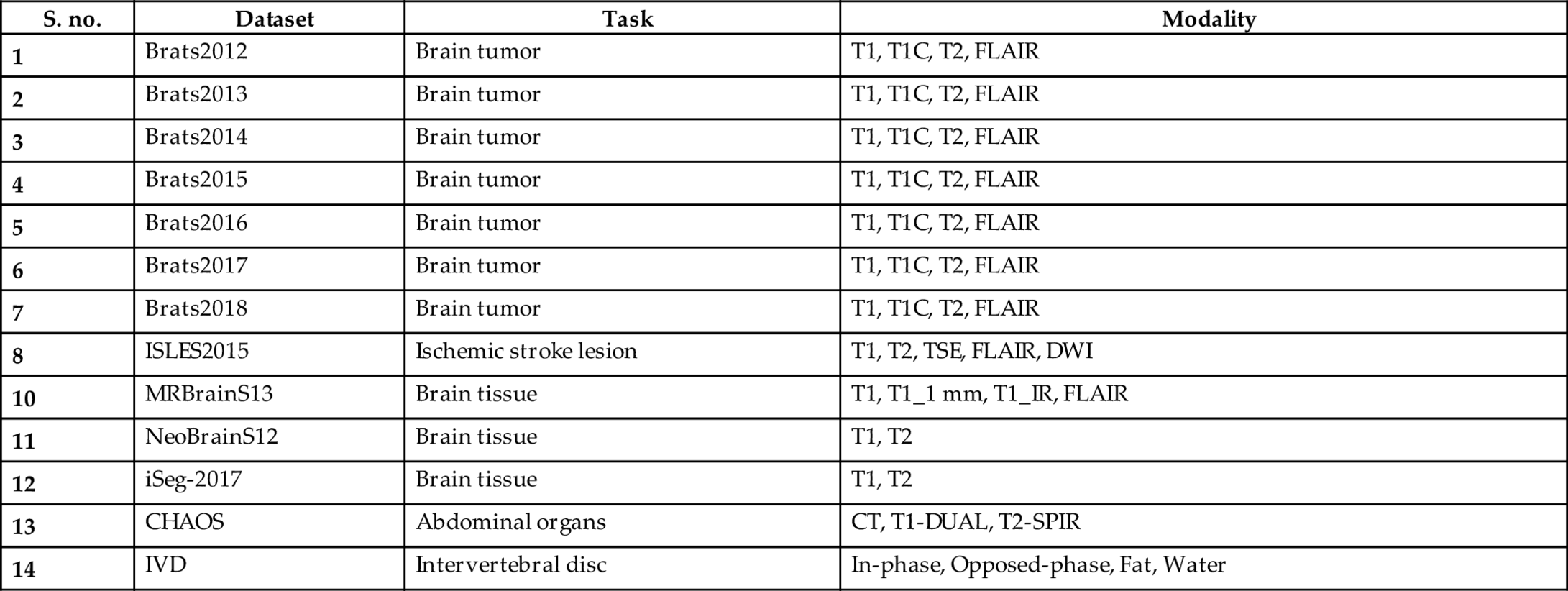
Image segmentation is an essential step for brain tumor analysis of MRI images. In the present scenario, the human expert performs tumor segmentation manually. This manual segmentation is a very time-consuming, tedious task, usually involving lengthier procedures, and the results are very dependent on human expertise. Moreover, these results vary from expert to expert and generally are not reproducible by the same expert. Thus automatic segmentation and reproducible segmentation methods are very much in demand. MRI segmentation is used to provide a more accurate classification for the subtypes of brain tumors and inform the subsequent diagnosis. It allows precise delineation that is crucial in radiotherapy or surgical planning. In this chapter, we review various architectures used to segment brain tissues and compare their Dice sensitivity coefficient (DSC). Table 1 shows the list of datasets available: T1 (spin-lattice relaxation), T1_1mm (3D T1-weighted scan), T1_IR (multislice T1-weighted inversion recovery scan registered to the T2 FLAIR), T1C (T1-contrasted), T2 (spin-spin relaxation), proton density (PD) contrast imaging, diffusion MRI (dMRI), and fluid attenuation inversion recovery (FLAIR) pulse sequences. The BraTS dataset provides four modalities for each patient: T1, T2, T1c, and FLAIR diffusion-weighted imaging (DWI) are designed to detect the random movements of water protons. DWI is a suitable method for detecting acute stroke. Computed tomography (CT), T1-DUAL (in-phase) (40 datasets), and T2-SPIR (opposed phase) The contrast between these modalities gives an almost unique signature to each tissue type. MRBrainS13 and ISLES2015 provide four and five modalities, respectively.
Table 1
| S. no. | Dataset | Task | Modality |
|---|---|---|---|
| 1 | Brats2012 | Brain tumor | T1, T1C, T2, FLAIR |
| 2 | Brats2013 | Brain tumor | T1, T1C, T2, FLAIR |
| 3 | Brats2014 | Brain tumor | T1, T1C, T2, FLAIR |
| 4 | Brats2015 | Brain tumor | T1, T1C, T2, FLAIR |
| 5 | Brats2016 | Brain tumor | T1, T1C, T2, FLAIR |
| 6 | Brats2017 | Brain tumor | T1, T1C, T2, FLAIR |
| 7 | Brats2018 | Brain tumor | T1, T1C, T2, FLAIR |
| 8 | ISLES2015 | Ischemic stroke lesion | T1, T2, TSE, FLAIR, DWI |
| 10 | MRBrainS13 | Brain tissue | T1, T1_1 mm, T1_IR, FLAIR |
| 11 | NeoBrainS12 | Brain tissue | T1, T2 |
| 12 | iSeg-2017 | Brain tissue | T1, T2 |
| 13 | CHAOS | Abdominal organs | CT, T1-DUAL, T2-SPIR |
| 14 | IVD | Intervertebral disc | In-phase, Opposed-phase, Fat, Water |
4: Deep learning architectures used in diagnostic brain tumor analysis
4.1: Convolutional neural networks or convnets
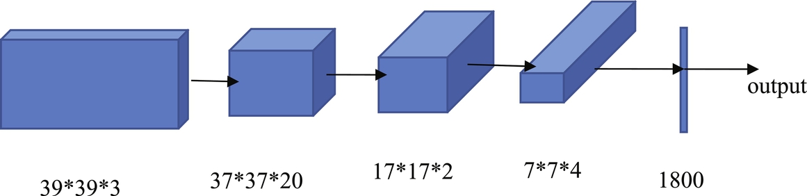
Convolutional neural networks are also deep feedforward networks that are widely used in classification, recognition, and detection tasks, such as object detection, object recognition (Jiang et al., 2013; Wang et al., 2019), handwriting recognition (Havaei, 2017), and image classification (Dong, 2017; Pinto et al., 2015; Havaei et al., 2016; Kamnitsas et al., 2017). The difference between the fully connected feedforward neural networks (FCNs) and the deep convolution neural networks (DCNNs) is that the adjacent layers are connected in different ways. The DCNN only has some nodes connected between the adjacent two layers, while the FCN has all nodes connected between the adjacent two layers. The biggest problem with using an FCN is that there are too many parameters/features for the network. Increasing the features will only lead to increased complexity, reduced speed, and overfitting problems. To reduce overfitting, it is required to reduce the parameters given to the network. Therefore convolutional neural networks were proposed to achieve this goal. Convolutional neural networks consist of convolutional and pooling layers. In the convolutional layer, only a small patch of the previous layer is used as the input of each node in the convolutional layer, and the size of the small patch is often 3*3 or 5*5. The convolutional layer attempts to analyze each small patch of the neural network in depth, which results in the higher abstraction of feature representation—the pooling layer followed by the convolutional layer. The pooling layer reduces the size of the output of the convolutional layer; thus this combination of convolutional layers and the pooling layer can reduce the number of parameters in the network. So, pooling layers not only speed up the calculation but also prevent overfitting. In general, there are two types of convolution neural network architectures, according to the different connection modes of the different convolutional layers. One is to connect 2D convolutional layers in series, such as VGG-16, VGG-19 (Zhou, 2020), ResNET (Gu, 2019), and INCEPTION-NETt (Pengcheng, 2020). Fig. 1 shows an example architecture of the convolutional neural network and the other is 3D Multi-Scale CNN for MRI brain lesion segmentation which is proposed by Kamnitsas et al. (2016) and Kleesiek et al. (2016).
4.2: Stacked autoencoders
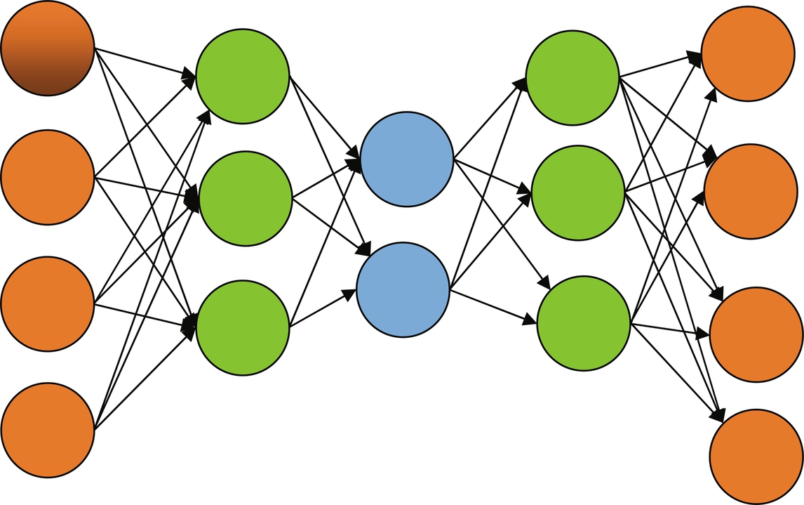
An autoencoder is a type of artificial neural network used to learn efficient data coding in an unsupervised manner. There are two parts in an autoencoder: the encoder and the decoder. The encoder is used to generate a reduced feature representation from an initial input x by a hidden layer h. The decoder is used to reconstruct the initial input from the encoder's output by minimizing the loss function. The autoencoder converts high-dimensional data to low-dimensional data. Therefore the autoencoder is especially useful in noise removal, feature extraction, compression, and similar tasks. There are three types of autoencoder: the sparse autoencoder (Zhou, 2020), the denoising autoencoder (Gu, 2019; Majumdar, 2019; Vaidhya, 2015) and the contractive autoencoder (Pengcheng, 2020). Sparse autoencoders are typically used to learn features for another task such as classification. Denoising autoencoders create a noisy copy of the input data by adding some noise to the input. This prevents the autoencoders from copying the input to the output without learning features of the data. The objective of a contractive autoencoder is to have a robust learned representation that is less sensitive to small variations in the data. Robustness of the data description is created by applying a penalty term to the loss function. A contractive autoencoder is another regularization technique, just like sparse and denoising autoencoders. However, this regularizing corresponds to the Frobenius norm of the Jacobian matrix of the encoder activations concerning the input. The Frobenius norm of the Jacobian matrix for the hidden layer is calculated concerning input, and it is the sum of the squares of all elements. Fig. 2 shows an autoencoder example.
4.3: Deep belief networks
The Boltzmann machine (Ioffe and Szegedy, 2015; Wang et al., 2018; Ronneberger et al., 2015) is derived from statistical physics and is a modeling method based on energy functions that describe the high-order interaction between variables. Although the Boltzmann machine is relatively complex, it has a relatively complete physical interpretation and a strict mathematical statistics theory. The Boltzmann machine is an asymmetric coupled random feedback binary unit neural network, which includes a visible layer and multiple hidden layers. The nodes of the Boltzmann computer can be divided into visible units and hidden units. In a Boltzmann machine, the visible and invisible units represent the random neural network learning model. The weights between two units in the model are used to describe the correlation between the corresponding two units. A restricted Boltzmann machine (Dolz, 2019; An, 2019) is a unique form, which only includes a visible layer and a hidden layer. Unlike feedforward neural networks, the connections between the nodes of the hidden layer and the visible layer's nodes in the restricted Boltzmann machines can be bidirectionally connected. Compared to Boltzmann machines, since the restricted Boltzmann machines only have one hidden layer, they have faster calculation speed and better flexibility. In general, restricted Boltzmann machines have two main functions: (1) Similar to autoencoders, restricted Boltzmann machines are used to reduce the dimension of data; (2) Restricted Boltzmann machines are used to obtain a weight matrix, which is used as the initial input of other neural networks. Similar to stacked autoencoders, deep belief networks (An, 2020; Zhou, 2020; Gu, 2019; Pengcheng, 2020) are also neural networks with multiple restricted Boltzmann machine layers.
Furthermore, in deep belief networks, the next layer's input comes from the previous layer's output. Deep belief networks adopt the hierarchical unsupervised greedy pretraining method (An, 2020) to pretrain each restricted Boltzmann machine hierarchically. The obtained results in this study were used as the initial input of the supervised learning probability model, whose learning performance improved significantly. In addition to the segmentation tasks, a classification model of various brain tumors on MRI images have been done with the help of Deep Belief Networks have been done by Ahmed (2019).
4.4: 2D U-Net
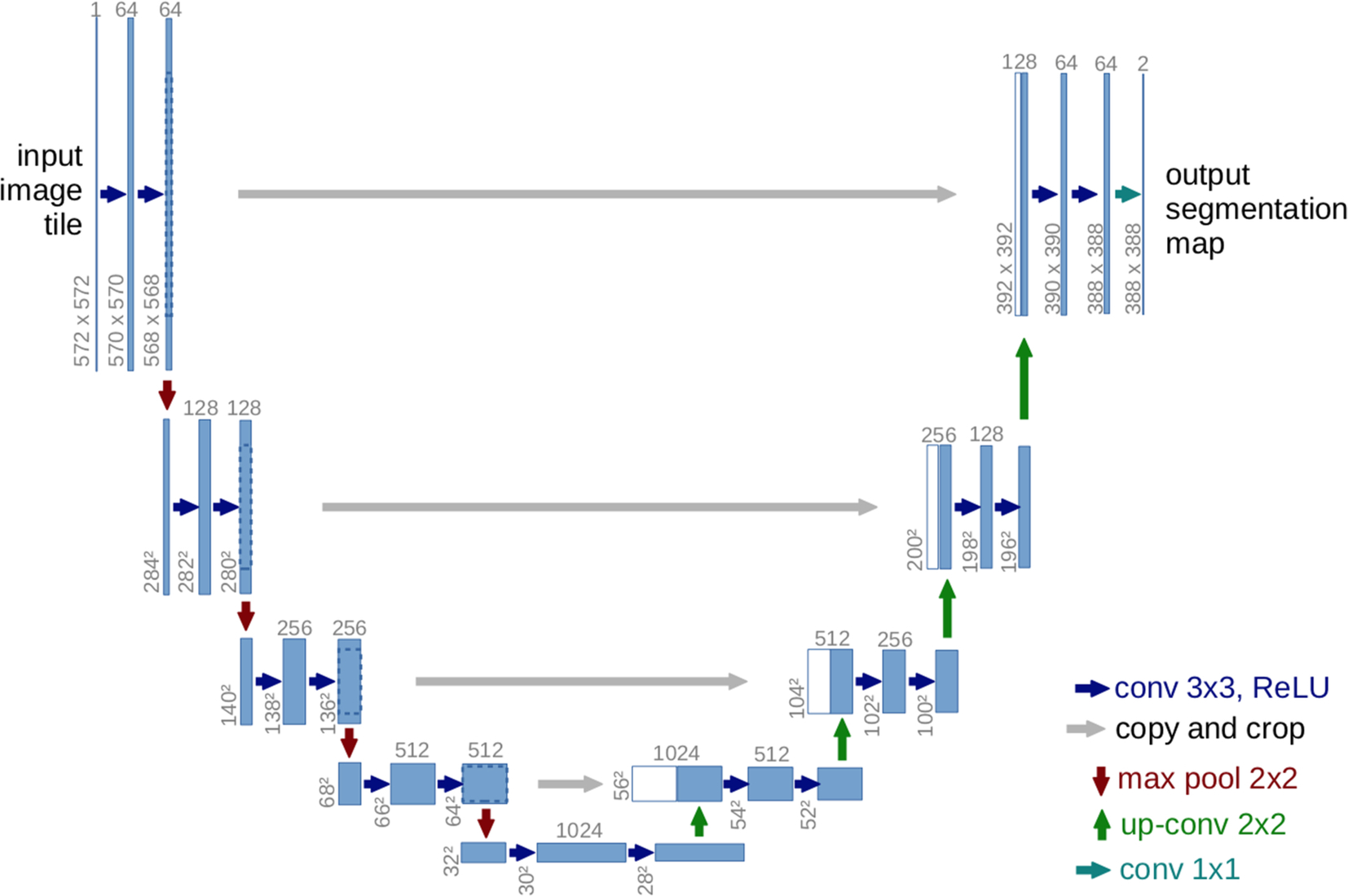
The U-Net was proposed by Olaf Ranneberger et al. for biomedical image segmentation (Ronneberger et al., 2015). It is an improvement on the fully convolutional neural networks for semantic segmentation (Hesamian et al., 2019; Dong, 2017). U-Net follows the idea of an autoencoder to find a latent representation of a lower dimension than the input used for the segmentation task architecture, containing two parts. The first part is the encoder part or contraction path, used to capture the image's context. An encoder consists of convolutional and pooling layers. The second path, known as a decoder, is an expanding path, which is used to enable localization using transposed convolutions. U-Net contains only fully convolutional layers and does not contain any dense layer, because it can accept images of any size (Hesamian et al., 2019). Fig. 3 shows an example of the U-Net architecture.
4.5: 3D U-Net
The 3D U-Net architecture is similar to the U-Net (He, 2016). It comprises an analysis path to the left and a synthesis path to the right. The whole image is analyzed in a contracting way, and subsequent expansions produce the final segmentation. In the analysis path of U-Net, each layer contains two 3 × 3 × 3 convolution layers, each followed by a ReLU layer, and then a 2 × 2 × 2 max pooling layer with strides of two in each dimension. In the synthesis path of U-Net, each layer consists of a 2 × 2 × 2 up-convolution by strides of value two in each dimension, followed by two 3 × 3 × 3 convolution layers, each followed by a ReLU activation function. Shortcut connections from the analysis path to the synthesis path provide the high-resolution features. In the last segment, a convolution of size 1 × 1 × 1 reduces the number of output channels to three labels. 3D U-Net has all the operations in 3D and uses batch normalization, which was shown to improve the training convergence. An example of this separable 3D U-Net Architecture on MRI images for brain tumor segmentation has been proposed by Chen et al. (2018) which has shown a good result in tumor segmentation when comparing to the 2D architectures.
4.6: Cascaded anisotropic network
The cascaded anisotropic network (Wang et al., 2017) consists of three convolutional neural networks (CNNs) that segment each of three subregions sequentially: 1. tumor, 2. tumor core, and 3. enhancing tumor. Hence, anisotropic convolutions perform well on 3D MRI, but result in higher complexity and memory consumption. The fusion of the CNN outputs in three orthogonal views is used to enhance the brain tumor segmentation. The cascaded anisotropic network uses three CNNs to hierarchically and sequentially segment whole tumor, tumor core, and enhancing tumor core. These CNNs are referred to as WNet, TNet, and ENet, respectively, and they follow the hierarchical structure of the tumor subregions. WNet and TNet have the same architecture, while ENet only uses one down-sampling layer due to the smaller input size. The WNet takes the full MRI. As input and segments, the first region: whole tumor. A corresponding bounding box is computed and used as the input of the TNet that segments the tumor core similarly used for the ENet. The bounding boxes allow a restriction of the segmentation region and minimize false positives and false negatives. One of the cascade’s drawbacks is that it is not an end-to-end method and thus training and testing time are more extended than with the other methods. Fig. 4 shows the architecture of the cascaded anisotropic network.
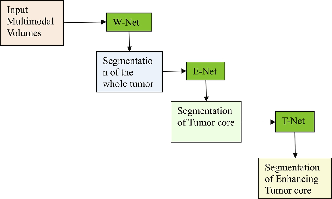
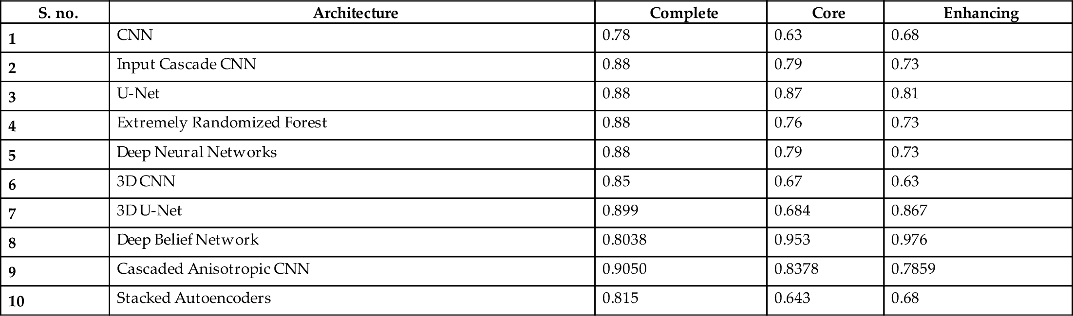
Table 2 shows a comparison of the Dice sensitivity coefficient (DSC) of the complete tumor, the core of the tumor, and the enhanced core of tumors. TP- True Positives, FP- False Positives, FN- False Negatives. The formula for DSC is given by ![]() .
.
Table 2
| S. no. | Architecture | Complete | Core | Enhancing |
|---|---|---|---|---|
| 1 | CNN | 0.78 | 0.63 | 0.68 |
| 2 | Input Cascade CNN | 0.88 | 0.79 | 0.73 |
| 3 | U-Net | 0.88 | 0.87 | 0.81 |
| 4 | Extremely Randomized Forest | 0.88 | 0.76 | 0.73 |
| 5 | Deep Neural Networks | 0.88 | 0.79 | 0.73 |
| 6 | 3D CNN | 0.85 | 0.67 | 0.63 |
| 7 | 3D U-Net | 0.899 | 0.684 | 0.867 |
| 8 | Deep Belief Network | 0.8038 | 0.953 | 0.976 |
| 9 | Cascaded Anisotropic CNN | 0.9050 | 0.8378 | 0.7859 |
| 10 | Stacked Autoencoders | 0.815 | 0.643 | 0.68 |
5: Deep learning tools applied to MRI images
In recent years, based on the previously described general deep learning methods, some deep learning tools applied to MRI have also been developed. They are briefly introduced as follows.
- BrainNet: This tool was developed based on TensorFlow and aims to train deep neural networks to segment grey matter and white matter from brain MRIs.
- LiviaNET: LiviaNET (Dolz et al., 2018) was developed using Theano, aiming to train 3D fully convolutional neural networks to segment subcortical brain on MRI.
- DIGITS: This tool was also developed to rapidly train accurate deep neural networks for image segmentation, classification, and tissue detection tasks. For example, DIGITS is used to perform Alzheimer's disease prediction by using MRI and obtains good results (Sarraf and Tofigh, 2016).
- resnet CNN MRI adni: This tool was developed to train residual and convolutional neural networks (CNNs) to perform automatic detection and classification of MRIs.
- mrbrain: This tool was developed to train convolutional neural networks by using MRIs to predict the age of humans.
- DeepMedic: DeepMedic was developed using Theano and aims to train multiscale 3D CNNs for brain lesion segmentation from MRI.
6: Proposed framework
Based on a comparison of DSCs of various architectures in Table 2, cascaded anisotropic CNN performed well on the BraTs dataset compared to other architectures. Further, U-Net also performed reasonably well on all three types of data: complete, core, and enhanced. We are confident that enhancing the architecture of U-Net would improve its performance. We propose a U-Net architecture with atrous, a.k.a. dilated, convolution layers (convolution with holes) for medical image segmentation. The proposed technique exhibits the most accurate probabilistic detection on medical image segmentation/tumor segmentation even though they are incoherent structures, when compared to the other techniques. Hence, we propose a multiscale atrous convolution U-Net architecture with batch normalization and he-norm as a kernel initializer (as the dataset contains fewer images and different tumor sizes in each image). The architecture of our proposed model is shown in Fig. 5.
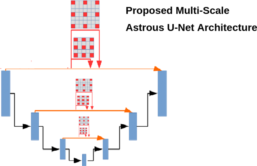
In this architecture, we used an exponential increase of receptive fields with an increased kernel parameter linearly, without losing the characteristics of the image, i.e., resolution or coverage. Let f1, f2, f3, …, fn be the discrete functions such that they belong to any real dimension (R) of data and k1, k2, …, kn are the kernels such that in a multiscale atrous convolution the size of each element in the receptive field increases exponentially with a linear increase of n elements by the factor of (2n + 2 − 1)×(2n + 2 − 1), such that if n = 0 the size of the kernel becomes 3*3 and if n = 1 the size becomes 7*7, and so on. This exponential increase of the kernel does not affect the resolution or coverage of the image and it works well if we have a less image segmentation dataset.
In general, the activation functions, such as either relu or tanh, may sometimes lead to either vanishing gradients or saturation problems. We generally preferred he-normalization as a kernel initializer, as it introduces zero mean and common variance between the predecessors when compared to other initializers, such as “Xavier normal/uniform” and “uniform/random” initializers. To optimize our network, we used a batch normalization between every multiscaling dilated convolution layer to converge faster, even though with high learning rates this causes the gradients to move towards the direction of the prediction faster. In the proposed U-Net architecture, instead of up-sampling, we used atrous convolution transpose. Up-sampling has no trainable parameters and it only repeats the rows and columns in the data. In the convolution transpose layer, both convolution and up-sampling are used. In our proposed technique, we used multiscale atrous convolution transpose, which would utilize different filter sizes in transpose convolution and finds the depth of the image with greater detail. The proposed algorithm, as expected, performed well on the BraTS dataset compared to U-Net and cascaded anisotropic CNN. The Dice sensitivity coefficient (DSC) of the proposed architecture complete tumor was 0.91, the core of the tumor was 0.89, and the enhanced core of tumors was 0.82.
7: Conclusion and outlook
In summary, this chapter has aimed to provide valuable insights for researchers about applying deep learning architectures in the field of MRI research. Deep learning architectures are widely applied to MRI processing and analysis in registration, bias field correction, intensity normalization, noise reduction, image detection, image segmentation, and image classification. Although deep learning approaches perform well on MRI, there are still many limitations and challenges that need to be met and overcome. In designing deep learning approaches, significant limitations are dataset size and class imbalance. Generally, deep learning approaches require larger datasets for better results—namely, the size of the MRI. The dataset is limited due to its cost in image acquisition processes and privacy considerations; further, many disease-related MRIs are rarely found. Therefore the size of the datasets with MRIs are often small. So, it is overly complicated to train deep neural networks and get the desired performance with the class imbalance in the images.
However, there are many strategies for dealing with imbalanced datasets, such as resampling techniques, which include random undersampling and random oversampling. Random undersampling removes examples randomly in the majority class, aiming to balance class distribution by indiscriminantly eliminating majority class examples. This elimination of examples is done until the majority and minority class examples are balanced out.
Oversampling increases the number of examples in the minority class by randomly copying and replicating them to increase samples of the minority class in the dataset. In cluster-based oversampling, the K-means unsupervised algorithm is applied to the minority and majority classes separately. This process is done to identify groups/clusters in the dataset. Subsequently, each group is oversampled, such that all groups of the same class have the same number of examples, and all classes have the same size. Due to replicating sample model overfits, to avoid overfitting in informed oversampling, new synthetic similar instances of the minority class are created and added to the dataset.
Transfer learning is an approach used in deep learning to learn new tasks based on knowledge earned on older tasks. Transfer learning is widely applied to deal with limited dataset size and class imbalance. Transfer learning consists of selecting a pretrained network, followed by a fine-tuning process, i.e., choosing a suitable pretrained deep learning architecture and tuning its corresponding hyperparameters for a particular application. It is difficult to select an architecture straightaway and tune its hyperparameters for a particular application. This remains an unsolved problem. Presently, most researchers are pursuing experimental experience to address the previously mentioned problems—the size of the MRI. The dataset may no longer be a problem due to the continuous advancements of medical data. Moreover, new progress and understanding of deep learning concepts may result in choosing a suitable deep learning architecture and its corresponding hyperparameters for a particular application more appropriately. Shortly, we may expect more remarkable achievements through deep learning on MRI analysis.
8: Future directions
Despite the many improvements in artificial intelligence/machine learning, there are still many inadequacies. Mostly these issues are identified with the current methods, which are not adjusted to the larger, more varied, and increasingly complex datasets, which may affect the accuracy of tumor segmentation. Further research should investigate and propose new architectures, layers, or even activations to develop a next-generation segmentation for tumor detection.