2.4.1 Primitive Events

Before experimenting, we assumed that the probability of rolling a one is one out of six. That number comes from #ways this event can occur#of different events. We can test our understanding of that ratio by asking, “What is the probability of rolling an odd number?” Well, using Roman numerals to indicate the outcomes of a roll, the odd numbers in our space of events are I, III, V. There are three of these and there are six total primitive events. So, we have P(odd)=36=12. Fortunately, that gels with our intuition.

We can approach this calculation a different way: an odd can occur in three ways and those three ways don’t overlap. So, we can add up the individual event probabilities: P(odd)=P(I)+P(III)+P(V)=16+16+16=36=12. We can get probabilities of compound events by either counting primitive events or adding up the probabilities of primitive events. It’s the same thing done in two different ways.

This basic scenario gives us an in to talk about a number of important aspects of probability:

• The sum of the probabilities of all possible primitive events in a universe is 1.

  P(I) + P(II) + P(III) + P(IV) + P(V) + P(VI) = 1.

• The probability of an event not occurring is 1 minus the probability of it occurring. P(even) = 1 – P(not even) = 1 – P(odd). When discussing probabilities, we often write “not” as ¬, as in P(¬even). So, P(¬even) = 1 – P(even).

• There are nonprimitive events. Such a compound event is a combination of primitive events. The event we called odd joined together three primitive events.

• A roll will be even or odd, but not both, and all rolls are either even or odd. These two compound events cover all the possible primitive events without any overlap. So, P(even) + P(odd) = 1.

Compound events are also recursive. We can create a compound event from other compound events. Suppose I ask, “What is the probability of getting an odd or a value greater than 3 or both?” That group of events, taken together, is a larger group of primitive events. If I attack this by counting those primitive events, I see that the odds are odd = {I, III, V} and the big values are big = {IV, V, VI}. Putting them together, I get {I, III, IV, V, VI} or 56. The probability of this compound event is a bit different from the probability of odds being 12 and the probability of greater-than-3 being 12. I can’t just add those probabilities. Why not? Because I’d get a sum of one—meaning we covered everything—but that only demonstrates the error. The reason is that the two compound events overlap: they share primitive events. Rolling a five, V, occurs in both subgroups. Since they overlap, we can’t just add the two together. We have to add up everything in both groups individually and then remove one of whatever was double- counted. The double-counted events were in both groups—they were odd and big. In this case, there is just one double-counted event, V. So, removing them looks like P(odd) + P(big) – P(odd and big). That’s 12+12−16=56.

2.4.2 Independence

If we roll two dice, a few interesting things happen. The two dice don’t communicate or act on one another in any way. Rolling a I on one die does not make it more or less likely to roll any value on the other die. This concept is called independence: the two events—rolls of the individual dice—are independent of each other.

For example, consider a different set of outcomes where each event is the sum of the rolls of two dice. Our sums are going to be values between 2 (we roll two Is) and 12 (we roll two VIs). What is the probability of getting a sum of 2? We can go back to the counting method: there are 36 total possibilities (6 for each die, times 2) and the only way we can roll a total of 2 is by rolling two Is which can only happen one way. So, P(2)=136 We can also reach that conclusion—because the dice don’t communicate or influence each other—by rolling I on die 1 and I on die 2, giving P(I1)P(I2)=16⋅16=136. If events are independent, we can multiply their probabilities to get the joint probability of both occurring. Also, if we multiply the probabilities and we get the same probability as the overall resulting probability we calculated by counting, we know the events must be independent. Independent probabilities work both ways: they are an if-and-only-if.

We can combine the ideas of (1) summing the probabilities of different events and (2) the independence of events, to calculate the probability of getting a total of three P(3). Using the event counting method, we figure that this event can happen in two different ways: we roll (I, II) or we roll (II, I) giving 2/36 = 1/18. Using probability calculations, we can write:

Phew, that was a lot of work to verify the answer. Often, we can make use of shortcuts to reduce the number of calculations we have to perform. Sometimes these shortcuts are from knowledge of the problem and sometimes they are clever applications of the rules of probability we’ve seen so far. If we see multiplication, we can mentally think about the two-dice scenario. If we have a scenario like the dice, we can multiply.

2.4.3 Conditional Probability

Let’s create one more scenario. In classic probability-story fashion, we will talk about two urns. Why urns? I guess that, before we had buckets, people had urns. So, if you don’t like urns, you can think about buckets. I digress.

The first urn U_I has three red balls and one blue ball in it. The second urn U_II has two red balls and two blue balls. We flip a coin and then we pull a ball out of an urn. If the coin comes up heads, we pick from U_I; otherwise, we pick from U_II. We end up at U_I half the time and then we pick a red ball 34 of those times. We end up at U_II the other half of the time and we pick a red ball 24 of those times. This scenario is like wandering down a path with a few intersections. As we walk along, we are presented with a different set of options at the next crossroads.

If we sketch out the paths, it looks like Figure 2.1. If we count up the possibilities, we will see that under the whole game, we have five red outcomes and three blue outcomes. P(red)=58. Simple, right? Not so fast, speedy! This counting argument only works when we have equally likely choices at each step. Imagine we have a very wacky coin that causes me to end up at Urn I 999 out of 1000 times: then our chances of picking a red ball would end up quite close to the chance of just picking a red ball from Urn I. It would be similar to almost ignoring the existence of Urn II. We should account for this difference and, at the same time, make use of updated information that might come along the way.

If we play a partial game and we know that we’re at Urn I—for example, after we’ve flipped a head in the first step—our odds of picking a red ball are different. Namely, the probability of picking a red ball—given that we are picking from Urn I—is 34. In mathematics, we write this as P(red|UI)=34. The vertical bar, |, is read as “given”. Conditioning—a commonly verbed noun in machine learning and statistics—constrains us to a subset of the primitive events that could possibly occur. In this case, we condition on the occurrence of a head on our coin flip.

How often do we end up picking a red ball from Urn I? Well, to do that we have to (1) get to Urn I by flipping a head, and then (2) pick a red ball. Since the coin doesn’t affect the events in Urn I—it picked Urn I, not the balls within Urn I—the two are independent and we can multiply them to find the joint probability of the two events occurring. So, P(red and UI)=P(red|UI)P(UI)=12⋅34=38. The order here may seem a bit weird. I’ve written it with the later event—the event that depends on U_I—first and the event that kicks things off, U_I, second. This order is what you’ll usually see in written mathematics. Why? Largely because it places the | U_I next to the P(U_I). You can think about it as reading from the bottom of the diagram back towards the top.

Since there are two nonoverlapping ways to pick a red ball (either from Urn I or from Urn II), we can add up the different possibilities. Just as we did for Urn I, for Urn II we have P(red and UII)=P(red|UII)P(UII)=12⋅24=28. Adding up the alternative ways of getting red balls, either out of Urn I or out of Urn II, gives us: P(red)=P(red|UI)P(UI)+P(red|UII)P(UII)=38+28=58. Mon dieu! At least we got the same answer as we got by the simple counting method. But now, you know what that important vertical bar, P(|), means.

2.4.4 Distributions

There are many different ways of assigning probabilities to events. Some of them are based on direct, real-world experiences like dice and cards. Others are based on hypothetical scenarios. We call the mapping between events and probabilities a probability distribution. If you give me an event, then I can look it up in the probability distribution and tell you the probability that it occurred. Based on the rules of probability we just discussed, we can also calculate the probabilities of more complicated events. When a group of events shares a common probability value—like the different faces on a fair die—we call it a uniform distribution. Like Storm Troopers in uniform, they all look the same.

There is one other, very common distribution that we’ll talk about. It’s so fundamental that there are multiple ways to approach it. We’re going to go back to coin flipping. If I flip a coin many, many times and count the number of heads, here’s what happens as we increase the number of flips:

In [5]:

Click here to view code image

import scipy.stats as ss

b = ss.distributions.binom
for flips in [5, 10, 20, 40, 80]:
    # binomial with .5 is result of many coin flips
    success = np.arange(flips)
    our_distribution = b.pmf(success, flips, .5)
    plt.hist(success, flips, weights=our_distribution)
plt.xlim(0, 55);

If I ignore that the whole numbers are counts and replace the graph with a smoother curve that takes values everywhere, instead of the stair steps that climb or descend at whole numbers, I get something like this:

In [6]:

Click here to view code image

b = ss.distributions.binom
n = ss.distributions.norm

for flips in [5, 10, 20, 40, 80]:
    # binomial coin flips
    success = np.arange(flips)
    our_distribution = b.pmf(success, flips, .5)
    plt.hist(success, flips, weights=our_distribution)

    # normal approximation to that binomial
    # we have to set the mean and standard deviation
    mu      = flips * .5,
    std_dev = np.sqrt(flips * .5 * (1-.5))

    # we have to set up both the x and y points for the normal
    # we get the ys from the distribution (a function)
    # we have to feed it xs, we set those up here
    norm_x = np.linspace(mu-3*std_dev, mu+3*std_dev, 100)
    norm_y = n.pdf(norm_x, mu, std_dev)
    plt.plot(norm_x, norm_y, 'k');

plt.xlim(0, 55);

You can think about increasing the number of coin flips as increasing the accuracy of a measurement—we get more decimals of accuracy. We see the difference between 4 and 5 out of 10 and then the difference between 16, 17, 18, 19, and 20 out of 40. Instead of a big step, it becomes a smaller, more gradual step. The step-like sequences become progressively better approximated by the smooth curves. Often, these smooth curves are called bell-shaped curves—and, to keep the statisticians happy, yes, there are other bell-shaped curves out there. The specific bell-shaped curve that we are stepping towards is called the normal distribution.

The normal distribution has three important characteristics:

1. Its midpoint has the most likely value—the hump in the middle.

2. It is symmetric—can be mirrored—about its midpoint.

3. As we get further from the midpoint, the values fall off more and more quickly.

There are a variety of ways to make these characteristics mathematically precise. It turns out that with suitable mathese and small-print details, those characteristics also lead to the normal distribution—the smooth curve we were working towards! My mathematical colleagues may cringe, but the primary feature we need from the normal distribution is its shape.

2.5.1 Weighted Average

You might be familiar with a simple average—and now you’re wondering, “What is a weighted average?” To help you out, the simple average—also called the mean—is an equally weighted average computed from a set of values. For example, if I have three values (10, 20, 30), I divide up my weights equally among the three values and, presto, I get thirds: 1310+1320+1330. You might be looking at me with a distinct side eye, but if I rearrange that as 10+20+303 you might be happier. I simply do sum(values)/3: add them all up and divide by the number of values. Look what happens, however, if I go back to the more expanded method:

In [14]:

Click here to view code image

values  = np.array([10.0, 20.0, 30.0])
weights = np.full_like(values, 1/3) # repeated (1/3)

print("weights:", weights)
print("via mean:", np.mean(values))
print("via weights and dot:", np.dot(weights, values))

weights: [0.3333 0.3333 0.3333]
via mean: 20.0
via weights and dot: 20.0

We can write the mean as a weighted sum—a sum product between values and weights. If we start playing around with the weights, we end up with the concept of weighted averages. With weighted averages, instead of using equal portions, we break the portions up any way we choose. In some scenarios, we insist that the portions add up to one. Let’s say we weighted our three values by 12,14,14. Why might we do this? These weights could express the idea that the first option is valued twice as much as the other two and that the other two are valued equally. It might also mean that the first one is twice as likely in a random scenario. These two interpretations are close to what we would get if we applied those weights to underlying costs or quantities. You can view them as two sides of the same double-sided coin.

In [15]:

Click here to view code image

values  = np.array([10,  20,  30])
weights = np.array([.5, .25, .25])

np.dot(weights, values)

Out[15]:

17.5

One special weighted average occurs when the values are the different outcomes of a random scenario and the weights represent the probabilities of those outcomes. In this case, the weighted average is called the expected value of that set of outcomes. Here’s a simple game. Suppose I roll a standard six-sided die and I get $1.00 if the die turns out odd and I lose $.50 if the die comes up even. Let’s compute a dot product between the payoffs and the probabilities of each payoff. My expected outcome is to make:

In [16]:

Click here to view code image

                  # odd, even
payoffs = np.array([1.0, -.5])
probs   = np.array([ .5,  .5])
np.dot(payoffs, probs)

Out[16]:

0.25

Mathematically, we write the expected value of the game as E(game) = Σ_i p_iv_i with p being the probabilities of the events and v being the values or payoffs of those events. Now, in any single run of that game, I’ll either make $1.00 or lose $.50. But, if I were to play the game, say 100 times, I’d expect to come out ahead by about $25.00—the expected gain per game times the number of games. In reality, this outcome is a random event. Sometimes, I’ll do better. Sometimes, I’ll do worse. But $25.00 is my best guess before heading into a game with 100 tosses. With many, many tosses, we’re highly likely to get very close to that expected value.

Here’s a simulation of 10000 rounds of the game. You can compare the outcome with np.dot(payoffs, probs) * 10000.

In [17]:

Click here to view code image

def is_even(n):
    # if remainder 0, value is even
    return n % 2 == 0

winnings = 0.0
for toss_ct in range(10000):
    die_toss = np.random.randint(1, 7)
    winnings += 1.0 if is_even(die_toss) else -0.5
print(winnings)

2542.0

2.5.2 Sums of Squares

One other, very special, sum-of-products is when both the quantity and the value are two copies of the same thing. For example, 5 · 5 + (–3). (–3) + 2 · 2 + 1 · 1 = 5² + 3² + 2² + 1² = 25 + 9 + 4 + 1 = 39. This is called a sum of squares since each element, multiplied by itself, gives the square of the original value. Here is how we can do that in code:

In [18]:

Click here to view code image

values = np.array([5, -3, 2, 1])
squares = values * values # element-wise multiplication
print(squares,
      np.sum(squares),  # sum of squares. ha!
      np.dot(values, values), sep="
")

[25 9 4 1]
39
39

If I wrote this mathematically, it would look like: dot(values,values)=∑iυiυi=∑iυi2.

2.5.3 Sum of Squared Errors

There is another very common summation pattern, the sum of squared errors, that fits in here nicely. In this case of mathematical terminology, the red herring is both red and a herring. If I have a known value actual and I have your guess as to its value predicted, I can compute your error with error = predicted – actual.

Now, that error is going to be positive or negative based on whether you over- or underestimated the actual value. There are a few mathematical tricks we can pull to make the errors positive. They are useful because when we measure errors, we don’t want two wrongs—overestimating by 5 and underestimating by 5—to cancel out and make a right! The trick we will use here is to square the error: an error of 5 → 25 and an error of –5 → 25. If you ask about your total squared error after you’ve guessed 5 and –5, it will be 25 + 25 = 50.

In [19]:

Click here to view code image

errors = np.array([5, -5, 3.2, -1.1])
display(pd.DataFrame({'errors':errors,
                      'squared':errors*errors}))

So, a squared error is calculated by error² = (predicted - actual)². And we can add these up with Σi(predictedi−actuali)2=Σierrori2. This sum reads left to right as, “the sum of (open paren) errors which are squared (close paren).” It can be said more succinctly: the sum of squared errors. That looks a lot like the dot we used above:

In [20]:

np.dot(errors, errors)

Out[20]:

61.45

Weighted averages and sums of squared errors are probably the most common summation forms in machine learning. By knowing these two forms, you are now prepared to understand what’s going on mathematically in many different learning scenarios. In fact, much of the notation that obfuscates machine learning from beginners—while that same notation facilitates communication amongst experts!—is really just compressing these summation ideas into fewer and fewer symbols. You now know how to pull those ideas apart.

You might have a small spidey sense tingling at the back of your head. It might be because of something like this: c² = a² + b². I can rename or rearrange those symbols and get distance2=len12+len22ordistance=run2+rise2=Σixi2. Yes, our old friends—or nemeses, if you prefer—Euclid and Pythagoras can be wrapped up as a sum of squares. Usually, the a and b are distances, and we can compute distances by subtracting two values—just like we do when we compare our actual and predicted values. Hold on to your seats. An error is just a length—a distance—between an actual and a predicted value!

2.6.1 Lines

Let’s talk about the cost of going to a concert. I hope that’s suitably nonacademic. To start with, if you drive a car to the concert, you have to park it. For up to 10 (good) friends going to the show, they can all fit in a minivan—packed in like a clown car, if need be. The group is going to pay one flat fee for parking. That’s good, because the cost of parking is usually pretty high: we’ll say $40. Let’s put that into code and pictures:

In [21]:

Click here to view code image

people = np.arange(1, 11)
total_cost = np.ones_like(people) * 40.0

ax = plt.gca()

ax.plot(people, total_cost)
ax.set_xlabel("# People")
ax.set_ylabel("Cost
(Parking Only)");

In a math class, we would write this as total_cost = 40.0. That is, regardless of the number of people—moving back and forth along the x-axis at the bottom—we pay the same amount. When mathematicians start getting abstract, they reduce the expression to simply y = 40. They will talk about this as being “of the form” y = c. That is, the height or the y-value is equal to some constant. In this case, it’s the value 40 everywhere. Now, it doesn’t do us much good to park at the show and not buy tickets—although there is something to be said for tailgating. So, what happens if we have to pay $80 per ticket?

In [22]:

Click here to view code image

people = np.arange(1, 11)
total_cost = 80.0 * people + 40.0

Graphing this is a bit more complicated, so let’s make a table of the values first:

In [23]:

Click here to view code image

# .T (transpose) to save vertical space in printout
display(pd.DataFrame({'total_cost':total_cost.astype(np.int)},
                     index=people).T)

And we can plot that, point-by-point:

In [24]:

Click here to view code image

ax = plt.gca()
ax.plot(people, total_cost, 'bo')
ax.set_ylabel("Total Cost")
ax.set_xlabel("People");

So, if we were to write this in a math class, it would look like:

total_cost = ticket_cost × people + parking_cost

Let’s compare these two forms—a constant and a line—and the various ways they might be written in Table 2.1.

I want to show off one more plot that emphasizes the two defining components of the lines: m and b. The m value—which was the $80 ticket price above—tells how much more we pay for each person we add to our trip. In math-speak, it is the rise, or increase in y for a single-unit increase in x. A unit increase means that the number of people on the x-axis goes from x to x + 1. Here, I’ll control m and b and graph it.

In [25]:

Click here to view code image

# paint by number
# create 100 x values from -3 to 3
xs = np.linspace(-3, 3, 100)

# slope (m) and intercept (b)
m, b = 1.5, -3

ax = plt.gca()

ys = m*xs + b
ax.plot(xs, ys)

ax.set_ylim(-4, 4)
high_school_style(ax) # helper from mlwpy.py

ax.plot(0, -3,'ro') # y-intercept
ax.plot(2,  0,'ro') # two steps right gives three steps up

# y = mx + b with m=0 gives y = b
ys = 0*xs + b
ax.plot(xs, ys, 'y');

Since our slope is 1.5, taking two steps to the right results in us gaining three steps up. Also, if we have a line and we set the slope of the line m to 0, all of a sudden we are back to a constant. Constants are a specific, restricted type of horizontal line. Our yellow line which passes through y = −3 is one.

We can combine our ideas about np.dot with our ideas about lines and write some slightly different code to draw this graph. Instead of using the pair (m, b), we can write an array of values w = (w₁, w₀). One trick here: I put the w₀ second, to line up with the b. Usually, that’s how it is written in mathese: the w₀ is the constant.

With the ws, we can use np.dot if we augment our xs with an extra column of ones. I’ll write that augmented version of xs as xs_p1 which you can read as “exs plus a column of ones.” The column of ones serves the role of the 1 in y = mx + b. Wait, you don’t see a 1 there? Let me rewrite it: y = mx + b = mx + b · 1. See how I rewrote b → b · 1? That’s the same thing we need to do to make np.dot happy. dot wants to multiply something times w₁ and something times w₀. We make sure that whatever gets multiplied by w₀ is a 1.

I call this process of tacking on a column of ones the plus-one trick or +1 trick and I’ll have more to say about it shortly. Here’s what the plus-one trick does to our raw data:

In [26]:

Click here to view code image

# np.c_[] lets us create an array column-by-column
xs    = np.linspace(-3, 3, 100)
xs_p1 = np.c_[xs, np.ones_like(xs)]

# view the first few rows
display(pd.DataFrame(xs_p1).head())

Now, we can combine our data and our weights very concisely:

In [27]:

Click here to view code image

w  = np.array([1.5, -3])
ys = np.dot(xs_p1, w)

ax = plt.gca()
ax.plot(xs, ys)

# styling
ax.set_ylim(-4, 4)
high_school_style(ax)
ax.plot(0, -3,'ro') # y-intercept
ax.plot(2, 0,'ro'); # two steps to the right should be three whole steps up

Here are the two forms we used in the code: ys = m*xs + b and ys = np.dot(xs_p1, w). Mathematically, these look like y = mx + b and y = wx⁺. Here, I’m using x⁺ as an abbreviation for the x that has ones tacked on to it. The two forms defining ys mean the same thing. They just have some differences when we implement them. The first form has each of the components standing on its own. The second form requires x⁺ to be augmented with a 1 and allows us to conveniently use the dot product.

2.6.2 Beyond Lines

We can extend the idea of lines in at least two ways. We can progress to wiggly curves and polynomials—equations like f(x) = x³ + x² + x + 1. Here, we have a more complex computation on one input value x. Or, we can go down the road to multiple dimensions: planes, hyperplanes, and beyond! For example, in f(x, y, z) = x + y + z we have multiple input values that we combine together. Since we will be very interested in multivariate data—that’s multiple inputs—I’m going to jump right into that.

Let’s revisit the rock concert scenario. What happens if we have more than one kind of item we want to purchase? For example, you might be surprised to learn that people like to consume beverages at concerts. Often, they like to consume what my mother affectionately refers to as “root beer.” So, what if we have a cost for parking, a cost for the tickets, and a cost for each root beer our group orders. To account for this, we need a new formula. With rb standing for root beer, we have:

total_cost = ticket_cost × number_people + rb_cost × number_rbs + parking_cost

If we plug in some known values for parking cost, cost per ticket, and cost per root beer, then we have something more concrete:

total_cost = 80 × number_people + 10 × number_rbs + 40

With one item, we have a simple two-dimensional plot of a line where one axis direction comes from the input “how many people” and the other comes from the output “total cost”. With two items, we now have two how many’s but still only one total_cost, for a total of three dimensions. Fortunately, we can still draw that somewhat reasonably. First, we create some data:

In [28]:

Click here to view code image

number_people = np.arange(1, 11) # 1-10 people
number_rbs    = np.arange(0, 20) # 0-19 rootbeers

# numpy tool to get cross-product of values (each against each)
# in two paired arrays. try it out: np.meshgrid([0, 1], [10, 20])
# "perfect" for functions of multiple variables
number_people, number_rbs = np.meshgrid(number_people, number_rbs)

total_cost = 80 * number_people + 10 * number_rbs + 40

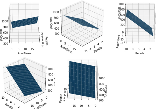
We can look at that data from a few different angles—literally. Below, we show the same graph from five different viewpoints. Notice that they are all flat surfaces, but the apparent tilt or slope of the surface looks different from different perspectives. The flat surface is called a plane.

In [29]:

Click here to view code image

# import needed for 'projection':'3d'
from mpl_toolkits.mplot3d import Axes3D
fig,axes = plt.subplots(2, 3,
                        subplot_kw={'projection':'3d'},
                        figsize=(9, 6))

angles = [0, 45, 90, 135, 180]
for ax,angle in zip(axes.flat, angles):
    ax.plot_surface(number_people, number_rbs, total_cost)
    ax.set_xlabel("People")
    ax.set_ylabel("RootBeers")
    ax.set_zlabel("TotalCost")
    ax.azim = angle

# we don't use the last axis
axes.flat[-1].axis('off')
fig.tight_layout()

It is pretty straightforward, in code and in mathematics, to move beyond three dimensions. However, if we try to plot it out, it gets very messy. Fortunately, we can use a good old-fashioned tool—that’s a GOFT to those in the know—and make a table of the outcomes. Here’s an example that also includes some food for our concert goers. We’ll chow on some hotdogs at $5 per hotdog:

total_cost = 80 × number_people + 10 × number_rbs + 5 × number_hotdogs + 40

We’ll use a few simple values for the counts of things in our concert-going system:

In [30]:

Click here to view code image

number_people  = np.array([2, 3])
number_rbs     = np.array([0, 1, 2])
number_hotdogs = np.array([2, 4])

costs = np.array([80, 10, 5])

columns = ["People", "RootBeer", "HotDogs", "TotalCost"]

I pull off combining several numpy arrays in all possible combinations, similar to what itertools’s combinations function does, with a helper np_cartesian_product. It involves a bit of black magic, so I’ve hidden it in mlwpy.py. Feel free to investigate, if you dare.

In [31]:

Click here to view code image

counts = np_cartesian_product(number_people,
                              number_rbs,
                              number_hotdogs)

totals = (costs[0] * counts[:, 0] +
          costs[1] * counts[:, 1] +
          costs[2] * counts[:, 2] + 40)

display(pd.DataFrame(np.c_[counts, totals],
                     columns=columns).head(8))

The assignment to totals—on lines 6–8 in the previous cell—is pretty ugly. Can we improve it? Think! Think! There must be a better way! What is going on there? We are adding several things up. And the things we are adding come from being multiplied together element-wise. Can it be? Is it a dot product? Yes, it is.

In [32]:

Click here to view code image

costs  = np.array([80, 10, 5])
counts  = np_cartesian_product(number_people,
                              number_rbs,
                              number_hotdogs)

totals = np.dot(counts, costs) + 40
display(pd.DataFrame(np.column_stack([counts, totals]),
                     columns=columns).head(8))

Using the dot product gets us two wins: (1) the line of code that assigns to total is drastically improved and (2) we can more or less arbitrarily extend our costs and counts without modifying our calculating code at all. You might notice that I tacked the +40 on there by hand. That’s because I didn’t want to go back to the +1 trick—but I could have.

Incidentally, here’s what would have happened in a math class. As we saw with the code-line compression from repeated additions to dot, details often get abstracted away or moved behind the scenes when we break out advanced notation. Here’s a detailed breakdown of what happened. First, we abstract by removing detailed variable names and then replacing our known values by generic identifiers:

We take this one step further in code by replacing the wx sums with a dot product:

The weird [3, 2, 1] subscript on the w indicates that we aren’t using all of the weights. Namely, we are not using the w₀ in the left-hand term. w₀ is in the right-hand term multiplying 1. It is only being used once. The final coup de grâce is to perform the +1 trick:

To summarize, instead of y = w₃x₃ + w₂x₂ + w₁x₁ + w₀, we can write y = wx⁺.

2.9.1 Back to 1D versus 2D

However, when we use a mix of 1D and 2D inputs, things are more confusing because the input arrays are not taken at face value. There are two important consequences for us: (1) the order matters in multiplying a 1D and a 2D array and (2) we have to investigate the rules np.dot follows for handling the 1D array.

In [40]:

Click here to view code image

col_vec = np.arange(0, 50, 10).reshape(5, 1)
row_vec = np.arange(0, 5).reshape(1, 5)

oned_vec = np.arange(5)

np.dot(oned_vec, col_vec)

Out[40]:

array([300])

If we trade the order, Python blows up on us:

In [41]:

Click here to view code image

try:
    np.dot(col_vec, oned_vec) # *boom*
except ValueError as e:
    print("I went boom:", e)

Click here to view code image

I went boom: shapes (5,1) and (5,) not aligned: 1 (dim 1) != 5 (dim 0)

So, np.dot(oned_vec, col_vec) works and np.dot(col_vec, oned_vec) fails. What’s going on? If we look at the shapes of the guilty parties, we can get a sense of where things break down.

In [42]:

Click here to view code image

print(oned_vec.shape,
      col_vec.shape, sep="
")

(5,)
(5, 1)

You might consider the following exercise: create a 1D numpy array and look at its shape using .shape. Transpose it with .T. Look at the resulting shape. Take a minute to ponder the mysteries of the NumPy universe. Now repeat with a 2D array. These might not be entirely what you were expecting.

np.dot is particular about how these shapes align. Let’s look at the row cases:

In [43]:

Click here to view code image

print(np.dot(row_vec, oned_vec))
try: print(np.dot(oned_vec, row_vec))
except: print("boom")

[30]
boom

Here is a summary of what we found:

For the working cases, we can see what happens if we force-reshape the 1D array:

In [44]:

Click here to view code image

print(np.allclose(np.dot(oned_vec.reshape(1, 5), col_vec),
                  np.dot(oned_vec,               col_vec)),
      np.allclose(np.dot(row_vec, oned_vec.reshape(5, 1)),
                  np.dot(row_vec, oned_vec)))

True True

Effectively, for the cases that work, the 1D array is bumped up to (1, 5) if it is on the left and to (5, 1) if it is on the right. Basically, the 1D receives a placeholder dimension on the side it shows up in the np.dot. Note that this bumping is not using NumPy’s full, generic broadcasting mechanism between the two inputs; it is more of a special case.

Broadcasting two arrays against each other in NumPy will result in the same shape whether you are broadcasting a against b or b against a. Even so, you can mimic np.dot(col_vec, row_vec) with broadcasting and multiplication. If you do that, you get the “big array” result: it’s called an outer product.

With all of that said, why do we care? Here’s why:

In [45]:

D = np.array([[1, 3],
              [2, 5],
              [2, 7],
              [3, 2]])
weights = np.array([1.5, 2.5])

This works:

In [46]:

np.dot(D,w)

Out[46]:

array([ -7.5, -12. , -18. , -1.5])

This fails:

In [47]:

try:
    np.dot(w,D)
except ValueError:
    print("BOOM. :sadface:")

BOOM. :sadface:

And sometimes, we just want the code to look like our math:

What do we do if we don’t like the interface we are given? If we are willing to (1) maintain, (2) support, (3) document, and (4) test an alternative, then we can make an interface that we prefer. Usually people only think about the implementation step. That’s a costly mistake.

Here is a version of dot that plays nicely with a 1D input as the first argument that is shaped like a column:

In [48]:

Click here to view code image

def rdot(arr,brr):
    'reversed-argument version of np.dot'
    return np.dot(brr,arr)
rdot(w, D)

Out[48]:

array([ -7.5, -12. , -18. , -1.5])

You might complain that we are going through contortions to make the code look like the math. That’s fair. Even in math textbooks, people will do all sorts of weird gymnastics to make this work: w might be transposed. In NumPy, this is fine, if it is 2D. Unfortunately, if it is only a 1D NumPy array, transposing does nothing. Try it yourself! Another gymnastics routine math folks will perform is to transpose the data—that is, they make each feature a row. Yes, really. I’m sorry to be the one to tell you about that. We’ll just use rdot—short for “reversed arguments to np.dot”—when we want our code to match the math.

Dot products are ubiquitous in the mathematics of learning systems. Since we are focused on investigating learning systems through Python programs, it is really important that we (1) understand what is going on with np.dot and (2) have a convenient and consistent form for using it. We’ll see rdot in our material on linear and logistic regression. It will also play a role in several other techniques. Finally, it is fundamental in showing the similarities of a wide variety of learning algorithms.

2.11.1 Summary

We covered a lot of ideas in this chapter and laid the groundwork to talk about learning in an intelligent way. In many cases, we won’t be diving into mathematical details of learning algorithms. However, when we talk about them, we will often appeal to probability, geometry, and dot products in our descriptions. Hopefully, you now have better intuitions about what these terms and symbols mean—particularly if no one has taken the time to explain them to you in a concrete fashion before.

2.11.2 Notes

While we took an intuitive approach to describing distributions, they have concrete mathematical forms which can be extended to multiple dimensions. The discrete uniform distribution looks like:

Here, k is the number of possible events—six for a typical die or two for a coin flip. The equation for the normal distribution is

The e, combined with a negative power, is responsible for the fast dropoff away from the center. v_m, a magic value, is really just there to make sure that all the possibilities sum up to one like all good distributions: it is υm=2π but I won’t quiz you on that. The center and spread are normally called the mean and standard deviation and written with μ and σ which are the lowercase Greek mu and sigma. The normal distribution shows up everywhere in statistics: in error functions, in binomial approximations (which we used to generate our normal shapes), and in central limit theorems.

Python uses 0-based indexing while mathematicians often use 1-based indexing. That’s because mathematicians are generally counting things and computer scientists have historically cared about offsets: from the start, how many steps do I need to move forward to get to the item I need? If I’m at the start of a list or an array, I have to take zero steps to get the first item: I’m already there. A very famous computer scientist, Edsger Dijkstra, wrote an article called “Why numbering should start at zero.” Check it out if you are interested and want to win on a computer-science trivia night.

In my mathematical notation, I’m following classic Python’s lead and letting both ( ) and [ ] represent ordered things. { } is used for unordered groups of things—imagine putting things in a large duffel bag and then pulling them back out. The duffel bag doesn’t remember the order things were put in it. In a relatively recent change, Python dictionaries in Python 3.7 now have some ordering guarantees to them. So, strictly speaking—after upgrading to the latest Python—I’m using the curly braces in the mathematical set sense.

The phrase “there must be a better way!”—particularly in the Python community—deserves a hat tip to Raymond Hettinger, a core Python developer. His Python talks are legendary: find them on YouTube and you’ll learn something new about Python.